
Oracle® Spatial
Spatial Developer's Guide
23ai
F46995-10
September 2024
Oracle Spatial Spatial Developer's Guide, 23ai
F46995-10
Copyright © 1999, 2024, Oracle and/or its affiliates.
Primary Author: Lavanya Jayapalan
Contributors: Chuck Murray, Siva Ravada, Jack Wang, Richard Anderson, Ying Hu, Qingyun (Jeffrey) Xie, Mike
Horhammer, Dan Abugov, Nicole Alexander, Bruce Blackwell, Raja Chatterjee, Luis Angel Ramos Covarrubias, Dan
Geringer, Baris Kazar, Ravi Kothuri, Ji Yang
This software and related documentation are provided under a license agreement containing restrictions on use and
disclosure and are protected by intellectual property laws. Except as expressly permitted in your license agreement or
allowed by law, you may not use, copy, reproduce, translate, broadcast, modify, license, transmit, distribute, exhibit,
perform, publish, or display any part, in any form, or by any means. Reverse engineering, disassembly, or decompilation
of this software, unless required by law for interoperability, is prohibited.
The information contained herein is subject to change without notice and is not warranted to be error-free. If you find
any errors, please report them to us in writing.
If this is software, software documentation, data (as defined in the Federal Acquisition Regulation), or related
documentation that is delivered to the U.S. Government or anyone licensing it on behalf of the U.S. Government, then
the following notice is applicable:
U.S. GOVERNMENT END USERS: Oracle programs (including any operating system, integrated software, any
programs embedded, installed, or activated on delivered hardware, and modifications of such programs) and Oracle
computer documentation or other Oracle data delivered to or accessed by U.S. Government end users are "commercial
computer software," "commercial computer software documentation," or "limited rights data" pursuant to the applicable
Federal Acquisition Regulation and agency-specific supplemental regulations. As such, the use, reproduction,
duplication, release, display, disclosure, modification, preparation of derivative works, and/or adaptation of i) Oracle
programs (including any operating system, integrated software, any programs embedded, installed, or activated on
delivered hardware, and modifications of such programs), ii) Oracle computer documentation and/or iii) other Oracle
data, is subject to the rights and limitations specified in the license contained in the applicable contract. The terms
governing the U.S. Government's use of Oracle cloud services are defined by the applicable contract for such services.
No other rights are granted to the U.S. Government.
This software or hardware is developed for general use in a variety of information management applications. It is not
developed or intended for use in any inherently dangerous applications, including applications that may create a risk of
personal injury. If you use this software or hardware in dangerous applications, then you shall be responsible to take all
appropriate fail-safe, backup, redundancy, and other measures to ensure its safe use. Oracle Corporation and its
affiliates disclaim any liability for any damages caused by use of this software or hardware in dangerous applications.
Oracle®, Java, MySQL, and NetSuite are registered trademarks of Oracle and/or its affiliates. Other names may be
trademarks of their respective owners.
Intel and Intel Inside are trademarks or registered trademarks of Intel Corporation. All SPARC trademarks are used
under license and are trademarks or registered trademarks of SPARC International, Inc. AMD, Epyc, and the AMD logo
are trademarks or registered trademarks of Advanced Micro Devices. UNIX is a registered trademark of The Open
Group.
This software or hardware and documentation may provide access to or information about content, products, and
services from third parties. Oracle Corporation and its affiliates are not responsible for and expressly disclaim all
warranties of any kind with respect to third-party content, products, and services unless otherwise set forth in an
applicable agreement between you and Oracle. Oracle Corporation and its affiliates will not be responsible for any loss,
costs, or damages incurred due to your access to or use of third-party content, products, or services, except as set forth
in an applicable agreement between you and Oracle.

Contents
Preface
Audience xxxvii
Documentation Accessibility xxxvii
Related Documents xxxvii
Conventions xxxviii
Changes in This Release for Oracle Spatial Developer's Guide
Changes in Oracle Database Release 23ai xxxix
Part I Conceptual and Usage Information
1
Spatial Concepts
1.1 What Is Oracle Spatial? 1-3
1.2 Object-Relational Model 1-4
1.3 Introduction to Spatial Data 1-4
1.4 Geometry Types 1-5
1.5 Data Model 1-6
1.5.1 Element 1-6
1.5.2 Geometry 1-7
1.5.3 Layer 1-7
1.5.4 Coordinate System 1-7
1.5.5 Tolerance 1-8
1.5.5.1 Tolerance in the Geometry Metadata for a Layer 1-9
1.5.5.2 Tolerance as an Input Parameter 1-10
1.5.5.3 SDO_TOLERANCE SQL Function 1-10
1.6 Query Model 1-11
1.7 Indexing of Spatial Data 1-12
1.7.1 R-Tree Indexing 1-13
1.7.2 R-Tree Quality 1-14
1.8 Spatial Relationships and Filtering 1-14
1.9 Spatial Operators, Procedures, and Functions 1-16
iii

1.10 Spatial Aggregate Functions 1-17
1.10.1 SDOAGGRTYPE Object Type 1-18
1.11 Vector Tiles 1-19
1.12 H3 Indexing 1-19
1.13 Three-Dimensional Spatial Objects 1-20
1.13.1 Modeling Surfaces 1-23
1.13.1.1 3D Mesh Modeling 1-24
1.13.2 Modeling Solids 1-25
1.13.3 Three-Dimensional Optimized Rectangles 1-27
1.13.4 Using Texture Data 1-27
1.13.4.1 Schema Considerations with Texture Data 1-30
1.13.5 Validation Checks for Three-Dimensional Geometries 1-30
1.14 Geocoding 1-31
1.15 Location Data Enrichment 1-31
1.15.1 ELOC_ADMIN_AREA_SEARCH Table 1-32
1.15.2 Adding User Data to the Geographic Name Hierarchy 1-33
1.16 JSON and GeoJSON Support in Oracle Spatial 1-34
1.16.1 JSON Support in Oracle Spatial 1-34
1.16.2 GeoJSON Support in Oracle Spatial 1-36
1.16.3 JSON Schema for Spatial Geometry Objects 1-38
1.17 NURBS Curve Support in Oracle Spatial 1-82
1.18 Sharded Database Support by Oracle Spatial 1-84
1.19 Database In-Memory Support by Oracle Spatial 1-85
1.20 Spatial Java Application Programming Interface 1-86
1.21 Predefined User Accounts Created by Spatial 1-87
1.22 Performance and Tuning Information 1-87
1.23 OGC and ISO Compliance 1-87
1.24 Spatial Release (Version) Number 1-88
1.25 SPATIAL_VECTOR_ACCELERATION System Parameter 1-88
1.26 Spatially Enabling a Table 1-89
1.27 Moving Spatial Metadata (MDSYS.MOVE_SDO) 1-91
1.28 Spatial Application Hardware Requirement Considerations 1-91
1.29 Spatial Studio Application 1-92
1.30 Spatial Error Messages 1-92
1.31 Spatial Examples 1-92
1.32 Getting Started with Longitude/Latitude Spatial Data 1-93
1.33 README File for Spatial and Related Features 1-96
2
Spatial Data Types and Metadata
2.1 Simple Example: Inserting, Indexing, and Querying Spatial Data 2-2
2.2 SDO_GEOMETRY Object Type 2-5
iv

2.2.1 SDO_GTYPE 2-6
2.2.1.1 SDO_GTYPE Constants 2-8
2.2.2 SDO_SRID 2-9
2.2.2.1 SDO_SRID Constants 2-9
2.2.3 SDO_POINT 2-10
2.2.4 SDO_ELEM_INFO 2-11
2.2.5 SDO_ORDINATES 2-14
2.2.6 Usage Considerations 2-15
2.3 SDO_GEOMETRY Methods 2-15
2.4 SDO_GEOMETRY Constructors 2-17
2.5 TIN-Related Object Types 2-18
2.5.1 SDO_TIN Object Type 2-19
2.5.2 SDO_TIN_BLK_TYPE and SDO_TIN_BLK Object Types 2-22
2.6 Point Cloud-Related Object Types 2-22
2.6.1 SDO_PC Object Type 2-22
2.6.2 SDO_PC_BLK_TYPE and SDO_PC_BLK Object Type 2-24
2.7 Geometry Examples 2-24
2.7.1 Rectangle 2-24
2.7.2 Polygon with a Hole 2-25
2.7.3 Compound Line String 2-27
2.7.4 Compound Polygon 2-28
2.7.5 Point 2-30
2.7.6 Oriented Point 2-31
2.7.7 Type 0 (Zero) Element 2-33
2.7.8 NURBS Curve 2-35
2.7.9 Several Two-Dimensional Geometry Types 2-36
2.7.10 Three-Dimensional Geometry Types 2-40
2.8 Geometry Metadata Views 2-49
2.8.1 TABLE_NAME 2-50
2.8.2 COLUMN_NAME 2-50
2.8.3 DIMINFO 2-51
2.8.3.1 SQL Functions for Min/Max of X/Y/Z Dimensions of a Geometry 2-51
2.8.4 SRID 2-52
2.9 Other Spatial Metadata Views 2-52
2.9.1 xxx_SDO_3DTHEMES Views 2-52
2.9.2 xxx_SDO_SCENES Views 2-53
2.9.3 xxx_SDO_VIEWFRAMES Views 2-53
2.10 Spatial Index-Related Structures 2-53
2.10.1 Spatial Index Views 2-54
2.10.1.1 xxx_SDO_INDEX_INFO Views 2-54
2.10.1.2 xxx_SDO_INDEX_METADATA Views 2-54
2.10.2 Spatial Index Table Definition 2-56
v

2.10.3 R-Tree Index Sequence Object 2-57
2.11 Unit of Measurement Support 2-57
2.11.1 Creating a User-Defined Unit of Measurement 2-58
3
SQL Multimedia Type Support
3.1 ST_GEOMETRY and SDO_GEOMETRY Interoperability 3-1
3.2 ST_xxx Functions and Spatial Counterparts 3-7
3.3 Tolerance Value with SQL Multimedia Types 3-8
3.4 Avoiding Name Conflicts 3-8
3.5 Annotation Text Type and Views 3-8
3.5.1 Using the ST_ANNOTATION_TEXT Constructor 3-9
3.5.2 Annotation Text Metadata Views 3-10
4
Loading Spatial Data
4.1 Bulk Loading 4-1
4.1.1 Bulk Loading SDO_GEOMETRY Objects 4-1
4.1.2 Bulk Loading Point-Only Data in SDO_GEOMETRY Objects 4-3
4.2 Transactional Insert Operations Using SQL 4-3
4.3 Recommendations for Loading and Validating Spatial Data 4-5
5
Indexing and Querying Spatial Data
5.1 Creating a Spatial Index 5-1
5.1.1 Using System-Managed Spatial Indexes 5-3
5.1.1.1 Spatial Indexing Example: Interval Partitioning 5-3
5.1.1.2 Spatial Indexing Example: Virtual Column Partitioning 5-6
5.1.2 Constraining Data to a Geometry Type 5-7
5.1.3 Creating a Composite B-tree Spatial Index on Points 5-7
5.1.4 Creating a Cross-Schema Index 5-8
5.1.5 Using Partitioned Spatial Indexes 5-8
5.1.5.1 Creating a Local Partitioned Spatial Index 5-10
5.1.6 Exchanging Partitions Including Indexes 5-11
5.1.7 Export and Import Considerations with Spatial Indexes and Data 5-11
5.1.8 Distributed and Oracle XA Transactions Supported with R-Tree Spatial Indexes 5-12
5.1.9 Enabling Access to Spatial Index Statistics 5-12
5.1.10 Rollback Segments and Sort Area Size 5-12
5.2 Querying Spatial Data 5-13
5.2.1 Spatial Query 5-13
5.2.1.1 Primary Filter Operator 5-14
5.2.1.2 Primary and Secondary Filter Operator 5-15
vi

5.2.1.3 Within-Distance Operator 5-16
5.2.1.4 Nearest Neighbor Operator 5-17
5.2.1.5 Spatial Functions 5-18
5.2.2 Spatial Join 5-18
5.2.3 Data and Index Dimensionality, and Spatial Queries 5-19
5.2.4 Using Event 54700 to Require a Spatial Index for Spatial Queries 5-20
6
Coordinate Systems (Spatial Reference Systems)
6.1 Terms and Concepts 6-2
6.1.1 Coordinate System (Spatial Reference System) 6-2
6.1.2 Cartesian Coordinates 6-2
6.1.3 Geodetic Coordinates (Geographic Coordinates) 6-2
6.1.4 Projected Coordinates 6-3
6.1.5 Local Coordinates 6-3
6.1.6 Geodetic Datum 6-3
6.1.7 Transformation 6-3
6.2 Geodetic Coordinate Support 6-3
6.2.1 Geodesy and Two-Dimensional Geometry 6-4
6.2.2 Choosing a Geodetic or Projected Coordinate System 6-4
6.2.3 Choosing Non-Ellipsoidal or Ellipsoidal Height 6-4
6.2.3.1 Non-Ellipsoidal Height 6-5
6.2.3.2 Ellipsoidal Height 6-6
6.2.4 Geodetic MBRs 6-6
6.2.5 Distance: Spherical versus Ellipsoidal with Geodetic Data 6-7
6.2.6 Other Considerations and Requirements with Geodetic Data 6-8
6.3 Local Coordinate Support 6-9
6.4 EPSG Model and Spatial 6-9
6.5 Three-Dimensional Coordinate Reference System Support 6-11
6.5.1 Geographic 3D Coordinate Reference Systems 6-12
6.5.2 Compound Coordinate Reference Systems 6-12
6.5.3 Three-Dimensional Transformations 6-13
6.5.4 Cross-Dimensionality Transformations 6-18
6.5.5 3D Equivalent for WGS 84? 6-18
6.6 TFM_PLAN Object Type 6-21
6.7 Coordinate Systems Data Structures 6-21
6.7.1 SDO_COORD_AXES Table 6-23
6.7.2 SDO_COORD_AXIS_NAMES Table 6-23
6.7.3 SDO_COORD_OP_METHODS Table 6-23
6.7.4 SDO_COORD_OP_PARAM_USE Table 6-24
6.7.5 SDO_COORD_OP_PARAM_VALS Table 6-25
6.7.6 SDO_COORD_OP_PARAMS Table 6-25
vii

6.7.7 SDO_COORD_OP_PATHS Table 6-26
6.7.8 SDO_COORD_OPS Table 6-26
6.7.9 SDO_COORD_REF_SYS Table 6-28
6.7.10 SDO_COORD_REF_SYSTEM View 6-29
6.7.11 SDO_COORD_SYS Table 6-30
6.7.12 SDO_CRS_COMPOUND View 6-30
6.7.13 SDO_CRS_ENGINEERING View 6-31
6.7.14 SDO_CRS_GEOCENTRIC View 6-31
6.7.15 SDO_CRS_GEOGRAPHIC2D View 6-32
6.7.16 SDO_CRS_GEOGRAPHIC3D View 6-32
6.7.17 SDO_CRS_PROJECTED View 6-33
6.7.18 SDO_CRS_VERTICAL View 6-34
6.7.19 SDO_DATUM_ENGINEERING View 6-34
6.7.20 SDO_DATUM_GEODETIC View 6-35
6.7.21 SDO_DATUM_VERTICAL View 6-36
6.7.22 SDO_DATUMS Table 6-37
6.7.23 SDO_ELLIPSOIDS Table 6-38
6.7.24 SDO_PREFERRED_OPS_SYSTEM Table 6-38
6.7.25 SDO_PREFERRED_OPS_USER Table 6-39
6.7.26 SDO_PRIME_MERIDIANS Table 6-39
6.7.27 SDO_UNITS_OF_MEASURE Table 6-40
6.7.28 Relationships Among Coordinate System Tables and Views 6-41
6.7.29 Finding Information About EPSG-Based Coordinate Systems 6-42
6.7.29.1 Geodetic Coordinate Systems 6-42
6.7.29.2 Projected Coordinate Systems 6-43
6.8 Legacy Tables and Views 6-45
6.8.1 MDSYS.CS_SRS Table 6-46
6.8.1.1 Well-Known Text (WKT) 6-47
6.8.1.2 US-American and European Notations for Datum Parameters 6-49
6.8.1.3 Procedures for Updating the Well-Known Text 6-50
6.8.2 MDSYS.SDO_ANGLE_UNITS View 6-50
6.8.3 MDSYS.SDO_AREA_UNITS View 6-51
6.8.4 MDSYS.SDO_DATUMS_OLD_FORMAT and
SDO_DATUMS_OLD_SNAPSHOT Tables 6-51
6.8.5 MDSYS.SDO_DIST_UNITS View 6-52
6.8.6 MDSYS.SDO_ELLIPSOIDS_OLD_FORMAT and
SDO_ELLIPSOIDS_OLD_SNAPSHOT Tables 6-53
6.8.7 MDSYS.SDO_PROJECTIONS_OLD_FORMAT and
SDO_PROJECTIONS_OLD_SNAPSHOT Tables 6-53
6.9 Creating a User-Defined Coordinate Reference System 6-54
6.9.1 Creating a Geodetic CRS 6-55
6.9.2 Creating a Projected CRS 6-56
6.9.3 Creating a Vertical CRS 6-64
viii

6.9.4 Creating a Compound CRS 6-65
6.9.5 Creating a Geographic 3D CRS 6-66
6.9.6 Creating a Transformation Operation 6-67
6.9.7 Using British Grid Transformation OSTN02/OSGM02 (EPSG Method 9633) 6-70
6.10 Notes and Restrictions with Coordinate Systems Support 6-72
6.10.1 Different Coordinate Systems for Geometries with Operators and Functions 6-72
6.10.2 3D LRS Functions Not Supported with Geodetic Data 6-73
6.10.3 Functions Supported by Approximations with Geodetic Data 6-73
6.10.4 Unknown CRS and NaC Coordinate Reference Systems 6-73
6.11 U.S. National Grid Support 6-73
6.12 Geohash Support 6-74
6.13 Google Maps Considerations 6-74
6.14 Example of Coordinate System Transformation 6-75
7
Linear Referencing System
7.1 LRS Terms and Concepts 7-2
7.1.1 Geometric Segments (LRS Segments) 7-2
7.1.2 Shape Points 7-3
7.1.3 Direction of a Geometric Segment 7-3
7.1.4 Measure (Linear Measure) 7-3
7.1.5 Offset 7-4
7.1.6 Measure Populating 7-4
7.1.7 Measure Range of a Geometric Segment 7-5
7.1.8 Projection 7-5
7.1.9 LRS Point 7-5
7.1.10 Linear Features 7-6
7.1.11 Measures with Multiline Strings and Polygons with Holes 7-6
7.2 LRS Data Model 7-6
7.3 Indexing of LRS Data 7-7
7.4 3D Formats of LRS Functions 7-8
7.5 LRS Operations 7-9
7.5.1 Defining a Geometric Segment 7-9
7.5.2 Redefining a Geometric Segment 7-10
7.5.3 Clipping a Geometric Segment (Dynamic Segmentation) 7-10
7.5.4 Splitting a Geometric Segment 7-11
7.5.5 Concatenating Geometric Segments 7-11
7.5.6 Scaling a Geometric Segment 7-13
7.5.7 Offsetting a Geometric Segment 7-13
7.5.8 Locating a Point on a Geometric Segment 7-14
7.5.9 Projecting a Point onto a Geometric Segment 7-15
7.5.10 Converting LRS Geometries 7-15
ix

7.6 Tolerance Values with LRS Functions 7-16
7.7 Example of LRS Functions 7-17
8
Location Tracking Server
8.1 About the Location Tracking Server 8-1
8.2 Location Tracking Set 8-2
8.3 Data Types for the Location Tracking Server 8-3
8.4 Data Structures for the Location Tracking Server 8-3
8.5 Workflow for the Location Tracking Server 8-4
9
Spatial Analysis and Mining
9.1 Spatial Information and Data Mining Applications 9-2
9.2 Spatial Binning for Detection of Regional Patterns 9-4
9.3 Materializing Spatial Correlation 9-4
9.4 Colocation Mining 9-5
9.5 Spatial Clustering 9-5
9.6 Location Prospecting 9-5
10
Extending Spatial Indexing Capabilities
10.1 SDO_GEOMETRY Objects in User-Defined Type Definitions 10-1
10.2 SDO_GEOMETRY Objects in Function-Based Indexes 10-3
10.2.1 Example: Function with Standard Types 10-3
10.2.2 Example: Function with a User-Defined Object Type 10-5
Part II Spatial Web Services
11
Introduction to Spatial Web Services
11.1 Types of Spatial Web Services 11-1
11.2 Types of Users of Spatial Web Services 11-2
11.3 Deploying and Configuring Spatial Web Services 11-3
11.3.1 Preparing the WebLogic Server 11-4
11.3.2 Deploying Spatial Web Services in WebLogic Server 11-4
11.3.2.1 Setting up GDAL 11-5
11.3.2.2 Adding a WebLogic Data Source 11-5
11.3.2.3 Setting up the GeoRaster REST API 11-6
11.3.3 Configuring Each Spatial Web Service 11-6
11.3.3.1 Spatial Web Services Administration Console 11-7
x

12
Geocoding Address Data
12.1 Concepts for Geocoding 12-1
12.1.1 Address Representation 12-2
12.1.2 Match Modes 12-2
12.1.3 Match Codes 12-3
12.1.4 Error Messages for Output Geocoded Addresses 12-4
12.1.5 Match Vector for Output Geocoded Addresses 12-5
12.2 Data Types for Geocoding 12-6
12.2.1 SDO_GEO_ADDR Type 12-6
12.2.2 SDO_ADDR_ARRAY Type 12-9
12.2.3 SDO_KEYWORDARRAY Type 12-9
12.3 Using the Geocoding Capabilities 12-9
12.4 Geocoding from a Place Name 12-10
12.5 Data Structures for Geocoding 12-11
12.5.1 GC_ADDRESS_POINT_<suffix> Table and Index 12-12
12.5.2 GC_AREA_<suffix> Table 12-13
12.5.3 GC_COUNTRY_PROFILE Table 12-15
12.5.4 GC_INTERSECTION_<suffix> Table 12-17
12.5.5 GC_PARSER_PROFILES Table 12-18
12.5.6 GC_PARSER_PROFILEAFS Table 12-21
12.5.6.1 ADDRESS_FORMAT_STRING Description 12-22
12.5.7 GC_POI_<suffix> Table 12-24
12.5.8 GC_POSTAL_CODE_<suffix> Table 12-25
12.5.9 GC_ROAD_<suffix> Table 12-26
12.5.10 GC_ROAD_SEGMENT_<suffix> Table 12-28
12.5.11 Indexes on Tables for Geocoding 12-30
12.6 Installing the Profile Tables 12-31
12.7 Using the Geocoding Service (XML API) 12-31
12.7.1 Deploying and Configuring the J2EE Geocoder 12-33
12.7.1.1 Configuring the geocodercfg.xml File 12-34
12.7.2 Geocoding Request XML Schema Definition and Example 12-34
12.7.3 Geocoding Response XML Schema Definition and Example 12-37
13
Business Directory (Yellow Pages) Support
13.1 Business Directory Concepts 13-1
13.2 Using the Business Directory Capabilities 13-1
13.3 Data Structures for Business Directory Support 13-2
13.3.1 OPENLS_DIR_BUSINESSES Table 13-2
13.3.2 OPENLS_DIR_BUSINESS_CHAINS Table 13-3
13.3.3 OPENLS_DIR_CATEGORIES Table 13-4
xi

13.3.4 OPENLS_DIR_CATEGORIZATIONS Table 13-4
13.3.5 OPENLS_DIR_CATEGORY_TYPES Table 13-5
13.3.6 OPENLS_DIR_SYNONYMS Table 13-5
14
Routing Engine
14.1 Routing 14-3
14.1.1 Simple Route Request 14-3
14.1.2 Simple Multi-address Route Request 14-3
14.1.3 Traveling Salesperson (TSP) Route Request 14-4
14.1.4 Batched Route Request 14-5
14.1.5 Batch Mode Route Request 14-6
14.1.6 Relationship between Routing Engine and Geocoder 14-6
14.2 Deploying the Routing Engine 14-7
14.2.1 Unpacking the routeserver.ear File 14-7
14.2.2 Editing the web.xml File for Routing Engine Deployment 14-7
14.2.3 Deploying the Routing Engine on WebLogic Server 14-9
14.3 Routing Engine XML API 14-9
14.3.1 Route Request and Response Examples 14-11
14.3.2 Route Request XML Schema Definition 14-46
14.3.2.1 route_request Element 14-49
14.3.2.2 route_request Attributes 14-50
14.3.2.3 input_location Element 14-53
14.3.2.4 pre_geocoded_location Element 14-53
14.3.3 Route Response XML Schema Definition 14-54
14.3.4 Batch Mode Route Request and Response Examples 14-57
14.3.5 Batch Route Request XML Schema Definition 14-59
14.3.5.1 batch_route_request Element 14-61
14.3.5.2 batch_route_request Attributes 14-61
14.3.6 Batch Route Response XML Schema 14-62
14.4 Location-Based Query Using the WSServlet XML API 14-63
14.4.1 Specifying One or More Locations 14-63
14.4.2 Speed Limit Support in WSServlet 14-64
14.4.2.1 Speed Limit Request and Response Examples 14-64
14.4.2.2 Speed Limit Request and Response Schema Definitions 14-65
14.4.3 Traffic Speed Support in WSServlet 14-66
14.4.3.1 Traffic Speed Request and Response Examples 14-67
14.4.3.2 Traffic Speed Request and Response Schema Definitions 14-68
14.4.4 WSServlet Exception Handling 14-69
14.5 Data Structures Used by the Routing Engine 14-71
14.5.1 EDGE Table 14-71
14.5.2 NODE Table 14-72
xii

14.5.3 PARTITION Table 14-72
14.5.4 SIGN_POST Table 14-73
14.6 User Data Structures Used by the Routing Engine 14-73
14.6.1 Turn Restriction User Data 14-74
14.6.1.1 ROUTER_CONDITION Table 14-74
14.6.1.2 ROUTER_NAV_STRAND Table 14-75
14.6.1.3 ROUTER_TURN_RESTRICTION_DATA Table 14-75
14.6.2 Trucking User Data 14-75
14.6.2.1 ROUTER_TRANSPORT Table 14-76
14.6.2.2 ROUTER_TRUCKING_DATA Table 14-76
14.6.3 Time Zone User Data 14-76
14.6.3.1 ROUTER_TIMEZONES Table 14-77
14.6.3.2 ROUTER_TIMEZONE_DATA Table 14-77
14.6.4 Traffic User Data 14-77
14.6.4.1 TP_USER_DATA Table 14-78
15
OpenLS Support
15.1 Supported OpenLS Services 15-1
15.2 OpenLS Application Programming Interfaces 15-2
15.3 OpenLS Service Support and Examples 15-2
15.3.1 OpenLS Geocoding 15-2
15.3.2 OpenLS Mapping 15-4
15.3.3 OpenLS Routing 15-6
15.3.4 OpenLS Directory Service (YP) 15-8
16
Web Feature Service (WFS) Support
16.1 WFS Engine 16-2
16.2 Configuring the WFS Engine 16-3
16.2.1 Editing the WFSConfig.xml File 16-3
16.2.2 Data Source Setup for the WFS Engine 16-3
16.3 Managing Feature Types 16-4
16.4 Capabilities Documents (WFS) 16-5
16.5 WFS Operations: Requests and Responses with XML Examples 16-6
16.6 WFS Administration Console 16-14
16.7 Diagnosing WFS Issues 16-15
16.8 Using WFS with Oracle Workspace Manager 16-16
16.9 Dropping WFS Support (Release 21c or Later Only) 16-17
16.10 Updating a WFS Instance from an Oracle Database for a Release Before 21c to
Release 21c or Later 16-17
xiii

17
Web Coverage Service (WCS) Support
17.1 Web Coverage Service Architecture 17-2
17.2 Database Schemas for WCS 17-3
17.3 Database Objects Used for WCS 17-4
17.4 PL/SQL Subprograms for Using WCS 17-4
17.5 Setting Up WCS Using WebLogic Server 17-4
17.5.1 Configuring the Database Schemas 17-5
17.5.2 Setting Up WCS Data Sources 17-5
17.5.3 Configuring GDAL for the WCS Server 17-6
17.6 WCS Administration Console 17-6
17.7 Oracle Implementation Extension for WCS 17-9
17.8 WCS Operations: Requests and Responses with XML Examples 17-10
17.8.1 GetCapabilities Operation (WCS) 17-10
17.8.2 DescribeCoverage Operation (WCS) 17-11
17.8.3 GetCoverage Operation (WCS) 17-12
17.9 WCS Extensions Implemented 17-13
17.10 Diagnosing WCS Issues 17-15
18
Catalog Services for the Web (CSW) Support
18.1 CSW Engine and Architecture 18-2
18.2 Database Schema and Objects for CSW 18-3
18.3 Configuring and Deploying the CSW Engine 18-3
18.4 Capabilities Documents (CSW) 18-6
18.5 CSW Major Operations (DCMI Profile) 18-6
18.5.1 Loading CSW 2.0.2 Data (DCMI) 18-7
18.5.2 Querying CSW 2.0.2 Data (DCMI) 18-9
18.5.3 CSW Operations: Requests and Responses with XML Examples (DCMI) 18-12
18.5.3.1 GetCapabilities Operation (CSW, DCMI) 18-12
18.5.3.2 DescribeRecord Operation (CSW, DCMI) 18-13
18.5.3.3 GetRecords Operation (CSW, DCMI) 18-16
18.5.3.4 GetRecordById Operation (CSW, DCMI) 18-22
18.6 CSW Major Operations (ISO Profile) 18-24
18.6.1 Loading CSW 2.0.2 Data (ISO) 18-24
18.6.2 Querying CSW 2.0.2 Data (ISO) 18-26
18.6.3 CSW Operations: Requests and Responses with XML Examples (ISO) 18-33
18.6.3.1 GetCapabilities Operation (CSW, ISO) 18-33
18.6.3.2 DescribeRecord Operation (CSW, ISO) 18-34
18.6.3.3 GetRecords Operation (CSW, ISO) 18-38
18.7 CSW Administration Console 18-51
xiv

18.8 Diagnosing CSW Issues 18-52
Part III Reference Information
19
SQL Statements for Indexing Spatial Data
19.1 ALTER INDEX 19-1
19.2 ALTER INDEX REBUILD 19-3
19.3 ALTER INDEX RENAME TO 19-5
19.4 CREATE INDEX 19-6
19.5 DROP INDEX 19-10
20
Spatial Operators
20.1 SDO_ANYINTERACT 20-3
20.2 SDO_CONTAINS 20-4
20.3 SDO_COVEREDBY 20-5
20.4 SDO_COVERS 20-6
20.5 SDO_EQUAL 20-7
20.6 SDO_FILTER 20-8
20.7 SDO_GEOM_MBR 20-11
20.8 SDO_INSIDE 20-12
20.9 SDO_JOIN 20-13
20.10 SDO_NN 20-17
20.11 SDO_NN_DISTANCE 20-22
20.12 SDO_ON 20-23
20.13 SDO_OVERLAPBDYDISJOINT 20-24
20.14 SDO_OVERLAPBDYINTERSECT 20-25
20.15 SDO_OVERLAPS 20-26
20.16 SDO_POINTINPOLYGON 20-27
20.17 SDO_RELATE 20-31
20.18 SDO_TOUCH 20-35
20.19 SDO_WITHIN_DISTANCE 20-36
21
Spatial Aggregate Functions
21.1 SDO_AGGR_CENTROID 21-1
21.2 SDO_AGGR_CONCAT_LINES 21-2
21.3 SDO_AGGR_CONCAVEHULL 21-3
21.4 SDO_AGGR_CONVEXHULL 21-4
21.5 SDO_AGGR_LRS_CONCAT 21-5
21.6 SDO_AGGR_MBR 21-6
xv

21.7 SDO_AGGR_SET_UNION 21-7
21.8 SDO_AGGR_UNION 21-10
22
SDO_CS Package (Coordinate System Transformation)
22.1 SDO_CS.ADD_PREFERENCE_FOR_OP 22-2
22.2 SDO_CS.CONVERT_3D_SRID_TO_2D 22-3
22.3 SDO_CS.CONVERT_NADCON_TO_XML 22-5
22.4 SDO_CS.CONVERT_NTV2_TO_XML 22-6
22.5 SDO_CS.CONVERT_XML_TO_NADCON 22-7
22.6 SDO_CS.CONVERT_XML_TO_NTV2 22-9
22.7 SDO_CS.CREATE_CONCATENATED_OP 22-10
22.8 SDO_CS.CREATE_OBVIOUS_EPSG_RULES 22-11
22.9 SDO_CS.CREATE_PREF_CONCATENATED_OP 22-12
22.10 SDO_CS.DELETE_ALL_EPSG_RULES 22-13
22.11 SDO_CS.DELETE_OP 22-14
22.12 SDO_CS.DETERMINE_CHAIN 22-14
22.13 SDO_CS.DETERMINE_DEFAULT_CHAIN 22-16
22.14 SDO_CS.FIND_GEOG_CRS 22-16
22.15 SDO_CS.FIND_PROJ_CRS 22-18
22.16 SDO_CS.FIND_SRID 22-19
22.17 SDO_CS.FROM_GEOHASH 22-22
22.18 SDO_CS.FROM_OGC_SIMPLEFEATURE_SRS 22-23
22.19 SDO_CS.FROM_USNG 22-24
22.20 SDO_CS.GENERATE_SCRIPT_FROM_SRID 22-24
22.21 SDO_CS.GET_EPSG_DATA_VERSION 22-36
22.22 SDO_CS.GET_GEOHASH_CELL_HEIGHT 22-37
22.23 SDO_CS.GET_GEOHASH_CELL_WIDTH 22-37
22.24 SDO_CS.INSERT_SRID 22-38
22.25 SDO_CS.LOAD_EPSG_MATRIX 22-40
22.26 SDO_CS.MAKE_2D 22-41
22.27 SDO_CS.MAKE_3D 22-41
22.28 SDO_CS.MAP_EPSG_SRID_TO_ORACLE 22-42
22.29 SDO_CS.MAP_ORACLE_SRID_TO_EPSG 22-43
22.30 SDO_CS.REVOKE_PREFERENCE_FOR_OP 22-44
22.31 SDO_CS.TO_GEOHASH 22-45
22.32 SDO_CS.TO_OGC_SIMPLEFEATURE_SRS 22-45
22.33 SDO_CS.TO_USNG 22-46
22.34 SDO_CS.TRANSFORM 22-47
22.35 SDO_CS.TRANSFORM_LAYER 22-49
22.36 SDO_CS.UPDATE_WKTS_FOR_ALL_EPSG_CRS 22-51
22.37 SDO_CS.UPDATE_WKTS_FOR_EPSG_CRS 22-51
xvi

22.38 SDO_CS.UPDATE_WKTS_FOR_EPSG_DATUM 22-52
22.39 SDO_CS.UPDATE_WKTS_FOR_EPSG_ELLIPS 22-52
22.40 SDO_CS.UPDATE_WKTS_FOR_EPSG_OP 22-53
22.41 SDO_CS.UPDATE_WKTS_FOR_EPSG_PARAM 22-54
22.42 SDO_CS.UPDATE_WKTS_FOR_EPSG_PM 22-54
22.43 SDO_CS.VALIDATE_EPSG_MATRIX 22-55
22.44 SDO_CS.VALIDATE_WKT 22-56
23
SDO_CSW Package (Catalog Services for the Web)
23.1 SDO_CSW.CREATE_SPATIAL_IDX 23-1
23.2 SDO_CSW.CREATE_XQFT_IDX 23-2
23.3 SDO_CSW.INITIALIZE_CSW 23-3
23.4 SDO_CSW.SYNC_INDEX 23-4
24
SDO_GCDR Package (Geocoding)
24.1 SDO_GCDR.CREATE_PROFILE_TABLES 24-2
24.2 SDO_GCDR.ELOC_DRIVE_TIME_POLYGON 24-2
24.3 SDO_GCDR.ELOC_GEOCODE 24-5
24.4 SDO_GCDR.ELOC_GEOCODE_AS_GEOM 24-7
24.5 SDO_GCDR.ELOC_GRANT_ACCESS 24-9
24.6 SDO_GCDR.ELOC_ISO_POLYGON 24-10
24.7 SDO_GCDR.ELOC_REVOKE_ACCESS 24-13
24.8 SDO_GCDR.ELOC_ROUTE 24-14
24.9 SDO_GCDR.ELOC_ROUTE_DISTANCE 24-17
24.10 SDO_GCDR.ELOC_ROUTE_GEOM 24-20
24.11 SDO_GCDR.ELOC_ROUTE_TIME 24-28
24.12 SDO_GCDR.GEOCODE 24-31
24.13 SDO_GCDR.GEOCODE_ADDR 24-32
24.14 SDO_GCDR.GEOCODE_ADDR_ALL 24-33
24.15 SDO_GCDR.GEOCODE_ALL 24-34
24.16 SDO_GCDR.GEOCODE_AS_GEOMETRY 24-35
24.17 SDO_GCDR.REVERSE_GEOCODE 24-36
25
SDO_GEOM Package (Geometry)
25.1 SDO_GEOM.DTW_DISTANCE 25-3
25.2 SDO_GEOM.RELATE 25-4
25.3 SDO_GEOM.SDO_ALPHA_SHAPE 25-6
25.4 SDO_GEOM.SDO_ARC_DENSIFY 25-8
25.5 SDO_GEOM.SDO_AREA 25-9
xvii

25.6 SDO_GEOM.SDO_BUFFER 25-11
25.7 SDO_GEOM.SDO_CENTROID 25-13
25.8 SDO_GEOM.SDO_CLOSEST_POINTS 25-14
25.9 SDO_GEOM.SDO_CONCAVEHULL 25-16
25.10 SDO_GEOM.SDO_CONCAVEHULL_BOUNDARY 25-18
25.11 SDO_GEOM.SDO_CONVEXHULL 25-19
25.12 SDO_GEOM.SDO_DIAMETER 25-21
25.13 SDO_GEOM.SDO_DIAMETER_LINE 25-22
25.14 SDO_GEOM.SDO_DIFFERENCE 25-23
25.15 SDO_GEOM.SDO_DISTANCE 25-25
25.16 SDO_GEOM.SDO_INTERSECTION 25-26
25.17 SDO_GEOM.SDO_LENGTH 25-28
25.18 SDO_GEOM.SDO_MAX_MBR_ORDINATE 25-30
25.19 SDO_GEOM.SDO_MAXDISTANCE 25-31
25.20 SDO_GEOM.SDO_MAXDISTANCE_LINE 25-32
25.21 SDO_GEOM.SDO_MBC 25-34
25.22 SDO_GEOM.SDO_MBC_CENTER 25-35
25.23 SDO_GEOM.SDO_MBC_RADIUS 25-36
25.24 SDO_GEOM.SDO_MBR 25-38
25.25 SDO_GEOM.SDO_MIN_MBR_ORDINATE 25-39
25.26 SDO_GEOM.SDO_POINTONSURFACE 25-40
25.27 SDO_GEOM.SDO_SELF_UNION 25-41
25.28 SDO_GEOM.SDO_TRIANGULATE 25-42
25.29 SDO_GEOM.SDO_UNION 25-43
25.30 SDO_GEOM.SDO_VOLUME 25-45
25.31 SDO_GEOM.SDO_WIDTH 25-46
25.32 SDO_GEOM.SDO_WIDTH_LINE 25-47
25.33 SDO_GEOM.SDO_XOR 25-48
25.34 SDO_GEOM.VALIDATE_GEOMETRY_WITH_CONTEXT 25-50
25.35 SDO_GEOM.VALIDATE_LAYER_WITH_CONTEXT 25-53
25.36 SDO_GEOM.WITHIN_DISTANCE 25-56
26
SDO_LRS Package (Linear Referencing System)
26.1 SDO_LRS.CLIP_GEOM_SEGMENT 26-5
26.2 SDO_LRS.CONCATENATE_GEOM_SEGMENTS 26-7
26.3 SDO_LRS.CONNECTED_GEOM_SEGMENTS 26-9
26.4 SDO_LRS.CONVERT_TO_LRS_DIM_ARRAY 26-10
26.5 SDO_LRS.CONVERT_TO_LRS_GEOM 26-12
26.6 SDO_LRS.CONVERT_TO_LRS_LAYER 26-13
26.7 SDO_LRS.CONVERT_TO_STD_DIM_ARRAY 26-15
26.8 SDO_LRS.CONVERT_TO_STD_GEOM 26-16
xviii

26.9 SDO_LRS.CONVERT_TO_STD_LAYER 26-17
26.10 SDO_LRS.DEFINE_GEOM_SEGMENT 26-18
26.11 SDO_LRS.DYNAMIC_SEGMENT 26-20
26.12 SDO_LRS.FIND_LRS_DIM_POS 26-21
26.13 SDO_LRS.FIND_MEASURE 26-22
26.14 SDO_LRS.FIND_OFFSET 26-23
26.15 SDO_LRS.GEOM_SEGMENT_END_MEASURE 26-24
26.16 SDO_LRS.GEOM_SEGMENT_END_PT 26-25
26.17 SDO_LRS.GEOM_SEGMENT_LENGTH 26-26
26.18 SDO_LRS.GEOM_SEGMENT_START_MEASURE 26-27
26.19 SDO_LRS.GEOM_SEGMENT_START_PT 26-27
26.20 SDO_LRS.GET_MEASURE 26-28
26.21 SDO_LRS.GET_NEXT_SHAPE_PT 26-29
26.22 SDO_LRS.GET_NEXT_SHAPE_PT_MEASURE 26-30
26.23 SDO_LRS.GET_PREV_SHAPE_PT 26-32
26.24 SDO_LRS.GET_PREV_SHAPE_PT_MEASURE 26-33
26.25 SDO_LRS.IS_GEOM_SEGMENT_DEFINED 26-35
26.26 SDO_LRS.IS_MEASURE_DECREASING 26-35
26.27 SDO_LRS.IS_MEASURE_INCREASING 26-36
26.28 SDO_LRS.IS_SHAPE_PT_MEASURE 26-37
26.29 SDO_LRS.LOCATE_PT 26-38
26.30 SDO_LRS.LRS_INTERSECTION 26-40
26.31 SDO_LRS.MEASURE_RANGE 26-42
26.32 SDO_LRS.MEASURE_TO_PERCENTAGE 26-42
26.33 SDO_LRS.OFFSET_GEOM_SEGMENT 26-43
26.34 SDO_LRS.PERCENTAGE_TO_MEASURE 26-45
26.35 SDO_LRS.PROJECT_PT 26-46
26.36 SDO_LRS.REDEFINE_GEOM_SEGMENT 26-48
26.37 SDO_LRS.RESET_MEASURE 26-50
26.38 SDO_LRS.REVERSE_GEOMETRY 26-51
26.39 SDO_LRS.REVERSE_MEASURE 26-52
26.40 SDO_LRS.SCALE_GEOM_SEGMENT 26-54
26.41 SDO_LRS.SET_PT_MEASURE 26-55
26.42 SDO_LRS.SPLIT_GEOM_SEGMENT 26-57
26.43 SDO_LRS.TRANSLATE_MEASURE 26-59
26.44 SDO_LRS.VALID_GEOM_SEGMENT 26-60
26.45 SDO_LRS.VALID_LRS_PT 26-61
26.46 SDO_LRS.VALID_MEASURE 26-62
26.47 SDO_LRS.VALIDATE_LRS_GEOMETRY 26-63
xix

27
SDO_MIGRATE Package (Upgrading)
27.1 SDO_MIGRATE.TO_CURRENT 27-1
28
SDO_OLS Package (OpenLS)
28.1 SDO_OLS.MakeOpenLSClobRequest 28-1
28.2 SDO_OLS.MakeOpenLSRequest 28-2
29
SDO_PC_PKG Package (Point Clouds)
29.1 SDO_PC_PKG.CLIP_PC 29-1
29.2 SDO_PC_PKG.CLIP_PC_FLAT 29-3
29.3 SDO_PC_PKG.CLIP_PC_FLAT_STRING 29-5
29.4 SDO_PC_PKG.CREATE_CONTOUR_GEOMETRIES 29-10
29.5 SDO_PC_PKG.CREATE_PC 29-12
29.6 SDO_PC_PKG.DROP_DEPENDENCIES 29-14
29.7 SDO_PC_PKG.GENERATE_CROSS_SECTION_AS_GEOMS 29-14
29.8 SDO_PC_PKG.GET_PT_IDS 29-16
29.9 SDO_PC_PKG.HAS_PYRAMID 29-17
29.10 SDO_PC_PKG.INIT 29-18
29.11 SDO_PC_PKG.PC_DIFFERENCE 29-20
29.12 SDO_PC_PKG.PC2DEM 29-23
29.13 SDO_PC_PKG.PRESERVES_LEVEL1 29-25
29.14 SDO_PC_PKG.SDO_PC_NN 29-26
29.15 SDO_PC_PKG.SDO_PC_NN_FOR_EACH 29-27
29.16 SDO_PC_PKG.TO_GEOMETRY 29-33
30
SDO_SAM Package (Spatial Analysis and Mining)
30.1 SDO_SAM.AGGREGATES_FOR_GEOMETRY 30-1
30.2 SDO_SAM.AGGREGATES_FOR_LAYER 30-3
30.3 SDO_SAM.BIN_GEOMETRY 30-4
30.4 SDO_SAM.BIN_LAYER 30-5
30.5 SDO_SAM.COLOCATED_REFERENCE_FEATURES 30-6
30.6 SDO_SAM.SIMPLIFY_GEOMETRY 30-8
30.7 SDO_SAM.SIMPLIFY_LAYER 30-9
30.8 SDO_SAM.SPATIAL_CLUSTERS 30-10
30.9 SDO_SAM.TILED_AGGREGATES 30-11
30.10 SDO_SAM.TILED_BINS 30-13
xx

31
SDO_TIN_PKG Package (TINs)
31.1 SDO_TIN_PKG.CLIP_TIN 31-1
31.2 SDO_TIN_PKG.CREATE_MESHES 31-3
31.3 SDO_TIN_PKG.CREATE_TIN 31-4
31.4 SDO_TIN_PKG.DROP_DEPENDENCIES 31-6
31.5 SDO_TIN_PKG.GET_BLOCKING_METHOD 31-7
31.6 SDO_TIN_PKG.GET_NUM_POINTS 31-7
31.7 SDO_TIN_PKG.GET_TIN_BLOCK_SORT_ORDER 31-8
31.8 SDO_TIN_PKG.INIT 31-9
31.9 SDO_TIN_PKG.LIST_TIN_COLUMNS 31-11
31.10 SDO_TIN_PKG.LIST_TINS 31-12
31.11 SDO_TIN_PKG.PROJECT_ORDINATES_ONTO_TIN 31-13
31.12 SDO_TIN_PKG.TO_DEM 31-14
31.13 SDO_TIN_PKG.TO_GEOMETRY 31-16
32
SDO_TRKR Package (Location Tracking)
32.1 SDO_TRKR.CREATE_TRACKING_SET 32-1
32.2 SDO_TRKR.DROP_TRACKING_SET 32-2
32.3 SDO_TRKR.GET_NOTIFICATION_MSG 32-2
32.4 SDO_TRKR.SEND_LOCATION_MSGS 32-3
32.5 SDO_TRKR.SEND_TRACKING_MSG 32-4
32.6 SDO_TRKR.START_TRACKING_SET 32-5
32.7 SDO_TRKR.STOP_TRACKING_SET 32-6
33
SDO_TUNE Package (Tuning)
33.1 SDO_TUNE.AVERAGE_MBR 33-1
33.2 SDO_TUNE.ESTIMATE_RTREE_INDEX_SIZE 33-2
33.3 SDO_TUNE.EXTENT_OF 33-4
33.4 SDO_TUNE.MIX_INFO 33-5
34
SDO_WCS Package (Web Coverage Service)
34.1 SDO_WCS.CreateTempTable 34-1
34.2 SDO_WCS.DropTempTable 34-2
34.3 SDO_WCS.GrantPrivilegesToWCS 34-3
34.4 SDO_WCS.Init 34-3
34.5 SDO_WCS.PublishCoverage 34-4
34.6 SDO_WCS.RevokePrivilegesFromWCS 34-5
34.7 SDO_WCS.UnpublishCoverage 34-6
xxi

34.8 SDO_WCS.ValidateCoverages 34-7
35
SDO_UTIL Package (Utility)
35.1 SDO_UTIL.AFFINETRANSFORMS 35-3
35.2 SDO_UTIL.APPEND 35-8
35.3 SDO_UTIL.BEARING_TILT_FOR_POINTS 35-9
35.4 SDO_UTIL.CIRCLE_POLYGON 35-11
35.5 SDO_UTIL.CONCAT_LINES 35-13
35.6 SDO_UTIL.CONVERT_UNIT 35-14
35.7 SDO_UTIL.CONVERT3007TO3008 35-15
35.8 SDO_UTIL.DELETE_SDO_GEOM_METADATA 35-16
35.9 SDO_UTIL.DENSIFY_GEOMETRY 35-17
35.10 SDO_UTIL.DROP_WORK_TABLES 35-18
35.11 SDO_UTIL.ELLIPSE_POLYGON 35-18
35.12 SDO_UTIL.EXPAND_GEOM 35-20
35.13 SDO_UTIL.EXTRACT 35-20
35.14 SDO_UTIL.EXTRACT_ALL 35-23
35.15 SDO_UTIL.EXTRACT3D 35-26
35.16 SDO_UTIL.EXTRUDE 35-28
35.17 SDO_UTIL.FROM_GEOJSON 35-30
35.18 SDO_UTIL.FROM_GML311GEOMETRY 35-32
35.19 SDO_UTIL.FROM_GMLGEOMETRY 35-34
35.20 SDO_UTIL.FROM_JSON 35-35
35.21 SDO_UTIL.FROM_KMLGEOMETRY 35-37
35.22 SDO_UTIL.FROM_WKBGEOMETRY 35-38
35.23 SDO_UTIL.FROM_WKTGEOMETRY 35-40
35.24 SDO_UTIL.GEO_SEARCH 35-41
35.25 SDO_UTIL.GET_2D_FOOTPRINT 35-42
35.26 SDO_UTIL.GET_COORDINATE 35-43
35.27 SDO_UTIL.GET_TILE_ENVELOPE 35-44
35.28 SDO_UTIL.GET_VECTORTILE 35-46
35.29 SDO_UTIL.GETFIRSTVERTEX 35-51
35.30 SDO_UTIL.GETLASTVERTEX 35-53
35.31 SDO_UTIL.GETNUMELEM 35-54
35.32 SDO_UTIL.GETNUMVERTICES 35-55
35.33 SDO_UTIL.GETNURBSAPPROX 35-56
35.34 SDO_UTIL.GETVERTICES 35-58
35.35 SDO_UTIL.H3_BASE_CELL 35-60
35.36 SDO_UTIL.H3_BOUNDARY 35-61
35.37 SDO_UTIL.H3_CENTER 35-62
35.38 SDO_UTIL.H3_HEX_AREA 35-63
xxii

35.39 SDO_UTIL.H3_HEX_EDGELEN 35-64
35.40 SDO_UTIL.H3_NUM_CELLS 35-65
35.41 SDO_UTIL.H3_IS_CLASS3 35-65
35.42 SDO_UTIL.H3_KEY 35-66
35.43 SDO_UTIL.H3_MBR 35-68
35.44 SDO_UTIL.H3_PARENT 35-69
35.45 SDO_UTIL.H3_PENTAGON_AREA 35-70
35.46 SDO_UTIL.H3_PENTAGON_EDGELEN 35-70
35.47 SDO_UTIL.H3_RESOLUTION 35-71
35.48 SDO_UTIL.H3SUM_AS_TABLE 35-72
35.49 SDO_UTIL.H3SUM_CREATE_TABLE 35-73
35.50 SDO_UTIL.H3SUM_GET_CURSOR 35-76
35.51 SDO_UTIL.H3SUM_VECTORTILE 35-76
35.52 SDO_UTIL.INITIALIZE_INDEXES_FOR_TTS 35-78
35.53 SDO_UTIL.INSERT_SDO_GEOM_METADATA 35-79
35.54 SDO_UTIL.INTERIOR_POINT 35-81
35.55 SDO_UTIL.LINEAR_KEY 35-82
35.56 SDO_UTIL.POINT_AT_BEARING 35-84
35.57 SDO_UTIL.POLYGONTOLINE 35-85
35.58 SDO_UTIL.RECTIFY_GEOMETRY 35-86
35.59 SDO_UTIL.REMOVE_DUPLICATE_VERTICES 35-87
35.60 SDO_UTIL.REVERSE_LINESTRING 35-88
35.61 SDO_UTIL.SIMPLIFY 35-89
35.62 SDO_UTIL.SIMPLIFYVW 35-91
35.63 SDO_UTIL.THEME3D_GET_BLOCK_TABLE 35-93
35.64 SDO_UTIL.THEME3D_HAS_LOD 35-94
35.65 SDO_UTIL.THEME3D_HAS_TEXTURE 35-95
35.66 SDO_UTIL.TILE_GEOMETRY 35-97
35.67 SDO_UTIL.TO_GEOJSON 35-103
35.68 SDO_UTIL.TO_GEOJSON_JSON 35-104
35.69 SDO_UTIL.TO_GML311GEOMETRY 35-106
35.70 SDO_UTIL.TO_GMLGEOMETRY 35-110
35.71 SDO_UTIL.TO_JSON 35-115
35.72 SDO_UTIL.TO_JSON_JSON 35-117
35.73 SDO_UTIL.TO_JSON_VARCHAR 35-118
35.74 SDO_UTIL.TO_KMLGEOMETRY 35-119
35.75 SDO_UTIL.TO_WKBGEOMETRY 35-121
35.76 SDO_UTIL.TO_WKTGEOMETRY 35-122
35.77 SDO_UTIL.VALIDATE_3DTHEME 35-123
35.78 SDO_UTIL.VALIDATE_SCENE 35-125
35.79 SDO_UTIL.VALIDATE_VIEWFRAME 35-126
35.80 SDO_UTIL.VALIDATE_WKBGEOMETRY 35-127
xxiii

35.81 SDO_UTIL.VALIDATE_WKTGEOMETRY 35-129
36
SDO_WFS_LOCK Package (WFS)
36.1 SDO_WFS_LOCK.EnableDBTxns 36-1
36.2 SDO_WFS_LOCK.RegisterFeatureTable 36-2
36.3 SDO_WFS_LOCK.UnRegisterFeatureTable 36-2
37
SDO_WFS_PROCESS Package (WFS Processing)
37.1 SDO_WFS_PROCESS.DropFeatureType 37-1
37.2 SDO_WFS_PROCESS.DropFeatureTypes 37-2
37.3 SDO_WFS_PROCESS.GenCollectionProcs 37-3
37.4 SDO_WFS_PROCESS.GetFeatureTypeId 37-3
37.5 SDO_WFS_PROCESS.GrantFeatureTypeToUser 37-4
37.6 SDO_WFS_PROCESS.GrantMDAccessToUser 37-5
37.7 SDO_WFS_PROCESS.InsertCapabilitiesInfo 37-5
37.8 SDO_WFS_PROCESS.InsertFtDataUpdated 37-6
37.9 SDO_WFS_PROCESS.InsertFtMDUpdated 37-7
37.10 SDO_WFS_PROCESS.PopulateFeatureTypeXMLInfo 37-7
37.11 SDO_WFS_PROCESS.PublishFeatureType 37-8
37.12 SDO_WFS_PROCESS.Publish_FeatureTypes_In_Schema 37-13
37.13 SDO_WFS_PROCESS.RegisterMTableView 37-14
37.14 SDO_WFS_PROCESS.RevokeFeatureTypeFromUser 37-16
37.15 SDO_WFS_PROCESS.RevokeMDAccessFromUser 37-17
37.16 SDO_WFS_PROCESS.UnRegisterMTableView 37-18
Part IV Supplementary Information
A
Installation, Migration, Compatibility, and Upgrade
A.1 Manually Installing Spatial A-1
A.2 Migrating Spatial Data from One Database to Another A-2
A.3 Ensuring That GeoRaster Works Properly After an Installation or Upgrade A-2
A.3.1 Enabling GeoRaster at the Schema Level A-2
A.3.2 Converting 4-band JPEG Compressed GeoRaster Objects A-3
A.4 Index Maintenance Before and After an Upgrade (WFS and CSW) A-3
A.5 Increasing the Size of Ordinate Arrays to Support Very Large Geometries A-4
B
Complex Spatial Queries: Examples
B.1 Tables Used in the Examples B-1
xxiv

B.2 SDO_WITHIN_DISTANCE Examples B-1
B.3 SDO_NN Examples B-2
C
Loading ESRI Shapefiles into Spatial
C.1 Usage of the Shapefile Converter C-1
C.2 Examples of the Shapefile Converter C-2
D
Routing Engine Administration
D.1 Logging Administration Operations D-1
D.1.1 CREATE_SDO_ROUTER_LOG_DIR Procedure D-1
D.1.2 VALIDATE_SDO_ROUTER_LOG_DIR Procedure D-2
D.2 Network Data Model (NDM) Network Administration D-2
D.2.1 CREATE_ROUTER_NETWORK Procedure D-2
D.2.2 DELETE_ROUTER_NETWORK Procedure D-3
D.2.3 Network Creation Example D-3
D.3 Routing Engine Data D-4
D.3.1 PARTITION_ROUTER Procedure D-5
D.3.2 CLEANUP_ROUTER Procedure D-6
D.3.3 DUMP_PARTITIONS Procedure D-6
D.3.4 VALIDATE_PARTITIONS Procedure D-7
D.3.5 GET_VERSION Procedure D-8
D.3.6 Routing Engine Data Examples D-8
D.3.6.1 Partitioning a Small Data Set D-8
D.3.6.2 Partitioning a Full Data Set D-9
D.3.6.3 Dumping the Contents of a Partition D-9
D.3.6.4 Validating the Contents of a Partition D-11
D.3.6.5 Querying the Routing Engine Data Version D-12
D.4 User Data D-12
D.4.1 Restricted Driving Maneuvers User Data D-13
D.4.2 CREATE_TURN_RESTRICTION_DATA Procedure D-14
D.4.3 DUMP_TURN_RESTRICTION_DATA Procedure D-14
D.4.4 CREATE_TRUCKING_DATA Procedure D-15
D.4.5 DUMP_TRUCKING_DATA Procedure D-15
D.4.6 CREATE_TIMEZONE_DATA Procedure D-16
D.4.7 DUMP_TIMEZONE_DATA Procedure D-16
D.4.8 User Data Examples D-16
D.4.8.1 Rebuilding the Turn Restriction User Data D-17
D.4.8.2 Dumping All Hard Turn Restriction User Data BLOBs D-17
D.4.8.3 Rebuilding the Trucking User Data D-19
D.4.8.4 Dumping the Trucking User Data Restrictions D-19
xxv


List of Examples
1-1 Inserting Texture Coordinate Definitions 1-29
1-2 Creating Tables for Texture Coordinates, Textures, and Surfaces 1-30
1-3 JSON Support in Spatial 1-34
1-4 GeoJSON Support in Spatial 1-36
1-5 JSON Representations of Various Spatial Geometries 1-44
1-6 Spatially Enabling a Table 1-89
1-7 Creating Longitude/Latitude Spatial Data Using SDO_GEOMETRY(-73.45, 45.2) Constructor 1-93
1-8 Creating and Indexing Polygonal Longitude/Latitude Data 1-93
1-9 Output of SELECT Statements in Longitude/Latitude Data Example 1-95
2-1 Example: Inserting, Indexing, and Querying Spatial Data 2-3
2-2 Using SDO_POINT2D and SDO_LINESTRING2D constants 2-8
2-3 Using the SDO_WEBMERCATOR constant 2-10
2-4 SDO_GEOMETRY Methods 2-16
2-5 SDO_GEOMETRY Constructors to Create Geometries 2-17
2-6 SDO_TIN Attribute in a Query 2-22
2-7 SDO_PC Attribute in a Query 2-24
2-8 SQL Statement to Insert a Rectangle 2-25
2-9 SQL Statement to Insert a Polygon with a Hole 2-26
2-10 SQL Statement to Insert a Compound Line String 2-28
2-11 SQL Statement to Insert a Compound Polygon 2-29
2-12 SQL Statement to Insert a Point-Only Geometry 2-30
2-13 Query for Point-Only Geometry Based on a Coordinate Value 2-31
2-14 SQL Statement to Insert an Oriented Point Geometry 2-32
2-15 SQL Statement to Insert an Oriented Multipoint Geometry 2-33
2-16 SQL Statement to Insert a Geometry with a Type 0 Element 2-34
2-17 SQL Statement to Insert a NURBS Curve Geometry 2-35
2-18 SQL Statement to Insert a NURBS Compound Curve Geometry 2-35
2-19 SQL Statements to Insert Various Two-Dimensional Geometries 2-36
2-20 SQL Statements to Insert Three-Dimensional Geometries 2-40
2-21 Updating Metadata and Creating Indexes for 3-Dimensional Geometries 2-48
2-22 Creating and Using a User-Defined Unit of Measurement 2-59
3-1 Using the ST_GEOMETRY Type for a Spatial Column 3-2
3-2 Creating, Indexing, Storing, and Querying ST_GEOMETRY Data 3-2
3-3 Using the ST_ANNOTATION_TEXT Constructor 3-9
4-1 Control File for a Bulk Load of Cola Market Geometries 4-1
4-2 Control File for a Bulk Load of Polygons 4-2
xxvii

4-3 Control File for a Bulk Load of Point-Only Data 4-3
4-4 Procedure to Perform a Transactional Insert Operation 4-4
4-5 PL/SQL Block Invoking a Procedure to Insert a Geometry 4-4
5-1 SDO_NN Query with Partitioned Spatial Index 5-10
5-2 Primary Filter with a Temporary Query Window 5-15
5-3 Primary Filter with a Transient Instance of the Query Window 5-15
5-4 Primary Filter with a Stored Query Window 5-15
5-5 Secondary Filter Using a Temporary Query Window 5-16
5-6 Secondary Filter Using a Stored Query Window 5-16
6-1 Using a Geodetic MBR 6-6
6-2 Three-Dimensional Datum Transformation 6-13
6-3 Transformation Between Geoidal And Ellipsoidal Height 6-15
6-4 Cross-Dimensionality Transformation 6-18
6-5 Creating a User-Defined Geodetic Coordinate Reference System 6-55
6-6 Inserting a Row into the SDO_COORD_SYS Table 6-56
6-7 Creating a User-Defined Projected Coordinate Reference System 6-57
6-8 Inserting a Row into the SDO_COORD_OPS Table 6-57
6-9 Inserting a Row into the SDO_COORD_OP_PARAM_VALS Table 6-58
6-10 Creating a User-Defined Projected CRS: Extended Example 6-59
6-11 Creating a Vertical Coordinate Reference System 6-65
6-12 Creating a Compound Coordinate Reference System 6-65
6-13 Creating a Geographic 3D Coordinate Reference System 6-66
6-14 Creating a Transformation Operation 6-67
6-15 Loading Offset Matrixes 6-68
6-16 Using British Grid Transformation OSTN02/OSGM02 (EPSG Method 9633) 6-71
6-17 Simplified Example of Coordinate System Transformation 6-75
6-18 Output of SELECT Statements in Coordinate System Transformation Example 6-78
7-1 Including LRS Measure Dimension in Spatial Metadata 7-7
7-2 Simplified Example: Highway 7-18
7-3 Simplified Example: Output of SELECT Statements 7-22
8-1 Location Tracking Server Workflow 8-5
12-1 Geocoding, Returning Address Object and Specific Attributes 12-8
12-2 Geocoding from a Place Name and Country 12-10
12-3 Geocoding from a Place Name, Country, and Other Fields 12-10
12-4 XML Definition for the US Address Format 12-21
12-5 Required Indexes on Tables for Geocoding 12-30
12-6 <database> Element Definition 12-34
xxviii

12-7 Geocoding Request (XML API) 12-36
12-8 Geocoding Response (XML API) 12-38
14-1 Route Request with Specified Addresses 14-11
14-2 Response for Route Request with Specified Addresses 14-12
14-3 Route Request with Locations Specified as Longitude/Latitude Points 14-13
14-4 Response for Route Request with Locations Specified as Longitude/Latitude Points 14-14
14-5 Batched Route Request with Locations Specified as Addresses, Pre-geocoded Locations,
and Longitude/Latitude Points 14-29
14-6 Response for Batched Route Request with Locations Specified as Addresses, Pre-geocoded
Locations, and Longitude/Latitude Points 14-31
14-7 Route Request with Route Preference as Traffic 14-37
14-8 Response for Route Request with Route Preference as Traffic 14-38
14-9 Route Request with Route Preference as Traffic and with Specified Start Date and Time 14-39
14-10 Response for Route Request with Route Preference as Traffic and with Specified Start Date
and Time 14-39
14-11 Route Request with Route Preference as Traffic and with Specified Start Date and Time
(Non-Default Format) 14-40
14-12 Response for Route Request with Route Preference as Traffic and with Specified Start Date
and Time (Non-Default Format) 14-41
14-13 Route Request with Route Preference for Shortest Path and Incorporating Time
(return_route_time as true) 14-42
14-14 Response for Route Request with Route Preference for Shortest Path and Incorporating Time
(return_route_time as true) 14-42
14-15 Multistop Route Request with Traffic Preference, Default Date and Time Formats, and
Specified Time Format 14-43
14-16 Response for Multistop Route Request with Traffic Preference, Default Date and Time
Formats, and Specified Time Format 14-44
14-17 Batch Route Request with Specified Addresses 14-57
14-18 Batch Route Response with Specified Addresses 14-58
14-19 Batch Route Request with Previously Geocoded Locations 14-58
14-20 Batch Route Response with Previously Geocoded Locations 14-59
14-21 Speed Limit Request (Single Location) 14-64
14-22 Speed Limit Request (Multiple Locatons) 14-65
14-23 Traffic Speed Request (Single Location) 14-67
14-24 Traffic Speed Request (Multiple Locatons) 14-67
14-25 Request Parsing Error 14-70
14-26 Missing Location ID 14-70
xxix

14-27 Other Location Input Errors 14-70
14-28 Missing Edge 14-70
14-29 Multiple Errors in Batch Response 14-70
15-1 OpenLS Geocoding Request 15-3
15-2 OpenLS Geocoding Response 15-3
15-3 OpenLS Mapping Request 15-4
15-4 OpenLS Mapping Response 15-6
15-5 OpenLS Routing Request 15-6
15-6 OpenLS Routing Response 15-7
15-7 OpenLS Directory Service (YP) Request 15-8
15-8 OpenLS Directory Service (YP) Response 15-9
16-1 GetCapabilities Request (WFS) 16-6
16-2 GetCapabilities Response (WFS) 16-6
16-3 DescribeFeatureType Request (WFS) 16-8
16-4 DescribeFeatureType Response (WFS) 16-9
16-5 GetFeature Request (WFS) 16-9
16-6 GetFeature Response (WFS) 16-10
16-7 GetFeatureWithLock Request (WFS) 16-11
16-8 GetFeatureWithLock Response (WFS) 16-11
16-9 LockFeature Request (WFS) 16-12
16-10 LockFeature Response (WFS) 16-12
16-11 Insert Request (WFS) 16-12
16-12 Insert Response (WFS) 16-13
16-13 Update Request (WFS) 16-13
16-14 Update Response (WFS) 16-13
16-15 Delete Request (WFS) 16-14
16-16 Delete Response (WFS) 16-14
18-1 GetCapabilities Request 18-12
18-2 DescribeRecord Request 18-13
18-3 DescribeRecord Response 18-14
18-4 GetRecords Request with PropertyIsEqualTo and PropertyIsLike 18-17
18-5 GetRecords Response with PropertyIsEqualTo and PropertyIsLike 18-18
18-6 GetRecords Request with PropertyIsLike 18-19
18-7 GetRecords Response with PropertyIsLike 18-20
18-8 GetRecords Request with PropertyIsGreaterThan 18-20
18-9 GetRecords Response with PropertyIsGreaterThan 18-21
18-10 GetRecords Request with BoundingBox (BBOX) 18-21
xxx

18-11 GetRecords Response with BoundingBox (BBOX) 18-22
18-12 GetRecordById Request 18-23
18-13 GetRecordById Response 18-23
18-14 GetCapabilities Request 18-34
18-15 DescribeRecord Request 18-35
18-16 DescribeRecord Response 18-35
18-17 GetRecords Request with PropertyIsEqualTo and PropertyIsLike 18-39
18-18 GetRecords Response with PropertyIsEqualTo and PropertyIsLike 18-40
18-19 GetRecords Request with PropertyIsLike 18-44
18-20 GetRecords Response with PropertyIsLike 18-45
18-21 GetRecords Request with PropertyIsGreaterThan 18-49
18-22 GetRecords Response with PropertyIsGreaterThan 18-49
18-23 GetRecords Request with BoundingBox (BBOX) 18-50
18-24 GetRecords Response with BoundingBox (BBOX) 18-51
B-1 Finding All Cities Within a Distance of a Highway B-1
B-2 Finding All Highways Within a Distance of a City B-2
B-3 Finding the Cities Nearest to a Highway B-3
B-4 Finding the Cities Above a Specified Population Nearest to a Highway B-4
D-1 Partitioning a Small Data Set D-8
D-2 Partitioning a Full Data Set D-9
D-3 Dumping the Contents of a Partition (VERBOSE = FALSE) D-9
D-4 Dumping the Contents of a Partition (VERBOSE = TRUE) D-10
D-5 Validating the Contents of Partitions (VERBOSE = FALSE) D-11
D-6 Validating the Contents of Partitions (VERBOSE = TRUE) D-12
D-7 Querying the Routing Data Version D-12
D-8 Rebuilding the Turn Restriction User Data D-17
D-9 Dumping All Hard Turn Restriction User Data BLOBs D-17
D-10 Rebuilding the Trucking User Data D-19
D-11 Dumping the Trucking User Data Restrictions D-19
D-12 Rebuilding the Time Zone User Data D-21
D-13 Dumping All Time Zone User Data BLOBs D-22
xxxi

List of Figures
1-1 Geometric Types 1-6
1-2 Query Model 1-12
1-3 MBR Enclosing a Geometry 1-13
1-4 R-Tree Hierarchical Index on MBRs 1-13
1-5 The Nine-Intersection Model 1-15
1-6 Topological Relationships 1-16
1-7 Distance Buffers for Points, Lines, and Polygons 1-16
1-8 Tolerance in an Aggregate Union Operation 1-19
1-9 Frustum as Query Window for Spatial Objects 1-25
1-10 Faces and Textures 1-28
1-11 Texture Mapped to a Face 1-28
2-1 Areas of Interest for the Simple Example 2-2
2-2 Storage of TIN Data 2-20
2-3 Rectangle 2-25
2-4 Polygon with a Hole 2-26
2-5 Compound Line String 2-27
2-6 Compound Polygon 2-29
2-7 Point-Only Geometry 2-30
2-8 Oriented Point Geometry 2-32
2-9 Geometry with Type 0 (Zero) Element 2-34
5-1 Geometries with MBRs 5-14
5-2 Layer with a Query Window 5-14
7-1 Geometric Segment 7-3
7-2 Describing a Point Along a Segment with a Measure and an Offset 7-4
7-3 Measures, Distances, and Their Mapping Relationship 7-4
7-4 Measure Populating of a Geometric Segment 7-5
7-5 Measure Populating with Disproportional Assigned Measures 7-5
7-6 Linear Feature, Geometric Segments, and LRS Points 7-6
7-7 Creating a Geometric Segment 7-7
7-8 Defining a Geometric Segment 7-9
7-9 Redefining a Geometric Segment 7-10
7-10 Clipping, Splitting, and Concatenating Geometric Segments 7-10
7-11 Measure Assignment in Geometric Segment Operations 7-12
7-12 Segment Direction with Concatenation 7-12
7-13 Scaling a Geometric Segment 7-13
7-14 Offsetting a Geometric Segment 7-13
xxxii

7-15 Locating a Point Along a Segment with a Measure and an Offset 7-14
7-16 Ambiguity in Location Referencing with Offsets 7-14
7-17 Multiple Projection Points 7-15
7-18 Conversion from Standard to LRS Line String 7-16
7-19 Segment for Clip Operation Affected by Tolerance 7-17
7-20 Simplified LRS Example: Highway 7-17
9-1 Spatial Mining and Oracle Data Mining 9-3
11-1 Spatial Web Services Administration Console 11-7
12-1 Basic Flow of Action with the Spatial Geocoding Service 12-32
14-1 Basic Flow of Action with the Spatial Routing Engine 14-2
16-1 Web Feature Service Architecture 16-2
16-2 WFS Administration Console 16-15
17-1 Web Coverage Service Architecture 17-3
17-2 WCS Administration Console 17-7
18-1 CSW Architecture 18-2
18-2 CSW Administration Console 18-52
25-1 Arc Tolerance 25-9
25-2 SDO_GEOM.SDO_DIFFERENCE 25-24
25-3 SDO_GEOM.SDO_INTERSECTION 25-27
25-4 SDO_GEOM.SDO_UNION 25-44
25-5 SDO_GEOM.SDO_XOR 25-49
26-1 Translating a Geometric Segment 26-60
35-1 Simplification of a Geometry 35-91
35-2 Tile size same as tile_resolution 35-100
35-3 Tile size smaller than tile_resolution 35-101
35-4 Tile size greater than tile_resolution 35-103
xxxiii

List of Tables
1-1 SDO_GEOMETRY Attributes for Three-Dimensional Geometries 1-20
1-2 How Geodetic 3D Calculations Are Performed 1-23
1-3 LOC_ADMIN_AREA_SEARCH Table 1-32
1-4 Predefined User Accounts Created by Spatial 1-87
2-1 Valid SDO_GTYPE Values 2-6
2-2 SDO_GTYPE Constants 2-8
2-3 SRID Constants 2-9
2-4 Values and Semantics in SDO_ELEM_INFO 2-12
2-5 SDO_GEOMETRY Methods 2-15
2-6 SDO_TIN Type Attributes 2-19
2-7 Columns in the TIN Block Table 2-20
2-8 SDO_PC Type Attributes 2-22
2-9 Columns in the Point Cloud Block Table 2-23
2-10 xxx_SDO_3DTHEMES Views 2-53
2-11 xxx_SDO_SCENES Views 2-53
2-12 xxx_SDO_VIEWFRAMES Views 2-53
2-13 Columns in the xxx_SDO_INDEX_INFO Views 2-54
2-14 Columns in the xxx_SDO_INDEX_METADATA Views 2-55
2-15 Columns in an R-Tree Spatial Index Data Table 2-57
2-16 SDO_UNITS_OF_MEASURE Table Entries for User-Defined Unit 2-58
3-1 ST_xxx Functions and SSpatial Counterparts 3-7
3-2 Columns in the Annotation Text Metadata Views 3-10
5-1 Data and Index Dimensionality, and Query Support 5-19
6-1 SDO_COORD_AXES Table 6-23
6-2 SDO_COORD_AXIS_NAMES Table 6-23
6-3 SDO_COORD_OP_METHODS Table 6-24
6-4 SDO_COORD_OP_PARAM_USE Table 6-24
6-5 SDO_COORD_OP_PARAM_VALS Table 6-25
6-6 SDO_COORD_OP_PARAMS Table 6-26
6-7 SDO_COORD_OP_PATHS Table 6-26
6-8 SDO_COORD_OPS Table 6-26
6-9 SDO_COORD_REF_SYS Table 6-28
6-10 SDO_COORD_SYS Table 6-30
6-11 SDO_CRS_COMPOUND View 6-30
6-12 SDO_CRS_ENGINEERING View 6-31
6-13 SDO_CRS_GEOCENTRIC View 6-31
xxxiv

6-14 SDO_CRS_GEOGRAPHIC2D View 6-32
6-15 SDO_CRS_GEOGRAPHIC3D View 6-33
6-16 SDO_CRS_PROJECTED View 6-33
6-17 SDO_CRS_VERTICAL View 6-34
6-18 SDO_DATUM_ENGINEERING View 6-34
6-19 SDO_DATUM_GEODETIC View 6-35
6-20 SDO_DATUM_VERTICAL View 6-36
6-21 SDO_DATUMS Table 6-37
6-22 SDO_ELLIPSOIDS Table 6-38
6-23 SDO_PREFERRED_OPS_SYSTEM Table 6-39
6-24 SDO_PREFERRED_OPS_USER Table 6-39
6-25 SDO_PRIME_MERIDIANS Table 6-39
6-26 SDO_UNITS_OF_MEASURE Table 6-40
6-27 EPSG Table Names and Oracle Spatial Names 6-41
6-28 MDSYS.CS_SRS Table 6-46
6-29 MDSYS.SDO_ANGLE_UNITS View 6-50
6-30 SDO_AREA_UNITS View 6-51
6-31 MDSYS.SDO_DATUMS_OLD_FORMAT and SDO_DATUMS_OLD_SNAPSHOT Tables 6-52
6-32 MDSYS.SDO_DIST_UNITS View 6-52
6-33 MDSYS.SDO_ELLIPSOIDS_OLD_FORMAT and SDO_ELLIPSOIDS_OLD_SNAPSHOT Tables 6-53
6-34 MDSYS.SDO_PROJECTIONS_OLD_FORMAT and
SDO_PROJECTIONS_OLD_SNAPSHOT Tables 6-54
7-1 Highway Features and LRS Counterparts 7-18
12-1 Attributes for Formal Address Representation 12-2
12-2 Match Modes for Geocoding Operations 12-3
12-3 Match Codes for Geocoding Operations 12-4
12-4 Geocoded Address Error Message Interpretation 12-4
12-5 Geocoded Address Match Vector Interpretation 12-5
12-6 SDO_GEO_ADDR Type Attributes 12-6
12-7 GC_ADDRESS_POINT_<suffix> Table 12-12
12-8 GC_AREA_<suffix> Table 12-13
12-9 GC_COUNTRY_PROFILE Table 12-15
12-10 GC_INTERSECTION_<suffix> Table 12-17
12-11 GC_PARSER_PROFILES Table 12-18
12-12 GC_PARSER_PROFILEAFS Table 12-21
12-13 GC_POI_<suffix> Table 12-24
12-14 GC_POSTAL_CODE_<suffix> Table 12-25
xxxv

12-15 GC_ROAD_<suffix> Table 12-26
12-16 GC_ROAD_SEGMENT_<suffix> Table 12-29
13-1 OPENLS_DIR_BUSINESSES Table 13-2
13-2 OPENLS_DIR_BUSINESS_CHAINS Table 13-3
13-3 OPENLS_DIR_CATEGORIES Table 13-4
13-4 OPENLS_DIR_CATEGORIZATIONS Table 13-4
13-5 OPENLS_DIR_CATEGORY_TYPES Table 13-5
13-6 OPENLS_DIR_SYNONYMS Table 13-5
14-1 EDGE Table 14-71
14-2 NODE Table 14-72
14-3 PARTITION Table 14-72
14-4 SIGN_POST Table 14-73
14-5 ROUTER_CONDITION Table 14-74
14-6 ROUTER_NAV_STRAND Table 14-75
14-7 ROUTER_TURN_RESTRICTION_DATA Table 14-75
14-8 ROUTER_TRANSPORT Table 14-76
14-9 ROUTER_TRUCKING_DATA Table 14-76
14-10 ROUTER_TIMEZONES Table 14-77
14-11 ROUTER_TIMEZONE_DATA Table 14-77
14-12 TP_USER_DATA Table 14-78
15-1 Spatial OpenLS Services Dependencies 15-2
18-1 Queryable Elements for DCMI 18-9
18-2 Queryable Elements and Text Search Paths (ISO) 18-30
20-1 Main Spatial Operators 20-1
20-2 Convenience Operators for SDO_RELATE Operations 20-1
20-3 params Keywords for the SDO_JOIN Operator 20-14
20-4 Keywords for the SDO_NN Param Parameter 20-18
20-5 params Keywords for the SDO_POINTINPOLYGON Operator 20-29
22-1 Table to Hold Transformed Layer 22-50
26-1 Subprograms for Creating and Editing Geometric Segments 26-1
26-2 Subprograms for Querying and Validating Geometric Segments 26-2
26-3 Subprograms for Converting Geometric Segments 26-3
37-1 Geometry Types and columnInfo Parameter Values (WFS 1.0.n) 37-11
37-2 Geometry Types and columnInfo Parameter Values (WFS 1.1.n) 37-12
xxxvi

Preface
Oracle Spatial Developer's Guide provides usage and reference information for indexing and
storing spatial data and for developing spatial applications using Oracle Spatial.
Oracle Spatial is a foundation for the deployment of enterprise-wide spatial information
systems, and Web-based and wireless location-based applications requiring complex spatial
data management.
The Standard and Enterprise Editions of Oracle Database have the same basic features.
However, some advanced features, such as parallel operations, are available only with the
Enterprise Edition. For more information relevant when using spatial data with Standard Edition
2 (SE2), see the "Spatial and Graph Data" table in Oracle Database Licensing Information
User Manual.
• Audience
• Documentation Accessibility
• Related Documents
• Conventions
Audience
This guide is intended for anyone who needs to store spatial data in an Oracle database.
Documentation Accessibility
For information about Oracle's commitment to accessibility, visit the Oracle Accessibility
Program website at http://www.oracle.com/pls/topic/lookup?ctx=acc&id=docacc.
Access to Oracle Support
Oracle customers that have purchased support have access to electronic support through My
Oracle Support. For information, visit http://www.oracle.com/pls/topic/lookup?ctx=acc&id=info
or visit http://www.oracle.com/pls/topic/lookup?ctx=acc&id=trs if you are hearing impaired.
Related Documents
For more information, see the following documents:
• Oracle Spatial GeoRaster Developer's Guide
• Oracle Spatial Topology and Network Data Model Developer's Guide
• Oracle Spatial Map Visualization Developer's Guide
• Oracle Database SQL Language Reference
• Oracle Database Administrator's Guide
xxxvii

• Oracle Database Development Guide
• Oracle Database Error Messages - Spatial and Graph messages are in the range of 13000
to 13499.
• Oracle Database Performance Tuning Guide
• Oracle Database SQL Tuning Guide
• Oracle Database Utilities
• Oracle Database Data Cartridge Developer's Guide
Conventions
The following text conventions are used in this document:
Convention Meaning
boldface
Boldface type indicates graphical user interface elements associated with an
action, or terms defined in text or the glossary.
italic Italic type indicates book titles, emphasis, or placeholder variables for which
you supply particular values.
monospace
Monospace type indicates commands within a paragraph, URLs, code in
examples, text that appears on the screen, or text that you enter.
Preface
xxxviii

Changes in This Release for Oracle Spatial
Developer's Guide
The preface contains:
• Changes in Oracle Database Release 23ai
Changes in Oracle Database Release 23ai
The following are the new Oracle Database Release 23ai features for core Spatial capabilities
covered in this document:
New Procedures in SDO_PC_PKG Package
You can use the
PC_DIFFERENCE
procedure to detect the difference between two point clouds.
See SDO_PC_PKG.PC_DIFFERENCE for more information.
You can use the
GENERATE_CROSS_SECTION_AS_GEOMS
procedure to perform cross section
computation of a point cloud. See
SDO_PC_PKG.GENERATE_CROSS_SECTION_AS_GEOMS for more information.
New Procedure in SDO_TIN_PKG Package
You can use the
CREATE_MESHES
procedure to generate a 3D mesh. See
SDO_TIN_PKG.CREATE_MESHES for more information.
Using Predefined Constants for SDO_GTYPE and SDO_SRID Values
Predefined constants having descriptive names can be used to replace selected
SDO_GTYPE
and
SDO_SRID
values in SDO_GEOMETRY constructors and spatial queries.
• See SDO_GTYPE Constants for more information.
• See SDO_SRID Constants for more information.
Spatial Metadata Automatically Updated in USER_SDO_GEOM_METADATA View
If you are creating a spatial index on a spatial column, then the spatial metadata for the table is
automatically created in the USER_SDO_GEOM_METADATA view, if it had not been created
earlier. Therefore, effective with Release 23ai, it is optional to manually insert the spatial
metadata in USER_SDO_GEOM_METADATA view. See Geometry Metadata Views for more
information.
New Geometry Constructor for Creating Longitude and Latitude Spatial Data
You can use the new SDO_GEOMETRY(-73.45, 45.2) constructor to store the longitude and
latitude spatial data. See Getting Started with Longitude/Latitude Spatial Data for more
information.
xxxix

Vector Tiles Generation
Vector tiles support efficient streaming of spatial data to map visualization web clients with a
simple SQL call. They are compatible with the popular Mapbox vector tile specification. Vector
tiles enable dynamic styling, fast performance, smooth map interactions, and dynamic map
queries.
Using the SDO_UTIL.GET_VECTORTILE function, you can generate vector tiles from spatial
data in database tables. See Vector Tiles for more information.
H3 Indexing Support
Oracle Spatial supports hexagonal hierarchical spatial indexing (H3) in Oracle Database. H3 is
an indexing system that uses hexagons in a grid to cover the earth’s surface. For very large
volumes of point data, H3 is useful to easily aggregate and visualize it on thematic maps.
Developer-ready database functions are provided to create H3 cells, and generate vector tiles
for map visualization.
See H3 Indexing for more information.
Changes in This Release for Oracle Spatial Developer's Guide
xl

Part I
Conceptual and Usage Information
This document has the following parts:
• Part I provides conceptual and usage information about Oracle Spatial.
• Spatial Web Services provides conceptual and usage information about Oracle Spatial
web services.
• Reference Information provides reference information about Oracle Spatial operators,
functions, and procedures.
• Supplementary Information provides supplementary information (appendixes and a
glossary).
Part I is organized for efficient learning about Oracle Spatial. It covers basic concepts and
techniques first, and proceeds to more advanced material, such as coordinate systems, the
linear referencing system, geocoding, and extending spatial indexing.
• Spatial Concepts
• Spatial Data Types and Metadata
The spatial features in Oracle Spatial consist of a set of object data types, type methods,
and operators, functions, and procedures that use these types. A geometry is stored as an
object, in a single row, in a column of type SDO_GEOMETRY. Spatial index creation and
maintenance is done using basic DDL (CREATE, ALTER, DROP) and DML (INSERT,
UPDATE, DELETE) statements.
• SQL Multimedia Type Support
Oracle Spatial supports the use of the ST_xxx types specified in ISO 13249-3, Information
technology - Database languages - SQL Multimedia and Application Packages - Part 3:
Spatial.
• Loading Spatial Data
This chapter describes how to load spatial data into a database, including storing the data
in a table with a column of type SDO_GEOMETRY.
• Indexing and Querying Spatial Data
After you have loaded spatial data, you should create a spatial index on it to enable
efficient query performance using the data.
• Coordinate Systems (Spatial Reference Systems)
This chapter describes in detail the Oracle Spatial coordinate system support.
• Linear Referencing System
Linear referencing is a natural and convenient means to associate attributes or events to
locations or portions of a linear feature. It has been widely used in transportation
applications (such as for highways, railroads, and transit routes) and utilities applications
(such as for gas and oil pipelines).
• Location Tracking Server
The Oracle Spatial location tracking server enables you to define regions, track the
movement of objects into or out of those regions, and receive notifications when certain
movements occur.

• Spatial Analysis and Mining
This chapter describes the Oracle Spatial features that enable the use of spatial data in
data mining applications.
• Extending Spatial Indexing Capabilities
This chapter shows how to create and use spatial indexes on objects other than a
geometry column. In other chapters, the focus is on indexing and querying spatial data that
is stored in a single column of type SDO_GEOMETRY.

1
Spatial Concepts
Oracle Spatial is an integrated set of functions, procedures, data types, and data models that
support spatial analytics. The spatial features enable spatial data to be stored, accessed, and
analyzed quickly and efficiently in an Oracle database.
Spatial data represents the essential location characteristics of real or conceptual objects as
those objects relate to the real or conceptual space in which they exist.
Major topics:
• What Is Oracle Spatial?
Oracle Spatial, often referred to as Spatial, includes advanced features for spatial data and
analysis and for physical, logical, network, and social applications.
• Object-Relational Model
Oracle Spatial supports the object-relational model for representing geometries. This
model stores an entire geometry in the Oracle native spatial data type for vector data,
SDO_GEOMETRY.
• Introduction to Spatial Data
Oracle Spatial is designed to make spatial data management easier and more natural to
users of location-enabled applications and geographic information system (GIS)
applications. Once spatial data is stored in an Oracle database, it can be easily
manipulated, retrieved, and related to all other data stored in the database.
• Geometry Types
A geometry is an ordered sequence of vertices that are connected by straight line
segments or circular arcs.
• Data Model
The spatial data model in Oracle Spatial is a hierarchical structure consisting of elements,
geometries, and layers. Layers are composed of geometries, which in turn are made up of
elements.
• Query Model
Spatial uses a two-tier query model to resolve spatial queries and spatial joins.
• Indexing of Spatial Data
The integration of spatial indexing capabilities into the Oracle Database engine is a key
feature of the Spatial product.
• Spatial Relationships and Filtering
Spatial uses secondary filters to determine the spatial relationship between entities in the
database. The spatial relationship is based on geometry locations.
• Spatial Operators, Procedures, and Functions
The Spatial PL/SQL application programming interface (API) includes several operators
and many procedures and functions.
• Spatial Aggregate Functions
SQL has long had aggregate functions, which are used to aggregate the results of a SQL
query.
1-1

• Vector Tiles
Oracle Spatial provides support for generating vector tiles from spatial data in database
tables. The vector tile format is designed for highly efficient streaming of spatial data to
map visualization clients.
• H3 Indexing
Oracle Spatial provides support for hexagonal hierarchical spatial indexing (H3) in Oracle
Database.
• Three-Dimensional Spatial Objects
Oracle Spatial supports the storage and retrieval of three-dimensional spatial data, which
can include points, point clouds (collections of points), lines, polygons, surfaces, and
solids.
• Geocoding
Geocoding is the process of converting tables of address data into standardized address,
location, and possibly other data.
• Location Data Enrichment
Oracle Spatial includes a place name data set, with hierarchical geographical data from
HERE, that you can load into the database.
• JSON and GeoJSON Support in Oracle Spatial
Spatial supports the use of JSON and GeoJSON objects to store, index, and manage
geographic data that is in JSON (JavaScript Object Notation) format.
• NURBS Curve Support in Oracle Spatial
Spatial supports non-uniform rational B-spline (NURBS) curve geometries.
• Sharded Database Support by Oracle Spatial
Spatial supports the use of sharded database technology.
• Database In-Memory Support by Oracle Spatial
Spatial supports the use of Oracle Database In-Memory technology.
• Spatial Java Application Programming Interface
Oracle Spatial provides a Java application programming interface (API) .
• Predefined User Accounts Created by Spatial
During installation, Spatial creates user accounts that have the minimum privileges needed
to perform their jobs.
• Performance and Tuning Information
Many factors can affect the performance of Oracle Spatial applications, such as the use of
optimizer hints to influence the plan for query execution.
• OGC and ISO Compliance
Oracle Spatial is conformant with Open Geospatial Consortium (OGC) Simple Features
Specification 1.1.1 (Document 99-049), starting with Oracle Database release 10g (version
10.1.0.4).
• Spatial Release (Version) Number
To check which release of Spatial you are running, use the SDO_VERSION function.
• SPATIAL_VECTOR_ACCELERATION System Parameter
To optimize the performance of spatial operators, the
SPATIAL_VECTOR_ACCELERATION database system parameter value must be
TRUE
.
• Spatially Enabling a Table
If you have a regular Oracle table without an SDO_GEOMETRY column, but containing
location-related information (such as latitude/longitude values for points), you can spatially
enable the table by adding an SDO_GEOMETRY column and using existing (and future)
location-related information in records to populate the SDO_GEOMETRY column values.
Chapter 1
1-2

• Moving Spatial Metadata (MDSYS.MOVE_SDO)
Database administrators (DBAs) can use the MDSYS.MOVE_SDO procedure to move all
Oracle Spatial metadata tables to a specified target tablespace.
• Spatial Application Hardware Requirement Considerations
This topic discusses some general guidelines that affect the amount of disk storage space
and CPU power needed for applications that use Oracle Spatial.
• Spatial Studio Application
Oracle Spatial Studio, also referred to as Spatial Studio, is a free tool that lets you connect
with, visualize, explore, and analyze geospatial data stored in and managed by Oracle
Spatial.
• Spatial Error Messages
Spatial has a set of error messages.
• Spatial Examples
Oracle Spatial provides examples that you can use to reinforce your learning and to create
models for coding certain operations.
• Getting Started with Longitude/Latitude Spatial Data
Get started on creating spatial data using the WGS 84 (longitude/latitude) coordinate
system.
• README File for Spatial and Related Features
A
README.txt
file supplements the information in several manuals.
1.1 What Is Oracle Spatial?
Oracle Spatial, often referred to as Spatial, includes advanced features for spatial data and
analysis and for physical, logical, network, and social applications.
The spatial features provide a schema and functions that facilitate the storage, retrieval,
update, and query of collections of spatial features in an Oracle database. Spatial consists of
the following:
• A schema (MDSYS) that prescribes the storage, syntax, and semantics of supported
geometric data types
• A spatial indexing mechanism
• Operators, functions, and procedures for performing area-of-interest queries, spatial join
queries, and other spatial analysis operations
• Functions and procedures for utility and tuning operations
• Topology data model for working with data about nodes, edges, and faces in a topology
(described in Oracle Spatial Topology and Network Data Model Developer's Guide).
• Network data model for representing capabilities or objects that are modeled as nodes and
links (vertices and edges) in a graph (described in Oracle Spatial Topology and Network
Data Model Developer's Guide).
• GeoRaster, a feature that lets you store, index, query, analyze, and deliver GeoRaster
data, that is, raster image and gridded data and its associated metadata (described in
Oracle Spatial GeoRaster Developer's Guide).
The spatial component of a spatial feature is the geometric representation of its shape in some
coordinate space. This is referred to as its geometry.
Chapter 1
What Is Oracle Spatial?
1-3

Note:
Do not modify any packages, tables, or other objects under the MDSYS schema.
(The only exception is if you need to create a user-defined coordinate reference
system, as explained in Creating a User-Defined Coordinate Reference System.)
1.2 Object-Relational Model
Oracle Spatial supports the object-relational model for representing geometries. This model
stores an entire geometry in the Oracle native spatial data type for vector data,
SDO_GEOMETRY.
An Oracle table can contain one or more SDO_GEOMETRY columns. The object-relational
model corresponds to a "SQL with Geometry Types" implementation of spatial feature tables in
the Open GIS ODBC/SQL specification for geospatial features.
The benefits provided by the object-relational model include:
• Support for many geometry types, including arcs, circles, compound polygons, compound
line strings, and optimized rectangles
• Ease of use in creating and maintaining indexes and in performing spatial queries
• Index maintenance by the Oracle database
• Geometries modeled in a single column
• Optimal performance
1.3 Introduction to Spatial Data
Oracle Spatial is designed to make spatial data management easier and more natural to users
of location-enabled applications and geographic information system (GIS) applications. Once
spatial data is stored in an Oracle database, it can be easily manipulated, retrieved, and
related to all other data stored in the database.
A common example of spatial data can be seen in a road map. A road map is a two-
dimensional object that contains points, lines, and polygons that can represent cities, roads,
and political boundaries such as states or provinces. A road map is a visualization of
geographic information. The location of cities, roads, and political boundaries that exist on the
surface of the Earth are projected onto a two-dimensional display or piece of paper, preserving
the relative positions and relative distances of the rendered objects.
The data that indicates the Earth location (such as longitude and latitude) of these rendered
objects is the spatial data. When the map is rendered, this spatial data is used to project the
locations of the objects on a two-dimensional piece of paper. A GIS is often used to store,
retrieve, and render this Earth-relative spatial data.
Types of spatial data (other than GIS data) that can be stored using Spatial include data from
computer-aided design (CAD) and computer-aided manufacturing (CAM) systems. Instead of
operating on objects on a geographic scale, CAD/CAM systems work on a smaller scale, such
as for an automobile engine or printed circuit boards.
The differences among these systems are in the size and precision of the data, not the data's
complexity. The systems might all involve the same number of data points. On a geographic
scale, the location of a bridge can vary by a few tenths of an inch without causing any
Chapter 1
Object-Relational Model
1-4

noticeable problems to the road builders, whereas if the diameter of an engine's pistons is off
by a few tenths of an inch, the engine will not run.
In addition, the complexity of data is independent of the absolute scale of the area being
represented. For example, a printed circuit board is likely to have many thousands of objects
etched on its surface, containing in its small area information that may be more complex than
the details shown on a road builder's blueprints.
These applications all store, retrieve, update, or query some collection of features that have
both nonspatial and spatial attributes. Examples of nonspatial attributes are name, soil_type,
landuse_classification, and part_number. The spatial attribute is a coordinate geometry, or
vector-based representation of the shape of the feature.
1.4 Geometry Types
A geometry is an ordered sequence of vertices that are connected by straight line segments
or circular arcs.
The semantics of the geometry are determined by its type. Spatial supports several primitive
types, and geometries composed of collections of these types, including two-dimensional:
• Points and point clusters
• Line strings
• n-point polygons
• Arc line strings (All arcs are generated as circular arcs.)
• Arc polygons
• Compound polygons
• Compound line strings
• Circles
• Optimized rectangles
Two-dimensional points are elements composed of two ordinates, X and Y, often
corresponding to longitude and latitude. Line strings are composed of one or more pairs of
points that define line segments. Polygons are composed of connected line strings that form a
closed ring, and the area of the polygon is implied. For example, a point might represent a
building location, a line string might represent a road or flight path, and a polygon might
represent a state, city, zoning district, or city block.
Self-crossing polygons are not supported, although self-crossing line strings are supported. If a
line string crosses itself, it does not become a polygon. A self-crossing line string does not
have any implied area.
The following figure illustrates the geometric types.
Chapter 1
Geometry Types
1-5

Figure 1-1 Geometric Types
Point
Line String
Polygon
Arc Line String
Arc Polygon Compound Polygon
Compound Line String
Circle
Rectangle
Spatial also supports the storage and indexing of three-dimensional and four-dimensional
geometric types, where three or four coordinates are used to define each vertex of the object
being defined. For information about support for three-dimensional geometries, see Three-
Dimensional Spatial Objects.
1.5 Data Model
The spatial data model in Oracle Spatial is a hierarchical structure consisting of elements,
geometries, and layers. Layers are composed of geometries, which in turn are made up of
elements.
• Element
• Geometry
• Layer
• Coordinate System
• Tolerance
1.5.1 Element
An element is the basic building block of a geometry. The supported spatial element types are
points, line strings, and polygons. For example, elements might model star constellations (point
clusters), roads (line strings), and county boundaries (polygons). Each coordinate in an
element is stored as an X,Y pair. The exterior ring and zero or more interior rings (holes) of a
complex polygon are considered a single element.
Point data consists of one coordinate. Line data consists of two coordinates representing a
line segment of the element. Polygon data consists of coordinate pair values, one vertex pair
for each line segment of the polygon. Coordinates are defined in order around the polygon
(counterclockwise for an exterior polygon ring, clockwise for an interior polygon ring).
Chapter 1
Data Model
1-6

1.5.2 Geometry
A geometry (or geometry object) is the representation of a spatial feature, modeled as an
ordered set of primitive elements. A geometry can consist of a single element, which is an
instance of one of the supported primitive types, or a homogeneous or heterogeneous
collection of elements. A multipolygon, such as one used to represent a set of islands, is a
homogeneous collection. A heterogeneous collection is one in which the elements are of
different types, for example, a point and a polygon.
An example of a geometry might describe the buildable land in a town. This could be
represented as a polygon with holes where water or zoning prevents construction.
1.5.3 Layer
A layer is a collection of geometries having the same attribute set. For example, one layer in a
GIS might include topographical features, while another describes population density, and a
third describes the network of roads and bridges in the area (lines and points). The geometries
and associated spatial index for each layer are stored in the database in standard tables.
1.5.4 Coordinate System
A coordinate system (also called a spatial reference system) is a means of assigning
coordinates to a location and establishing relationships between sets of such coordinates. It
enables the interpretation of a set of coordinates as a representation of a position in a real
world space.
Any spatial data has a coordinate system associated with it. The coordinate system can be
georeferenced (related to a specific representation of the Earth) or not georeferenced (that is,
Cartesian, and not related to a specific representation of the Earth). If the coordinate system is
georeferenced, it has a default unit of measurement (such as meters) associated with it, but
you can have Spatial automatically return results in another specified unit (such as miles).
Spatial data can be associated with a Cartesian, geodetic (geographical), projected, or local
coordinate system:
• Cartesian coordinates are coordinates that measure the position of a point from a defined
origin along axes that are perpendicular in the represented two-dimensional or three-
dimensional space.
If a coordinate system is not explicitly associated with a geometry, a Cartesian coordinate
system is assumed.
• Geodetic coordinates (sometimes called geographic coordinates) are angular
coordinates (longitude and latitude), closely related to spherical polar coordinates, and are
defined relative to a particular Earth geodetic datum. (A geodetic datum is a means of
representing the figure of the Earth and is the reference for the system of geodetic
coordinates.)
• Projected coordinates are planar Cartesian coordinates that result from performing a
mathematical mapping from a point on the Earth's surface to a plane. There are many
such mathematical mappings, each used for a particular purpose.
• Local coordinates are Cartesian coordinates in a non-Earth (non-georeferenced)
coordinate system. Local coordinate systems are often used for CAD applications and
local surveys.
Chapter 1
Data Model
1-7

When performing operations on geometries, Spatial uses either a Cartesian or curvilinear
computational model, as appropriate for the coordinate system associated with the spatial
data.
Related Topics
• Unit of Measurement Support
Geometry functions that involve measurement allow an optional
unit
parameter to specify
the unit of measurement for a specified distance or area, if a georeferenced coordinate
system (SDO_SRID value) is associated with the input geometry or geometries.
• Coordinate Systems (Spatial Reference Systems)
This chapter describes in detail the Oracle Spatial coordinate system support.
1.5.5 Tolerance
Tolerance is used to associate a level of precision with spatial data. Tolerance reflects the
distance that two points can be apart and still be considered the same (for example, to
accommodate rounding errors). The tolerance value must be a positive number greater than
zero. The significance of the value depends on whether or not the spatial data is associated
with a geodetic coordinate system. (Geodetic and other types of coordinate systems are
described in Coordinate System.)
• For geodetic data (such as data identified by longitude and latitude coordinates), the
tolerance value is a number of meters. For example, a tolerance value of 10 indicates a
tolerance of 10 meters.
• For non-geodetic data, the tolerance value is a number of the units that are associated with
the coordinate system associated with the data. For example, if the unit of measurement is
miles, a tolerance value of 0.005 indicates a tolerance of 0.005 (that is, 1/200) mile
(approximately 26 feet or 7.9 meters), and a tolerance value of 2 indicates a tolerance of 2
miles.
In both cases, the smaller the tolerance value, the more precision is to be associated with the
data.
For geodetic and projected data, the tolerance value should be less than 10. In addition,
ensure that geometries are valid at the specified tolerance.
For geometries that have 16 or more digits of precision, Spatial boolean operations (such as
SDO_GEOM.SDO_UNION and SDO_GEOM.SDO_INTERSECTION) and the
SDO_GEOM.RELATE function might produce inconsistent results due to the loss of precision
in floating point arithmetic. The number of digits of precision is calculated as in the following
example: if the tolerance is set to 0.0000000005 and the coordinates have 6 digits to the left of
decimal (for example, 123456.4321), the precision is 10 + 6 digits (16). In such cases, it is
better to use a larger tolerance value (fewer leading zeros after the decimal) to get consistent
results using spatial operations.
Note:
Floating point operations tend to lose precision when the number of digits used in the
computation is more than 15, so make sure the number of digits specified for
computations is less than 15. For example, if the number is 123456.789 and the
tolerance is 10E-10, then this effectively means 16 (10+6) digits of precision, which is
more than the recommended 15.
Chapter 1
Data Model
1-8

A tolerance value is specified in two cases:
• In the geometry metadata definition for a layer
• As an input parameter to certain functions
• Tolerance in the Geometry Metadata for a Layer
• Tolerance as an Input Parameter
• SDO_TOLERANCE SQL Function
Related Topics
• Tolerance Values with LRS Functions
1.5.5.1 Tolerance in the Geometry Metadata for a Layer
The dimensional information for a layer includes a tolerance value. Specifically, the DIMINFO
column (described in DIMINFO) of the xxx_SDO_GEOM_METADATA views includes an
SDO_TOLERANCE value for each dimension, and the value should be the same for each
dimension.
If a function accepts an optional
tolerance
parameter and this parameter is null or not
specified, the SDO_TOLERANCE value of the layer is used. Using the non-geodetic data from
the example in Simple Example: Inserting, Indexing, and Querying Spatial Data, the actual
distance between geometries
cola_b
and
cola_d
is 0.846049894. If a query uses the
SDO_GEOM.SDO_DISTANCE function to return the distance between
cola_b
and
cola_d
and
does not specify a
tolerance
parameter value, the result depends on the SDO_TOLERANCE
value of the layer. For example:
• If the SDO_TOLERANCE value of the layer is 0.005, this query returns .846049894.
• If the SDO_TOLERANCE value of the layer is 0.5, this query returns 0.
The zero result occurs because Spatial first constructs an imaginary buffer of the tolerance
value (0.5) around each geometry to be considered, and the buffers around
cola_b
and
cola_d
overlap in this case. (If the two geometries being considered have different
tolerance values, the higher value is used for the imaginary buffer.)
You can, therefore, take either of two approaches in selecting an SDO_TOLERANCE value for
a layer:
• The value can reflect the desired level of precision in queries for distances between
objects. For example, if two non-geodetic geometries 0.8 units apart should be considered
as separated, specify a small SDO_TOLERANCE value such as 0.05 or smaller.
• The value can reflect the precision of the values associated with geometries in the layer.
For example, if all geometries in a non-geodetic layer are defined using integers and if two
objects 0.8 units apart should not be considered as separated, an SDO_TOLERANCE
value of 0.5 is appropriate. To have greater precision in any query, you must override the
default by specifying the
tolerance
parameter.
With non-geodetic data, the guideline to follow for most instances of the second case
(precision of the values of the geometries in the layer) is: take the highest level of precision in
the geometry definitions, and use .5 at the next level as the SDO_TOLERANCE value. For
example, if geometries are defined using integers (as in the simplified example in Simple
Example: Inserting, Indexing, and Querying Spatial Data), the appropriate value is 0.5;
however, if geometries are defined using numbers up to four decimal positions (for example,
31.2587), the appropriate value is 0.00005.
Chapter 1
Data Model
1-9

Note:
This guideline should not be used if the geometries include any polygons that are so
narrow at any point that the distance between facing sides is less than the proposed
tolerance value. Be sure that the tolerance value is less than the shortest distance
between any two sides in any polygon.
Moreover, if you encounter "invalid geometry" errors with inserted or updated
geometries, and if the geometries are in fact valid, consider increasing the precision
of the tolerance value (for example, changing 0.00005 to 0.000005).
1.5.5.2 Tolerance as an Input Parameter
Many spatial functions accept a
tolerance
parameter, which (if specified) overrides the default
tolerance value for the layer (explained in Tolerance in the Geometry Metadata for a Layer). If
the distance between two points is less than or equal to the tolerance value, Spatial considers
the two points to be a single point. Thus, tolerance is usually a reflection of how accurate or
precise users perceive their spatial data to be.
For example, assume that you want to know which restaurants are within 5 kilometers of your
house. Assume also that Maria's Pizzeria is 5.1 kilometers from your house. If the spatial data
has a geodetic coordinate system and if you ask, Find all restaurants within 5 kilometers and
use a tolerance of 100 (or greater, such as 500), Maria's Pizzeria will be included, because 5.1
kilometers (5100 meters) is within 100 meters of 5 kilometers (5000 meters). However, if you
specify a tolerance less than 100 (such as 50), Maria's Pizzeria will not be included.
Tolerance values for spatial functions are typically very small, although the best value in each
case depends on the kinds of applications that use or will use the data. See also the tolerance
guidelines in Tolerance in the Geometry Metadata for a Layer, and ensure that all input
geometries are valid. (Spatial functions may not work as expected if the geometry data is not
valid.)
If you explicitly want to use the tolerance value from the dimensional information array for the
geometry layer, and if a subprogram has separate formats with
tolerance
(or
tol
) and
dim
parameters, use the format with
dim
. In the following example, the first statement uses the
tolerance value from the dimensional information array, and the second statement specifies a
numeric tolerance value (0.005):
-- Return the area of the cola_a geometry.
SELECT c.name, SDO_GEOM.SDO_AREA(c.shape, m.diminfo)
FROM cola_markets c, user_sdo_geom_metadata m
WHERE m.table_name = 'COLA_MARKETS' AND m.column_name = 'SHAPE'
AND c.name = 'cola_a';
SELECT c.name, SDO_GEOM.SDO_AREA(c.shape, 0.005) FROM cola_markets c
WHERE c.name = 'cola_a';
1.5.5.3 SDO_TOLERANCE SQL Function
You can use the SDO_TOLERANCE SQL function to find the tolerance value associated with a
spatial column in a table. This SQL function has the format:
SQL_TOLERANCE(<schema-name>, <table-name>, <column-name>)
Chapter 1
Data Model
1-10

The following example returns the tolerance value for the SHAPE geometry column in the
COLA_MARKETS table:
SQL> select SDO_TOLERANCE('SCOTT', 'COLA_MARKETS', 'SHAPE') from dual;
SDO_TOLERANCE('SCOTT','COLA_MARKETS','SHAPE')
------------------------------------------------
5.0E-003
The value returned by this example matches the "0.005" that was specified for the X and Y
dimensions of the SHAPE column when the spatial table was registered in the
USER_SDO_GEOM_METADATA view:
INSERT INTO user_sdo_geom_metadata
(TABLE_NAME,
COLUMN_NAME,
DIMINFO,
SRID)
VALUES (
'cola_markets',
'shape',
SDO_DIM_ARRAY( -- 20X20 grid
SDO_DIM_ELEMENT('X', 0, 20, 0.005),
SDO_DIM_ELEMENT('Y', 0, 20, 0.005)
),
NULL -- SRID
);
Note:
For geodetic geometries, the value returned is in unit-spheres, where 1 unit-sphere
is a sphere with a radius of 1.0. For example:
1.56961053E-008 = 0.1 / 6371007.2 (0.1 = 0.1 meter; 6371007.2 =
Earth's authalic radius in meters)
1.6 Query Model
Spatial uses a two-tier query model to resolve spatial queries and spatial joins.
The term is used to indicate that two distinct operations are performed to resolve queries. The
output of the two combined operations yields the exact result set.
The two operations are referred to as primary and secondary filter operations.
• The primary filter permits fast selection of candidate records to pass along to the
secondary filter. The primary filter compares geometry approximations to reduce
computation complexity and is considered a lower-cost filter. Because the primary filter
compares geometric approximations, it returns a superset of the exact result set.
Chapter 1
Query Model
1-11

• The secondary filter applies exact computations to geometries that result from the
primary filter. The secondary filter yields an accurate answer to a spatial query. The
secondary filter operation is computationally expensive, but it is only applied to the primary
filter results, not the entire data set.
Figure 1-2 illustrates the relationship between the primary and secondary filters.
Figure 1-2 Query Model
As shown in Figure 1-2, the primary filter operation on a large input data set produces a
smaller candidate set, which contains at least the exact result set and may contain more
records. The secondary filter operation on the smaller candidate set produces the exact result
set.
Spatial uses a spatial index to implement the primary filter. Spatial does not require the use of
both the primary and secondary filters. In some cases, just using the primary filter is sufficient.
For example, a zoom feature in a mapping application queries for data that has any interaction
with a rectangle representing visible boundaries. The primary filter very quickly returns a
superset of the query. The mapping application can then apply clipping routines to display the
target area.
The purpose of the primary filter is to quickly create a subset of the data and reduce the
processing burden on the secondary filter. The primary filter, therefore, should be as efficient
(that is, selective yet fast) as possible. This is determined by the characteristics of the spatial
index on the data.
Related Topics
• Querying Spatial Data
The structures of a spatial layer are used to resolve spatial queries and spatial joins.
1.7 Indexing of Spatial Data
The integration of spatial indexing capabilities into the Oracle Database engine is a key feature
of the Spatial product.
A spatial index, like any other index, provides a mechanism to limit searches, but in this case
the mechanism is based on spatial criteria such as intersection and containment. For example,
a spatial index is used to:
• Find objects within an indexed data space that interact with a given point or area of interest
(window query)
• Find pairs of objects from within two indexed data spaces that interact spatially with each
other (spatial join)
Effective with Release 12.2 and later, creating and using a spatial index is not mandatory for
the use of any Oracle Spatial features (except for the SDO_NN operator). However, spatial
Chapter 1
Indexing of Spatial Data
1-12

indexes are highly recommended, and not using them can negatively affect performance in
some cases.
Testing of spatial indexes with many workloads and operators is ongoing, and further results
and recommendations will be documented as they become available.
The following sections explain the concepts and options associated with R-tree indexing.
• R-Tree Indexing
• R-Tree Quality
1.7.1 R-Tree Indexing
A spatial R-tree index can index spatial data of up to four dimensions. An R-tree index
approximates each geometry by a single rectangle that minimally encloses the geometry
(called the minimum bounding rectangle, or MBR), as shown in Figure 1-3.
Figure 1-3 MBR Enclosing a Geometry
MBR
Geometry
For a layer of geometries, an R-tree index consists of a hierarchical index on the MBRs of the
geometries in the layer, as shown in Figure 1-4.
Figure 1-4 R-Tree Hierarchical Index on MBRs
1
2
3
4
5 6
7
8
9
a
b
c
d
A
B
R-tree
root
A B
a b c d
root
In Figure 1-4:
• 1 through 9 are geometries in a layer.
• a, b, c, and d are the leaf nodes of the R-tree index, and contain minimum bounding
rectangles of geometries, along with pointers to the geometries. For example, a contains
the MBR of geometries 1 and 2, b contains the MBR of geometries 3 and 4, and so on.
• A contains the MBR of a and b, and B contains the MBR of c and d.
• The root contains the MBR of A and B (that is, the entire area shown).
An R-tree index is stored in the spatial index table (SDO_INDEX_TABLE in the
USER_SDO_INDEX_METADATA view, described in Spatial Index-Related Structures). The R-
tree index also maintains a sequence object (SDO_RTREE_SEQ_NAME in the
USER_SDO_INDEX_METADATA view) to ensure that simultaneous updates by concurrent
users can be made to the index.
Chapter 1
Indexing of Spatial Data
1-13

1.7.2 R-Tree Quality
A substantial number of insert and delete operations affecting an R-tree index may degrade
the quality of the R-tree structure, which may adversely affect query performance.
The R-tree is a hierarchical tree structure with nodes at different heights of the tree. The
performance of an R-tree index structure for queries is roughly proportional to the area and
perimeter of the index nodes of the R-tree. The area covered at level 0 represents the area
occupied by the minimum bounding rectangles of the data geometries, the area at level 1
indicates the area covered by leaf-level R-tree nodes, and so on. The original ratio of the area
at the root (topmost level) to the area at level 0 can change over time based on updates to the
table; and if there is a degradation in that ratio (that is, if it increases significantly), rebuilding
the index may help the performance of queries.
If the performance of SDO_FILTER operations has degraded, and if there have been a large
number of insert, update, or delete operations affecting geometries, the performance
degradation may be due to a degradation in the quality of the associated R-tree index.
To rebuild an R-tree index, use the ALTER INDEX REBUILD statement.
1.8 Spatial Relationships and Filtering
Spatial uses secondary filters to determine the spatial relationship between entities in the
database. The spatial relationship is based on geometry locations.
The most common spatial relationships are based on topology and distance. For example, the
boundary of an area consists of a set of curves that separates the area from the rest of the
coordinate space. The interior of an area consists of all points in the area that are not on its
boundary. Given this, two areas are said to be adjacent if they share part of a boundary but do
not share any points in their interior.
The distance between two spatial objects is the minimum distance between any points in them.
Two objects are said to be within a given distance of one another if their distance is less than
the given distance.
To determine spatial relationships, Spatial has several secondary filter methods:
• The SDO_RELATE operator evaluates topological criteria.
• The SDO_WITHIN_DISTANCE operator determines if two spatial objects are within a
specified distance of each other.
• The SDO_NN operator identifies the nearest neighbors for a spatial object.
The SDO_RELATE operator implements a nine-intersection model for categorizing binary
topological relationships between points, lines, and polygons. Each spatial object has an
interior, a boundary, and an exterior. The boundary consists of points or lines that separate the
interior from the exterior. The boundary of a line string consists of its end points; however, if the
end points overlap (that is, if they are the same point), the line string has no boundary. The
boundaries of a multiline string are the end points of each of the component line strings;
however, if the end points overlap, only the end points that overlap an odd number of times are
boundaries. The boundary of a polygon is the line that describes its perimeter. The interior
consists of points that are in the object but not on its boundary, and the exterior consists of
those points that are not in the object and are not on its boundary.
Given that an object A has three components (a boundary Ab, an interior Ai, and an exterior
Ae), any pair of objects has nine possible interactions between their components. Pairs of
components have an empty (0) or not empty (1) set intersection. The set of interactions
Chapter 1
Spatial Relationships and Filtering
1-14

between two geometries is represented by a nine-intersection matrix that specifies which pairs
of components intersect and which do not. Figure 1-5 shows the nine-intersection matrix for
two polygons that are adjacent to one another. This matrix yields the following bit mask,
generated in row-major form: "101001111".
Figure 1-5 The Nine-Intersection Model
Some of the topological relationships identified in the seminal work by Professor Max
Egenhofer (University of Maine, Orono) and colleagues have names associated with them.
Spatial uses the following names:
• DISJOINT: The boundaries and interiors do not intersect.
• TOUCH: The boundaries intersect but the interiors do not intersect.
• OVERLAPBDYDISJOINT: The interior of one object intersects the boundary and interior of
the other object, but the two boundaries do not intersect. This relationship occurs, for
example, when a line originates outside a polygon and ends inside that polygon.
• OVERLAPBDYINTERSECT: The boundaries and interiors of the two objects intersect.
• EQUAL: The two objects have the same boundary and interior.
• CONTAINS: The interior and boundary of one object is completely contained in the interior
of the other object.
• COVERS: The boundary and interior of one object is completely contained in the interior or
the boundary of the other object, their interiors intersect, and the boundary or the interior of
one object and the boundary of the other object intersect.
• INSIDE: The opposite of CONTAINS. A INSIDE B implies B CONTAINS A.
• COVEREDBY: The opposite of COVERS. A COVEREDBY B implies B COVERS A.
• ON: The interior and boundary of one object is on the boundary of the other object. This
relationship occurs, for example, when a line is on the boundary of a polygon.
• ANYINTERACT: The objects are non-disjoint.
Figure 1-6 illustrates these topological relationships.
Chapter 1
Spatial Relationships and Filtering
1-15

Figure 1-6 Topological Relationships
A
B
A
AA
A
A A
B
B
B
B
B
B
A CONTAINS B
A EQUAL B
B INSIDE A B COVEREDBY A
A COVERS B
(2 polygons with
identical coordinates)
A TOUCH B
A OVERLAPBDYINTERSECT B
A DISJOINT B
B TOUCH A
A OVERLAPBDYDISJOINT B
B OVERLAPBDYINTERSECT A
B OVERLAPBDYDISJOINT A
B DISJOINT A
B EQUAL A
A
B
B ON A
A TOUCH B
The SDO_WITHIN_DISTANCE operator determines if two spatial objects, A and B, are within a
specified distance of one another. This operator first constructs a distance buffer, D
b
, around
the reference object B. It then checks that A and D
b
are non-disjoint. The distance buffer of an
object consists of all points within the given distance from that object. Figure 1-7 shows the
distance buffers for a point, a line, and a polygon.
Figure 1-7 Distance Buffers for Points, Lines, and Polygons
In the point, line, and polygon geometries shown in Figure 1-7:
• The dashed lines represent distance buffers. Notice how the buffer is rounded near the
corners of the objects.
• The geometry on the right is a polygon with a hole: the large rectangle is the exterior
polygon ring and the small rectangle is the interior polygon ring (the hole). The dashed line
outside the large rectangle is the buffer for the exterior ring, and the dashed line inside the
small rectangle is the buffer for the interior ring.
The SDO_NN operator returns a specified number of objects from a geometry column that are
closest to a specified geometry (for example, the five closest restaurants to a city park). In
determining how close two geometry objects are, the shortest possible distance between any
two points on the surface of each object is used.
1.9 Spatial Operators, Procedures, and Functions
The Spatial PL/SQL application programming interface (API) includes several operators and
many procedures and functions.
Chapter 1
Spatial Operators, Procedures, and Functions
1-16

Spatial operators, such as SDO_FILTER and SDO_RELATE, provide optimum performance
when they use a spatial index. (Spatial operators perform most efficiently when the geometry
column in the first parameter has a spatial index defined on it.) Spatial operators must be used
in the WHERE clause of a query. The first parameter of any operator specifies the geometry
column to be searched, and the second parameter specifies a query window. If the query
window does not have the same coordinate system as the geometry column, Spatial performs
an implicit coordinate system transformation. For detailed information about the spatial
operators, see Spatial Operators .
Spatial procedures and functions are provided as subprograms in PL/SQL packages, such as
SDO_GEOM, SDO_CS, and SDO_LRS. These subprograms do not require that a spatial
index be defined, and they do not use a spatial index if it is defined. These subprograms can
be used in the WHERE clause or in a subquery. If two geometries are input parameters to a
spatial procedure or function, both must have the same coordinate system.
Note:
For any numbers in string (VARCHAR2) parameters to Spatial operators and
subprograms, the period (.) must be used for any decimal points regardless of the
locale. Example:
'distance=3.7'
The following performance-related guidelines apply to the use of spatial operators, procedures,
and functions:
• If an operator and a procedure or function perform comparable operations, and if the
operator satisfies your requirements, use the operator. For example, unless you need to do
otherwise, use SDO_RELATE instead of SDO_GEOM.RELATE, and use
SDO_WITHIN_DISTANCE instead of SDO_GEOM.WITHIN_DISTANCE.
• With operators, always specify
TRUE
in uppercase. That is, specify
= 'TRUE'
, and do not
specify
<> 'FALSE'
or
= 'true'
.
• With operators, use the
/*+ ORDERED */
optimizer hint if the query window comes from a
table. (You must use this hint if multiple windows come from a table.) See the Usage Notes
and Examples for specific operators for more information.
For information about using operators with topologies, see Oracle Spatial Topology and
Network Data Model Developer's Guide.
1.10 Spatial Aggregate Functions
SQL has long had aggregate functions, which are used to aggregate the results of a SQL
query.
The following example uses the SUM aggregate function to aggregate employee salaries by
department:
SELECT SUM(salary), dept
FROM employees
GROUP BY dept;
Spatial aggregate functions aggregate the results of SQL queries involving geometry objects.
Spatial aggregate functions return a geometry object of type SDO_GEOMETRY. For example,
the following statement returns the minimum bounding rectangle of all geometries in a table
(using the definitions and data from Simple Example: Inserting, Indexing, and Querying Spatial
Data):
Chapter 1
Spatial Aggregate Functions
1-17

SELECT SDO_AGGR_MBR(shape) FROM cola_markets;
The following example returns the union of all geometries except
cola_d
:
SELECT SDO_AGGR_UNION(SDOAGGRTYPE(c.shape, 0.005))
FROM cola_markets c WHERE c.name <> 'cola_d';
For reference information about the spatial aggregate functions and examples of their use, see
the Spatial Aggregate Functions reference chapter.
Note:
Spatial aggregate functions are supported for two-dimensional geometries only,
except for SDO_AGGR_MBR, which is supported for both two-dimensional and
three-dimensional geometries.
• SDOAGGRTYPE Object Type
1.10.1 SDOAGGRTYPE Object Type
Many spatial aggregate functions accept an input parameter of type SDOAGGRTYPE. Oracle
Spatial defines the object type SDOAGGRTYPE as:
CREATE TYPE sdoaggrtype AS OBJECT (
geometry SDO_GEOMETRY,
tolerance NUMBER);
Note:
Do not use SDOAGGRTYPE as the data type for a column in a table. Use this type
only in calls to spatial aggregate functions.
The
tolerance
value in the SDOAGGRTYPE definition should be the same as the
SDO_TOLERANCE value specified in the DIMINFO column in the
xxx_SDO_GEOM_METADATA views for the geometries, unless you have a specific reason for
wanting a different value. For more information about tolerance, see Tolerance; for information
about the xxx_SDO_GEOM_METADATA views, see Geometry Metadata Views.
The
tolerance
value in the SDOAGGRTYPE definition can affect the result of a spatial
aggregate function. Figure 1-8 shows a spatial aggregate union (SDO_AGGR_UNION)
operation of two geometries using two different tolerance values: one smaller and one larger
than the distance between the geometries.
Chapter 1
Spatial Aggregate Functions
1-18

Figure 1-8 Tolerance in an Aggregate Union Operation
geom1
tolerance
geom2
tolerance
geom1 geom2
SDO_AGGR_
UNION
SDO_AGGR_
UNION
In the first aggregate union operation in Figure 1-8, where the tolerance is less than the
distance between the rectangles, the result is a compound geometry consisting of two
rectangles. In the second aggregate union operation, where the tolerance is greater than the
distance between the rectangles, the result is a single geometry.
1.11 Vector Tiles
Oracle Spatial provides support for generating vector tiles from spatial data in database tables.
The vector tile format is designed for highly efficient streaming of spatial data to map
visualization clients.
Vector tiles contain geometry and attribute data in a compressed binary format covering square
areas defined by a tiling scheme. In a tiling scheme, the world is divided into square tiles
identified by X and Y ordinates at each of a predefined set of zoom levels. Modern mapping
clients are designed to consume spatial data from vector tiles and style information from style
sheets. This affords tremendous flexibility and agility by allowing a single vector tile dataset to
be leveraged for numerous map styles.
Oracle Spatial supports the generation of vector tiles from spatial data in tables with the
SDO_UTIL.GET_VECTORTILE function. Vector tiles may be generated based on either the
Google or TMS tiling scheme.
1.12 H3 Indexing
Oracle Spatial provides support for hexagonal hierarchical spatial indexing (H3) in Oracle
Database.
H3 is an open source indexing system developed by Uber that uses hexagons in a grid system
to cover the earth’s surface. Data points are bucketed in hexagon cells, and attributes can be
aggregated and summarized over these hexagons. For very large volumes of point data, H3
cells are very useful to visualize aggregated attribute data in thematic maps.
Oracle Spatial H3 support includes several functions in the database to generate H3 cells from
point data. Additionally, functions are provided to directly generate vector tiles from the
aggregated H3 data. These vector tiles can be shared with web clients to create map
visualizations.
Hexagonal indexing is translating a point in geodetic (longitude, latitude) coordinate system to
a space defined by sphere circumscribed Icosahedron (polygon with 20 faces) approximation
of Earth, which essentially is a grid of hexagons (also a few pentagon special cases). H3 index
comprises 16 such grids, arranged in a hierarchy. The level 0 grid contains 122 hexagons (110
hexagons, 12 pentagons).
Chapter 1
Vector Tiles
1-19

The following functions in the SDO_UTIL package provides H3 indexing support for spatial
data in Oracle Database:
• SDO_UTIL.H3SUM_CREATE_TABLE
• SDO_UTIL.H3SUM_VECTORTILE
• SDO_UTIL.H3_KEY
• SDO_UTIL.H3SUM_AS_TABLE
• SDO_UTIL.H3_MBR
• SDO_UTIL.H3_PENTAGON_EDGELEN
• SDO_UTIL.H3_HEX_EDGELEN
• SDO_UTIL.H3_BASE_CELL
• SDO_UTIL.H3SUM_GET_CURSOR
• SDO_UTIL.H3_RESOLUTION
• SDO_UTIL.H3_PARENT
• SDO_UTIL.H3_IS_CLASS3
• SDO_UTIL.H3_PENTAGON_AREA
• SDO_UTIL.H3_NUM_CELLS
• SDO_UTIL.H3_HEX_AREA
• SDO_UTIL.H3_CENTER
• SDO_UTIL.H3_BOUNDARY
1.13 Three-Dimensional Spatial Objects
Oracle Spatial supports the storage and retrieval of three-dimensional spatial data, which can
include points, point clouds (collections of points), lines, polygons, surfaces, and solids.
Note:
Three-dimensional spatial objects are supported only if Oracle JVM is enabled on
your Oracle Autonomous Database Serverless deployments. To enable Oracle JVM,
see Use Oracle Java in Using Oracle Autonomous Database Serverless for more
information.
Table 1-1 shows the SDO_GTYPE and element-related attributes of the SDO_GEOMETRY
type that are relevant to three-dimensional geometries. (The SDO_GEOMETRY type is
explained in SDO_GEOMETRY Object Type.)
Table 1-1 SDO_GEOMETRY Attributes for Three-Dimensional Geometries
Type of 3-D Data SDO_GTYPE Element Type, Interpretation in
SDO_ELEM_INFO
Point 3001 Does not apply. Specify all 3
dimension values in the
SDO_POINT_TYPE attribute.
Chapter 1
Three-Dimensional Spatial Objects
1-20

Table 1-1 (Cont.) SDO_GEOMETRY Attributes for Three-Dimensional Geometries
Type of 3-D Data SDO_GTYPE Element Type, Interpretation in
SDO_ELEM_INFO
Line 3002 2, 1
Polygon 3003 1003, 1: planar exterior polygon
2003, 1: planar interior polygon
1003, 3: planar exterior rectangle
2003, 3: planar interior rectangle
Surface 3003 1006, 1: surface (followed by
element information for the
polygons)
Collection 3004 Same considerations as for two-
dimensional
Multipoint (point cloud) 3005 1, n (where n is the number of
points)
Multiline 3006 2, 1 (same as for Line)
Multisurface 3007 Element definitions for one or
more surfaces
Solid 3008 Simple solid formed by a single
closed surface: one element type
1007, followed by one element
type 1006 (the external surface)
and optionally one or more
element type 2006 (internal
surfaces)
Composite solid formed by
multiple adjacent simple solids:
one element type 1008 (holding
the count of simple solids),
followed by any number of
element type 1007 (each
describing one simple solid)
Multisolid 3009 Element definitions for one or
more simple solids (element type
1007) or composite solids
(element type 1008)
The following spatial operators consider all three dimensions in their computations:
• SDO_ANYINTERACT
• SDO_FILTER
• SDO_INSIDE (for solid geometries only)
• SDO_NN
• SDO_WITHIN_DISTANCE
The other operators consider only the first two dimensions. For some of preceding operators
the height information is ignored when dealing with geodetic data, as explained later in this
section. (Spatial operators are described in Spatial Operators .)
The SDO_GEOM.SDO_VOLUME function applies only to solid geometries, which are by
definition three-dimensional; however, this function cannot be used with geodetic data. For
Chapter 1
Three-Dimensional Spatial Objects
1-21

information about support for three-dimensional geometries with other SDO_GEOM
subprograms, see the usage information in SDO_GEOM Package (Geometry).
For distance computations with three-dimensional geometries:
• If the data is geodetic (geographic 3D), the distance computations are done on the
geodetic surface.
• If the data is non-geodetic (projected or local), the distance computations are valid only if
the unit of measure is the same for all three dimensions.
To have any functions, procedures, or operators consider all three dimensions, you must
specify
PARAMETERS ('sdo_indx_dims=3')
in the CREATE INDEX statement when you create
the spatial index on a spatial table containing Geographic3D data (longitude, latitude,
ellipsoidal height). If you do not specify that parameter in the CREATE INDEX statement, a
two-dimensional index is created.
For spatial functions, procedures, and operators that consider all three dimensions, distance
and length computations correctly factor in the height or elevation. For example, consider two
three-dimensional points, one at the origin of a Cartesian space (0,0,0), and the other at X=3
on the Y axis and a height (Z) of 4 (3,0,4).
• If the operation considers all three dimensions, the distance between the two points is 5.
(Think of the hypotenuse of a 3-4-5 right triangle.)
• If the operation considers only two dimensions, the distance between the two points is 3.
(That is, the third dimension, or height, is ignored.)
However, for the following operators and subprograms, when dealing with geodetic data, the
distances with three-dimensional geometries are computed between the "ground"
representations (for example, the longitude/latitude extent of the footprint of a building), and
the height information is approximated:
• SDO_NN operator
• SDO_WITHIN_DISTANCE operator
• SDO_GEOM.SDO_DISTANCE function
• SDO_GEOM.WITHIN_DISTANCE function
For a two-dimensional query window with three-dimensional data, you can use the
SDO_FILTER operator, but not any other spatial operators.
For examples of creating different types of three-dimensional spatial geometries, see Three-
Dimensional Geometry Types. That section also includes an example showing how to update
the spatial metadata and create spatial indexes for three-dimensional geometries.
For information about support for three-dimensional coordinate reference systems, see Three-
Dimensional Coordinate Reference System Support.
Three-dimensional support does not apply to many spatial aggregate functions and PL/SQL
packages and subprograms. The following are supported for two-dimensional geometries only:
• Spatial aggregate functions, except for SDO_AGGR_MBR, which is supported for both
two-dimensional and three-dimensional geometries.
• SDO_GEOM (geometry) subprograms, except for the following, which are supported for
both two-dimensional and three-dimensional geometries:
– SDO_GEOM.RELATE with the ANYINTERACT mask
– SDO_GEOM.SDO_AREA
– SDO_GEOM.SDO_DISTANCE
Chapter 1
Three-Dimensional Spatial Objects
1-22

– SDO_GEOM.SDO_LENGTH
– SDO_GEOM.SDO_MAX_MBR_ORDINATE
– SDO_GEOM.SDO_MBR
– SDO_GEOM.SDO_MIN_MBR_ORDINATE
– SDO_GEOM.SDO_VOLUME
– SDO_GEOM.VALIDATE_GEOMETRY_WITH_CONTEXT
– SDO_GEOM.VALIDATE_LAYER_WITH_CONTEXT
– SDO_GEOM.WITHIN_DISTANCE
• SDO_SAM (spatial analysis and mining) subprograms
• SDO_MIGRATE.TO_CURRENT procedure
Table 1-2 describes how Oracle Spatial internally performs certain geodetic three-dimensional
calculations.
Table 1-2 How Geodetic 3D Calculations Are Performed
Type of Calculation Internal Calculations Performed
ANYINTERACT The input geometries are transformed using Gnomonic transformation; then the
ANYINTERACT relationship is computed with the resulting geometries.
Area The input geometry is projected onto a local tangent plane; then the area is
computed with the resulting input geometry.
Distance or Length The 2D precise ellipsoidal distance is computed using the longitude/latitude of
the two closest points of approach; then the height or length difference is
included using an approximation.
Volume The input geometry is projected onto a local tangent plane; then the volume is
computed with the resulting input geometry.
• Modeling Surfaces
• Modeling Solids
• Three-Dimensional Optimized Rectangles
• Using Texture Data
• Validation Checks for Three-Dimensional Geometries
1.13.1 Modeling Surfaces
A surface contains an area but not a volume, and it can have two or three dimensions. A
surface is often constructed by a set of planar regions.
Surfaces can be modeled as surface-type SDO_GEOMETRY objects or, if they are very large,
as SDO_TIN objects. The surface-type in SDO_GEOMETRY can be an arbitrary surface
defining a contiguous area bounded by adjacent three-dimensional polygons. The number of
polygons in the SDO_GEOMETRY is limited by the number of ordinates that can be in the
SDO_ORDINATES_ARRAY. An SDO_TIN object, on the other hand, models the surface as a
network of triangles with no explicit limit on the number of triangles.
Surfaces are stored as a network of triangles, called triangulated irregular networks, or TINs.
The TIN model represents a surface as a set of contiguous, non-overlapping triangles. Within
each triangle the surface is represented by a plane. The triangles are made from a set of
points called mass points. If mass points are carefully selected, the TIN represents an accurate
Chapter 1
Three-Dimensional Spatial Objects
1-23

representation of the model of the surface. Well-placed mass points occur where there is a
major change in the shape of the surface, for example, at the peak of a mountain, the floor of a
valley, or at the edge (top and bottom) of cliffs.
TINs are generally computed from a set of three-dimensional points specifying coordinate
values in the longitude (x), latitude (y), and elevation (z) dimensions. Oracle TIN generation
software uses the Delaunay triangulation algorithm, but it is not required that TIN data be
formed using only Delaunay triangulation techniques.
The general process for working with a TIN is as follows:
1. Initialize the TIN, using the SDO_TIN_PKG.INIT function.
2. Create the TIN, using the SDO_TIN_PKG.CREATE_TIN procedure.
3. As needed for queries, clip the TIN, using the SDO_TIN_PKG.CLIP_TIN function.
4. If necessary, use the SDO_TIN_PKG.TO_GEOMETRY function (for example, to convert
the result of a clip operation into a single SDO_GEOMETRY object).
For a Java example of working with TINs, see the following files:
$ORACLE_HOME/md/demo/TIN/examples/java/README.txt
$ORACLE_HOME/md/demo/TIN/examples/java/readTIN.java
• 3D Mesh Modeling
1.13.1.1 3D Mesh Modeling
Oracle Spatial support for TIN is extended to support 3D meshes. A mesh can model a 3D
triangulation of objects, including vertical surfaces, overhangs, and closed volumes which are
currently not supported by TIN. Although a sloping surface is better represented by a TIN, 3D
meshes can be used for modeling more complex landscapes, waterfalls, cliffs, buildings, cars,
and so on.
In contrast to the Delaunay triangulation of a TIN, a 3D mesh is generated from a point set
based on the Ball-Pivoting Algorithm. The shape of the mesh blocks are different from the slim
vertical blocks generated for a TIN.
A 3D mesh is also represented by a
SDO_TIN
data type. To distinguish between a TIN and a 3D
mesh, you can query the object metadata using the following functions:
• SDO_TIN_PKG.GET_BLOCKING_METHOD
• SDO_TIN_PKG.GET_NUM_POINTS
• SDO_TIN_PKG.GET_TIN_BLOCK_SORT_ORDER
The following shows an example which queries the metadata of the SDO_TIN objects in the
meshes
table:
SQL> SELECT
2 (cols.table_name || ':' || cols.column_name) "Column Name",
3 meshes.tin.tin_id "TIN ID",
4 sdo_tin_pkg.get_blocking_method(tin) "Model",
5 sdo_tin_pkg.get_num_points(tin) "# Pts",
6 sdo_tin_pkg.get_tin_block_sort_order(meshes.tin) "Blk Sort Order"
7 FROM
8 TABLE(sdo_tin_pkg.list_tin_columns()) cols,
9 TABLE(sdo_tin_pkg.list_tins(cols.table_name, cols.column_name)) meshes
10 ORDER BY
11 cols.table_name,
Chapter 1
Three-Dimensional Spatial Objects
1-24
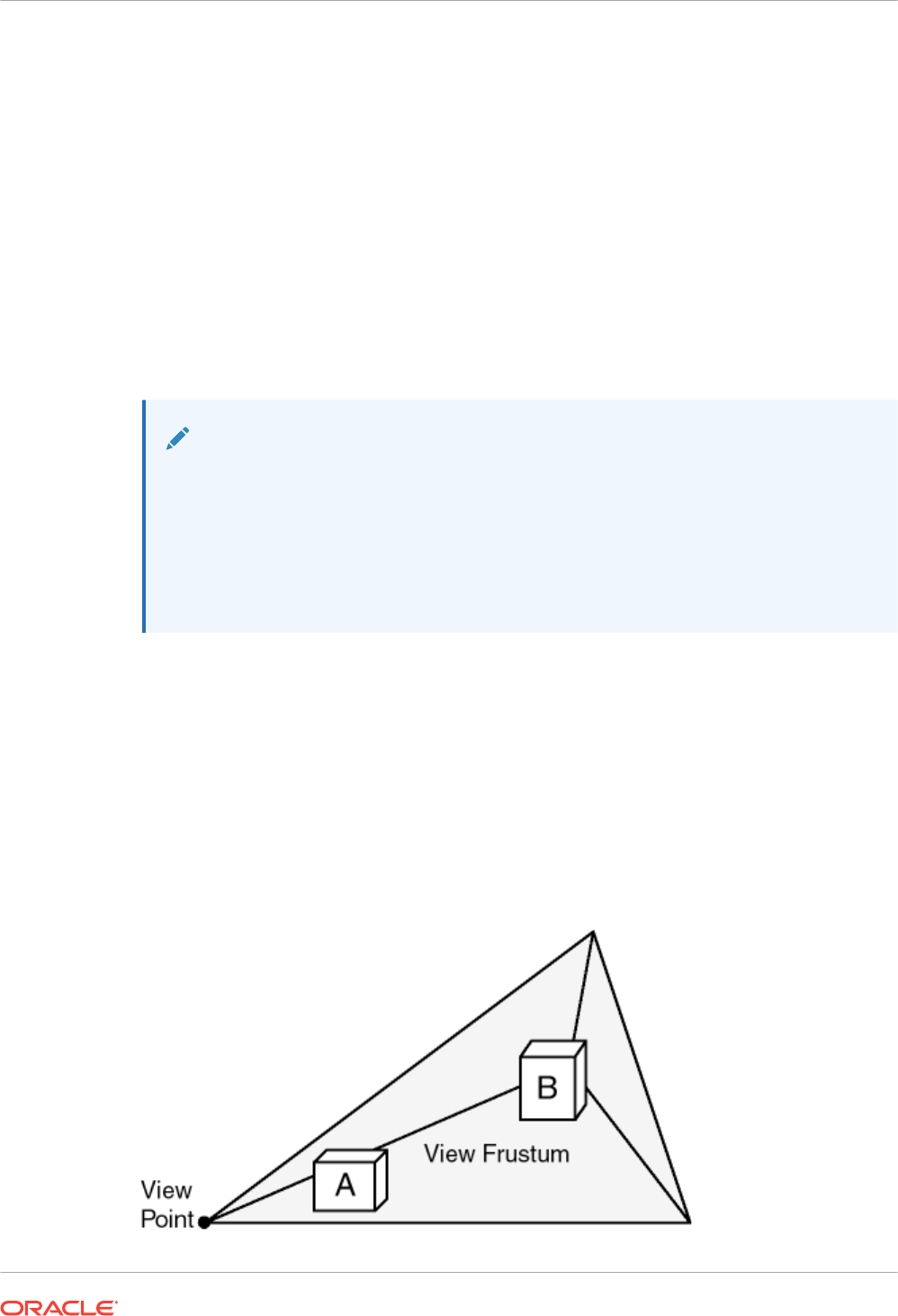
12 cols.column_name,
13 meshes.tin.tin_id;
The example query produces the following output:
Column Name TIN ID Model # Pts Blk Sort Order
---------------- ---------- ---------------------- ----------
--------------------------------
MESHES:TIN 2 TIN 4 TIN by Delaunay
triangulation
MESHES:TIN 3 Mesh 1097 Mesh by
consecutive submesh
2 rows selected.
See Also:
• SDO_TIN_PKG.CREATE_MESHES for more information on how to generate a
3D mesh
• SDO_TIN_PKG.LIST_TIN_COLUMNS to list all the column names containing the
SDO_TIN
object
• SDO_TIN_PKG.LIST_TINS to list all the
SDO_TIN
objects
1.13.2 Modeling Solids
The simplest types of solids can be represented as cuboids, such as a cube or a brick. A more
complex solid is a frustum, which is a pyramid formed by cutting a larger pyramid (with three
or more faces) by a plane parallel to the base of that pyramid. Frustums are sometimes used
as query windows to spatial operators. Frustums and cubes are typically modeled as solid-type
SDO_GEOMETRY objects. Figure 1-9 shows a frustum as a query window, with two spatial
objects at different distances from the view point.
Figure 1-9 Frustum as Query Window for Spatial Objects
Chapter 1
Three-Dimensional Spatial Objects
1-25

Point clouds, which are large collections of points, can sometimes be used to model the
shape or structure of solid and surface geometries. Most applications that use point cloud data
contain queries based on location. Applications can also go outside Spatial to add visibility
logic to perform queries based on both location and visibility.
Most applications that use point cloud data seek to minimize data transfer by retrieving objects
based on their distance from a view point. For example, in Figure 1-9, object B is farther from
the view point than object A, and therefore the application might retrieve object A in great detail
(high resolution) and object B in less detail (low resolution). In most scenarios, the number of
objects or points increases significantly as the distance from the view point increases; and if
farther objects are retrieved at lower resolutions than nearer objects, the number of bytes
returned by the query and the rendering time for the objects decrease significantly.
For storage of point cloud data, you can use either an SDO_PC object or is a flat table. The
approach to use depends on your hardware environment and usage patterns. An advantage of
the flat format is its efficient and dynamic nature, because updates to the point data do not
require reblocking.
The general process for working with a point cloud is as follows, depending on whether the
point cloud data will be stored in an SDO_PC object or in a flat table.
• To use point cloud data stored as an SDO_PC object:
1. Initialize the point cloud, using the SDO_PC_PKG.INIT function.
2. Create the point cloud, using the SDO_PC_PKG.CREATE_PC procedure.
3. As needed for queries, clip the point cloud, using the SDO_PC_PKG.CLIP_PC
function.
4. Additionally, you can use:
– SDO_PC_PKG.TO_GEOMETRY: To convert the result of a clip operation into a
single SDO_GEOMETRY object.
– SDO_PC_PKG.PC_DIFFERENCE: To detect the difference between two point
clouds.
– SDO_PC_PKG.GENERATE_CROSS_SECTION_AS_GEOMS: To perform a cross
section computation of a point cloud.
• To use point cloud data stored in a flat table:
1. Create the table (or a view based on an appropriate table) for the point cloud data.
Each row will contain the values of the first three spatial dimensions of a point, and
optionally values for nonspatial dimensions. The table or view definition must start with
the following columns: VAL_D1 NUMBER, VAL_D2 NUMBER, VAL_D3 NUMBER. It
can also contain columns for point cloud nonspatial dimensions.
2. Populate the table with point data.
3. As needed for queries, clip the point cloud, using the SDO_PC_PKG.CLIP_PC_FLAT
function.
For a Java example of working with point clouds, see the following files:
$ORACLE_HOME/md/demo/PointCloud/examples/java/README.txt
$ORACLE_HOME/md/demo/PointCloud/examples/java/readPointCloud.java
Chapter 1
Three-Dimensional Spatial Objects
1-26

1.13.3 Three-Dimensional Optimized Rectangles
Instead of specifying all the vertices for a three-dimensional rectangle (a polygon in the shape
of rectangle in three-dimensional space), you can represent the rectangle by specifying just the
two corners corresponding to the minimum ordinate values (min-corner) and the maximum
ordinate values (max-corner) for the X, Y, and Z dimensions.
The orientation of a three-dimensional rectangle defined in this way is as follows:
• If the rectangle is specified as <min-corner, max-corner>, the normal points in the positive
direction of the perpendicular third dimension.
• If the rectangle is specified as <max-corner, min-corner>, the normal points in the negative
direction of the perpendicular third dimension.
For example, if the rectangle is in the XY plane and the order of the vertices is <min-corner,
max-corner>, the normal is along the positive Z-axis; but if the order is <max-corner, min-
corner>, the normal is along the negative Z-axis.
Using these orientation rules for rectangles, you can specify the order of the min-corner and
max-corner vertices for a rectangle appropriately so that the following requirements are met:
• The normal for each polygon in a solid always points outward from the solid when the
rectangle is part of the solid.
• An inner rectangle polygon is oriented in the reverse direction as its outer when the
rectangle is part of a surface.
1.13.4 Using Texture Data
Note:
This section describes concepts that you will need to understand for using texture
data with Spatial. However, the texture metadata is not yet fully implemented in
Oracle Spatial, and a viewer is not yet supported. This section will be updated when
texture support is released.
A texture is an image that represents one or more parts of a feature. Textures are commonly
used with visualizer applications (viewers) that display objects stored as spatial geometries.
For example, a viewer might display an office building (three-dimensional solid) using textures,
to allow a more realistic visualization than using just colors. Textures can be used with two-
dimensional and three-dimensional geometries.
In the simplest case, a rectangular geometry can be draped with a texture bitmap. However,
often only a subregion of a texture bitmap is used, as in the following example cases:
• If the texture bitmap contains multiple sides of the same building, as well as the roof and
roof gables. In this case, each bitmap portion is draped over one of the geometry faces.
• If the texture bitmap represents a single panel or window on the building surface, and a
geometric face represents a wall with 15 such panels or windows (five on each of three
floors). In this case, the single texture bitmap is tiled 15 times over the face.
• If the face is non-rectangular sub-faces, such as roof gables. In this case, only a portion
(possible triangular) of the texture bitmap is used.
Chapter 1
Three-Dimensional Spatial Objects
1-27

Figure 1-10 shows a large rectangular surface that, when viewed, appears to consist of three
textures, each of which is repeated multiple times in various places on the surface.
Figure 1-10 Faces and Textures
0 1 2 3 4 5 6 7 8 9 10 11 12 13 14 15
1
2
3
4
5
6
7
8
9
10
11
12
13
14
15
A
C
Texture bitmaps (images):
B
A AB
B
C
C
C
B
B B B
A
A
As shown in
Figure 1-10:
• The entire image is a large surface that consists of 12 smaller rectangular faces (surface
geometries), each of which can be represented by one of three images (labeled A, B, and
C).
• Three texture bitmaps (labeled A, B, and C) can be used to visualize all of the faces. In this
case, bitmap A is used 3 times, bitmap B is used 6 times, and bitmap C is used 3 times.
Figure 1-11 shows a texture bitmap mapped to a triangular face.
Figure 1-11 Texture Mapped to a Face
Texture
bitmap:
Face
geometry:
Texture mapped
to face:
(image) (image)
As shown in Figure 1-11:
Chapter 1
Three-Dimensional Spatial Objects
1-28

• The face (surface geometry) is a triangle. (For example, a side or roof of a building may
contain several occurrences of this face.)
• The texture bitmap (image) is a rectangle, shown in the box in the middle.
• A portion of the texture bitmap represents an image of the face. This portion is shown by a
dashed line in the box on the right.
In your application, you will need to specify coordinates within the texture bitmap to map
the appropriate portion to the face geometry.
To minimize the storage requirements for image data representing surfaces, you should store
images for only the distinct textures that will be needed. The data type for storing a texture is
SDO_ORDINATE_ARRAY, which is used in the SDO_GEOMETRY type definition (explained in
SDO_GEOMETRY Object Type).
For example, assume that the large surface in Figure 1-10 has the following definition:
SDO_GEOMETRY(
2003, -- two-dimensional polygon
NULL,
NULL,
SDO_ELEM_INFO_ARRAY(1,1003,1), -- one polygon (exterior polygon ring)
SDO_ORDINATE_ARRAY(1,1. 1,13, 13,13, 1,13, 1,1)
)
Assume that you have a MY_TEXTURE_COORDINATES table with the following definition:
CREATE TABLE my_texture_coordinates (
texture_coord_id NUMBER PRIMARY KEY,
texture_name VARCHAR2(32),
texture_coordinates SDO_ORDINATE_ARRAY);
Example 1-1 inserts three texture coordinate definitions into this table. For each texture, its
coordinates reflect one of the appropriate smaller rectangles shown in Figure 1-10; however,
you can choose any one of the appropriate rectangles for each texture. In Example 1-1, the
SDO_ORDINATE_ARRAY definitions for each texture reflect a polygon near the top of
Figure 1-10.
Example 1-1 Inserting Texture Coordinate Definitions
INSERT INTO my_texture_coordinates VALUES(
1,
'Texture_A',
SDO_ORDINATE_ARRAY(1,9, 1,5, 5,12, 1,12, 1,9)
);
INSERT INTO my_texture_coordinates VALUES(
2,
'Texture_B',
SDO_ORDINATE_ARRAY(5,9, 9,9, 9,12, 5,12, 5,9)
);
INSERT INTO my_texture_coordinates VALUES(
3,
'Texture_C',
SDO_ORDINATE_ARRAY(1,12, 13,12, 13,13, 1,13, 1,12)
);
• Schema Considerations with Texture Data
Chapter 1
Three-Dimensional Spatial Objects
1-29

1.13.4.1 Schema Considerations with Texture Data
Texture bitmaps (stored as BLOBs or as URLs in VARCHAR2 format) and texture coordinate
arrays (stored using type SDO_ORDINATE_ARRAY) can be stored in the same table as the
SDO_GEOMETRY column or in separate tables; however, especially for the texture bitmaps, it
is usually better to use separate tables. Texture bitmaps are likely to be able to be shared
among features (such as different office buildings), but texture coordinate definitions are less
likely to be sharable among features. (For example, many office buildings may share the same
general type of glass exterior, but few of the buildings have the same number of windows and
floors. In designing your textures and applications, you must consider how many buildings use
the same texture subregion or drape the texture in the same size of repetitive matrix.)
An exception is a texture coordinate array that drapes an entire texture bitmap over a
rectangular geometric face. In this case, the texture coordinate array can be specified as (0,0,
1,0, 1,1, 0,1, 1,1), defined by vertices "lower left", "lower right", "upper right", "upper left", and
closing with "lower left". Many data sets use this texture coordinate array extensively, because
they have primarily rectangular faces and they store one facade for each texture bitmap.
If you used separate tables, you could link them to the surface geometries using foreign keys,
as in Example 1-2.
Example 1-2 Creating Tables for Texture Coordinates, Textures, and Surfaces
-- One row for each texture coordinates definition.
CREATE TABLE my_texture_coordinates (
texture_coord_id NUMBER PRIMARY KEY,
texture_coordinates SDO_ORDINATE_ARRAY);
-- One row for each texture.
CREATE TABLE my_textures(
texture_id NUMBER PRIMARY KEY,
texture BLOB);
-- One row for each surface (each individual "piece" of a
-- potentially larger surface).
CREATE TABLE my_surfaces(
surface_id NUMBER PRIMARY KEY,
surface_geometry SDO_GEOMETRY,
texture_id NUMBER,
texture_coord_id NUMBER,
CONSTRAINT texture_id_fk
FOREIGN KEY (texture_id) REFERENCES my_textures(texture_id),
CONSTRAINT texture_coord_id_fk
FOREIGN KEY (texture_coord_id) REFERENCES
my_texture_coordinates(texture_coord_id));
1.13.5 Validation Checks for Three-Dimensional Geometries
The SDO_GEOM.VALIDATE_GEOMETRY_WITH_CONTEXT and
SDO_GEOM.VALIDATE_LAYER_WITH_CONTEXT subprograms can validate two-
dimensional and three-dimensional geometries. For a three-dimensional geometry, these
subprograms perform any necessary checks on any two-dimensional geometries (see the
Usage Notes for SDO_GEOM.VALIDATE_GEOMETRY_WITH_CONTEXT) within the overall
three-dimensional geometry, but also several checks specific to the three-dimensional nature
of the overall object.
For a simple solid (one outer surface and any number of inner surfaces), these subprograms
perform the following checks:
Chapter 1
Three-Dimensional Spatial Objects
1-30

• Closedness: The solid must be closed.
• Reachability: Each face of a solid must have a full-edge intersection with its neighboring
faces, and all faces must be reachable from any face. (However, inner shells are ignored,
because inner shells can, by definition, be not connected to the other shells.)
• Inner-outer disjointedness: An inner surface must not intersect the outer surface at more
than a point or a line; that is, there must be no overlapping areas with inner surfaces.
• No surface patch: No additional surfaces can be defined on the surfaces that make up the
solid.
• Orientation: For all surfaces, the vertices must be aligned so that the normal vector (or
surface normal, or "the normal") points to the outside of (away from) the outer solid. Thus,
the volume of the outer solid must be greater than zero, and the volume of any inner solid
must be less than zero.
For a composite solid (one or more solids connected to each other), these subprograms
perform the following checks:
• Connectedness: All solids of a composite solid must share at least one face.
• Zero-volume intersections: Any intersections of the solids in a composite solid must have a
volume of zero.
For a multisolid (one or more solids, each of which is a simple or composite solid), these
subprograms perform the following check:
• Disjointedness: Any two solids of a multisolid can share points or lines, but must not
intersect in any other manner.
1.14 Geocoding
Geocoding is the process of converting tables of address data into standardized address,
location, and possibly other data.
The result of a geocoding operation includes the pair of longitude and latitude coordinates that
correspond with the input address or location. For example, if the input address is 22
Monument Square, Concord, MA 01742, the longitude and latitude coordinates in the result of
the geocoding operation may be (depending on the geocoding data provider) -71.34937 and
42.46101, respectively.
Given a geocoded address, you can perform proximity or location queries using a spatial
engine, such as Oracle Spatial, or demographic analysis using tools and data from Oracle's
business partners. In addition, you can use geocoded data with other spatial data such as
block group, postal code, and county code for association with demographic information.
Results of analyses or queries can be presented as maps, in addition to tabular formats, using
third-party software integrated with Oracle Spatial.
For conceptual and usage information about the geocoding capabilities of Oracle Spatial, see
Geocoding Address Data. For reference information about the MDSYS.SDO_GCDR PL/SQL
package, see SDO_GCDR Package (Geocoding) .
1.15 Location Data Enrichment
Oracle Spatial includes a place name data set, with hierarchical geographical data from HERE,
that you can load into the database.
Chapter 1
Geocoding
1-31

You can then then search this place name data set using the SDO_UTIL.GEO_SEARCH
function. The data set includes commonly used textual location data such as place names,
addresses and partial addresses, and latitude and longitude information.
Location tags are extracted from text data, and are matched with well known place names
using Oracle Text and enhanced with other geographic information associated with the well
known place names.
The results can be stored as additional attributes with the original data.
This feature enables you to process less structured geographic and location data so that the
information can be categorized, compared, filtered, and associated with other data. For
example, data with only partial names can be enriched to include city, county, state, and
country, allowing it to be joined or analyzed with other data sets that may have state level
information. This is especially useful when comparing Big Data results with structured
information in operational systems and data warehouses.
Setting Up and Using Location Data Enrichment Support
To use the location data enrichment support, you just perform certain setup actions, such as
editing scripts that will create the necessary database objects and load the data set into Oracle
Database, and running those scripts.
1. Go to
$ORACLE_HOME//md/demo/GeoSearch
, which contains all the required files.
2. Read the
README
file, a text file containing an overview of the basic steps.
3. Perform the actions indicated in the
README
file.
These actions include reading the
LICENSES.TXT
file, creating a single zip file from split
files, editing the
load_data.sql
and
create_index.sql
script files (which contain
explanatory comments), and running those scripts.
The
create_index.sql
file includes some example queries using the
SDO_UTIL.GEO_SEARCH function. You can use those examples, plus the
SDO_UTIL.GEO_SEARCH reference and usage information, to develop your own uses of the
location data enrichment support.
• ELOC_ADMIN_AREA_SEARCH Table
• Adding User Data to the Geographic Name Hierarchy
1.15.1 ELOC_ADMIN_AREA_SEARCH Table
The ELOC_ADMIN_AREA_SEARCH table is used to store the data for location data
enrichment. It is created only if you have performed the required setup actions described in
Location Data Enrichment, and it is created in the database schema that you chose.
This table is accessed by the SDO_UTIL.GEO_SEARCH procedure. The table has the
following columns.
Table 1-3 LOC_ADMIN_AREA_SEARCH Table
Column Name Description
AREA_ID Unique ID for the place name.
Chapter 1
Location Data Enrichment
1-32

Table 1-3 (Cont.) LOC_ADMIN_AREA_SEARCH Table
Column Name Description
FULL_NAME The name of the place as a searchable string. For example,
“NASHUA,HILLSBOROUGH,NEW HAMPSHIRE,NH,UNITED STATES,USA” is the
searchable name for the city of Nashua in NH, USA.
This entry is a concatenated list of all possible names for each level of the name
hierarchy. That is, for state it can have both the abbreviation and the full name.
Similarly, for country it can have both the abbreviation and the full name. This
enables the search to find this entry even when different search terms are used for
each of these administrative areas.
AREA_NAME The actual area name of the administrative place.
KEY A standardized text key that is returned from the search API. This is a normalized
standard key that can be used for joining the search term with other terms.
LANG_CODE 3- letter ISO code of the language used for this entry.
PART_ID A number that is used when this table is partitioned (see the README for more
details).
CENTER_LONG Longitude of the place name.
CENTER_LAT Latitude of the place name.
POPULATION A number that is used to order the results when multiple matches are found for a
given search term. The intent is to return more populated areas first before retuning
less populated areas where multiple matches are found for the same search term.
1.15.2 Adding User Data to the Geographic Name Hierarchy
In some cases, users might want to add their own data to augment the data provided by
Oracle. For example, if the users wants to create an entry for a park in the city (like Central
Park in New York City) they can create an entry for it in this table.
For example, they can do :
insert into ELOC_ADMIN_AREA_SEARCH values (1469286010, 'CENTRAL PARK,NEW YORK
CITY,NEW YORK,NYC,RICHMOND,NEW YORK,NY,UNITED STATES,USA', 'CENTRAL PARK',
'CENTRAL PARK|NEW YORK|RICHMOND|NEW YORK|UNITED STATES', 'ENG', 7,
73.9654,40.7829, 0);
commit;
The COMMIT statement after inserting new data is important, because the text index performs
a synchronization only after the commit is issued.
In this example, the area_id is chosen to be some value that does not already exist in the
table, and a random partition_id value is used (7 in this case). However, a suitable value
should be chosen based on the partitioning scheme used for the table (see the README for
more details).
Now a search for central park will result a match:
select * from table(sdo_util.geo_search('central park,new york,NY,UNITED
STATES'));
CENTRAL PARK
CENTRAL PARK|NEW YORK|RICHMOND|NEW YORK|UNITED STATES
ENG 73.9654 40.7829 100
Chapter 1
Location Data Enrichment
1-33

1.16 JSON and GeoJSON Support in Oracle Spatial
Spatial supports the use of JSON and GeoJSON objects to store, index, and manage
geographic data that is in JSON (JavaScript Object Notation) format.
JSON support, introduced in Release 18.1, substantially expands the limited GeoJSON
support available in the previous release, in that it supports a larger range of geometries,
including 2D and 3D, solid, surface, and LRS geometries. While the Spatial GeoJSON-specific
APIs are still supported, you are encouraged to use the more comprehensive JSON support.
• JSON Support in Oracle Spatial
Spatial supports the use of JSON objects to store, index, and manage geographic data
that is in JSON (JavaScript Object Notation) format.
• GeoJSON Support in Oracle Spatial
Oracle Spatial supports the use of GeoJSON objects to store, index, and manage
geographic data that is in JSON (JavaScript Object Notation) format.
• JSON Schema for Spatial Geometry Objects
Spatial uses an internal schema for storing spatial data in JSON (JavaScript Object
Notation) format.
1.16.1 JSON Support in Oracle Spatial
Spatial supports the use of JSON objects to store, index, and manage geographic data that is
in JSON (JavaScript Object Notation) format.
You can convert any Oracle Spatial SDO_GEOMETRY object to a JSON geometry object, and
geometry JSON object back to an SDO_GEOMETRY object.
JSON support in Spatial includes the following:
• SDO_UTIL.TO_JSON converts an SDO_GEOMETRY object to a JSON object in CLOB
format.
• SDO_UTIL.TO_JSON_VARCHAR converts an SDO_GEOMETRY object to a JSON object
in VARCHAR2 format.
• SDO_UTIL.FROM_JSON converts a JSON object (in CLOB or VARCHAR2 format) to an
SDO_GEOMETRY object. This function can also convert a GeoJSON object to an
SDO_GEOMETRY object.
Example 1-3 JSON Support in Spatial
This example shows some operations using the JSON support in Oracle Spatial. The example
creates a simple table with a JSON column and an SDO_GEOMETRY column, inserts some
sample data, performs some simple queries, creates a spatial index, and performs a query
using the SDO_WITHIN_DISTANCE operator.
The example uses the following JSON-related feature of Oracle Database, which is
documented in Oracle Database JSON Developer's Guide:
• The IS JSON Oracle SQL condition in a check constraint in the CREATE TABLE statement
to ensure that a column contains JSON data
Chapter 1
JSON and GeoJSON Support in Oracle Spatial
1-34

The example includes descriptive comments and the output of the SQL statements. (The
output has been reformatted for readability.)
-- Some operations using JSON support in Spatial.
-- Create a table with 3 columns: one JSONC (JSON CLOB), one JSONV (JSON
VARCHAR2),
-- and one SDO_GEOMETRY.
CREATE TABLE JSON_TBL (
jsonc CLOB, jsonv VARCHAR2(4000),
geom SDO_GEOMETRY,
CONSTRAINT json_tbl_json CHECK (jsonc IS JSON) );
Table created.
-- Test the constraint
INSERT INTO json_tbl VALUES ('Not JSON', NULL, NULL);
ORA-02290: check constraint (SCOTT.JSON_TBL_JSON) violated
-- Insert some data (2 points).
INSERT INTO JSON_TBL(jsonc)
VALUES ('{"srid": 8307, "point": {"directposition": [123.4, -10.1]}}');
1 row created.
INSERT INTO JSON_TBL(jsonc)
VALUES ('{"srid": 8307, "point": {"directposition": [123.5, -10.2]}}');
1 row created.
COMMIT;
Commit complete.
-- Update the table with the VARCHAR formatted JSON object and
-- an SDO_GEOMETRY created from a JSON object
UPDATE JSON_TBL SET
jsonv=SDO_UTIL.TO_JSON_VARCHAR(SDO_UTIL.FROM_JSON(jsonc)),
geom=SDO_UTIL.FROM_JSON(jsonc);
2 rows updated.
COMMIT;
SELECT jsonc, jsonv, geom FROM json_tbl;
JSONC
-------
JSONV
-------
GEOM(SDO_GTYPE, SDO_SRID, SDO_POINT(X, Y, Z), SDO_ELEM_INFO, SDO_ORDINATES)
-----------------------------------------------------------------------
{"srid": 8307, "point": {"directposition": [123.4, -10.1]}}
{"srid": 8307, "point": {"directposition": [123.4, -10.1]}}
SDO_GEOMETRY(2001, 8307, SDO_POINT_TYPE(123.4, -10.1, NULL), NULL, NULL)
{"srid": 8307, "point": {"directposition": [123.5, -10.2]}}
{"srid": 8307, "point": {"directposition": [123.5, -10.2]}}
SDO_GEOMETRY(2001, 8307, SDO_POINT_TYPE(123.5, -10.2, NULL), NULL, NULL)
Chapter 1
JSON and GeoJSON Support in Oracle Spatial
1-35

1.16.2 GeoJSON Support in Oracle Spatial
Oracle Spatial supports the use of GeoJSON objects to store, index, and manage geographic
data that is in JSON (JavaScript Object Notation) format.
You can convert Spatial SDO_GEOMETRY objects to GeoJSON objects, and GeoJSON
objects to SDO_GEOMETRY objects. You can use spatial operators, functions, and a special
SDO_GEOMETRY method to work with GeoJSON data.
GeoJSON support in Spatial includes the following:
• SDO_UTIL.TO_GEOJSON function to convert an SDO_GEOMETRY object to a GeoJSON
object..
• SDO_UTIL.FROM_GEOJSON function to convert a GeoJSON object to an
SDO_GEOMETRY object.
• Get_GeoJson method (member function) of the SDO_GEOMETRY type (see
SDO_GEOMETRY Methods for an explanation and an example).
Example 1-4 GeoJSON Support in Spatial
This example shows some operations using the GeoJSON support in Spatial. The example
creates a simple table with a GeoJSON column and an SDO_GEOMETRY column, inserts
some sample data, performs some simple queries, creates a spatial index, and performs a
query using the SDO_WITHIN_DISTANCE operator.
The example uses the following JSON-related features of Oracle Database, which are
documented in Oracle Database JSON Developer's Guide:
• The JSON_VALUE Oracle SQL function with
RETURNING SDO_GEOMETRY
to return
SDO_GEOMETRY objects reflecting GeoJSON objects
• The IS JSON Oracle SQL condition in a check constraint in the CREATE TABLE statement
to ensure that a column contains JSON data
The example includes descriptive comments and the output of the SQL statements. (The
output has been reformatted for readability.)
-- Some operations using GeoJSON support in Spatial.
-- Create a table with 2 columns: one GeoJSON, one SDO_GEOMETRY.
CREATE TABLE GEO_TABLE (geojson_col VARCHAR2(4000), geom_col SDO_GEOMETRY,
CONSTRAINT CHECK (geojson_col IS JSON));
Table created.
-- Insert some data (2 points).
INSERT INTO GEO_TABLE(geojson_col)
values ('{"a":{"type":"Point","coordinates":[+123.4,+10.1]}}');
1 row created.
INSERT INTO GEO_TABLE(geojson_col)
values ('{"a":{"type":"Point","coordinates":[+123.5,-10.1]}}');
1 row created.
commit;
Chapter 1
JSON and GeoJSON Support in Oracle Spatial
1-36

Commit complete.
SQL> -- For each geojson_col value, return what its SDO_GEOMETRY equivalent
would be.
SQL> SELECT JSON_VALUE(geojson_col, '$.a' RETURNING SDO_GEOMETRY) from
GEO_TABLE;
JSON_VALUE(GEOJSON_COL,'$.A'RETURNINGSDO_GEOMETRY)(SDO_GTYPE, SDO_SRID,
SDO_POIN
------------------------------------------------------------------------------
--
SDO_GEOMETRY(2001, 4326, SDO_POINT_TYPE(123.4, 10.1, NULL), NULL,
NULL)
SDO_GEOMETRY(2001, 4326, SDO_POINT_TYPE(123.5, -10.1, NULL), NULL,
NULL)
-- For a specified GeoJSON object definition, return what its SDO_GEOMETRY
-- equivalent would be.
SELECT JSON_VALUE('{"type":"Point","coordinates":[+123.5,-10.1]}',
'$' RETURNING SDO_GEOMETRY) from DUAL;
JSON_VALUE('{"TYPE":"POINT","COORDINATES":
[+123.5,-10.1]}','$'RETURNINGSDO_GEOME
------------------------------------------------------------------------------
--
SDO_GEOMETRY(2001, 4326, SDO_POINT_TYPE(123.5, -10.1, NULL), NULL,
NULL)
-- Update to populate geom_col with SDO_GEOMETRY objects reflecting the JSON
data
-- in the geojson_col column.
UPDATE GEO_TABLE
set geom_col = JSON_VALUE(geojson_col, '$.a' RETURNING SDO_GEOMETRY);
2 rows updated.
commit;
Commit complete.
-- Create spatial index on the returned SDO_GEOMETRY objects from the JSON
data.
CREATE INDEX GEO_TABLE_IX
ON GEO_TABLE
(
JSON_VALUE(geojson_col, '$.a' RETURNING SDO_GEOMETRY)
)
INDEXTYPE IS MDSYS.SPATIAL_INDEX_V2;
Index created.
-- SDO_WITHIN_DISTANCE query: Are two grometries within 100 miles apart?
SELECT 1
FROM GEO_TABLE
WHERE SDO_WITHIN_DISTANCE(
JSON_VALUE(geojson_col, '$.a' RETURNING SDO_GEOMETRY),
Chapter 1
JSON and GeoJSON Support in Oracle Spatial
1-37

JSON_VALUE('{"type":"Point","coordinates":[+123.5,-10.1]}',
'$' RETURNING SDO_GEOMETRY),
'distance=100 unit=mile') = 'TRUE';
1
----------
1
1.16.3 JSON Schema for Spatial Geometry Objects
Spatial uses an internal schema for storing spatial data in JSON (JavaScript Object Notation)
format.
The information if this topic is useful if you want to write a parser to read such data on the
client side. The JSON schema used for spatial data is as follows.
"$schema": "http://json-schema.org/draft-06/schema#",
"type": "object",
"anyOf": [
{ "$ref": "#/definitions/CompoundCurveSchema" },
{ "$ref": "#/definitions/CurveSchema" },
{ "$ref": "#/definitions/MultiGeometrySchema" },
{ "$ref": "#/definitions/PointSchema" },
{ "$ref": "#/definitions/PolygonSchema" },
{ "$ref": "#/definitions/SolidSchema" },
{ "$ref": "#/definitions/SurfaceSchema" }
],
"definitions": {
"CompoundCurveSchema": {
"description": "A JSON schema for compound curve geometry",
"type": "object",
"properties": {
"srid": { "$ref": "#/definitions/srid" },
"spatialdimension": { "$ref": "#/definitions/spatialdimension" },
"compoundcurve": { "$ref": "#/definitions/compoundcurve" }
}
},
"CurveSchema": {
"description": "A JSON schema for curve geometry",
"type": "object",
"oneOf": [{
"required": [ "circulararc" ],
"properties": {
"srid": { "$ref": "#/definitions/srid" },
"spatialdimension": { "$ref": "#/definitions/spatialdimension" },
"circulararc": { "$ref": "#/definitions/circulararc" }
}
}, {
"required": [ "line " ],
"properties": {
"srid": { "$ref": "#/definitions/srid" },
"spatialdimension": { "$ref": "#/definitions/spatialdimension" },
"line": { "$ref": "#/definitions/line" }
Chapter 1
JSON and GeoJSON Support in Oracle Spatial
1-38

}
}, {
"required": [ "nurbscurve " ],
"properties": {
"srid": { "$ref": "#/definitions/srid" },
"spatialdimension": { "$ref": "#/definitions/spatialdimension" },
"nurbscurve": { "$ref": "#/definitions/nurbscurve" }
}}]
},
"MultiGeometrySchema": {
"description": "JSON schema for collections & multi-* curves, points
and polygons",
"type": "object",
"properties": {
"srid": { "$ref": "#/definitions/srid" },
"spatialdimension": { "$ref": "#/definitions/spatialdimension" },
"geometrycollection": { "$ref": "#/definitions/geometrycollection" }
}
},
"PointSchema": {
"description": "A JSON schema for point geometry",
"type": "object",
"properties": {
"srid": { "$ref": "#/definitions/srid" },
"spatialdimension": { "$ref": "#/definitions/spatialdimension" },
"point": { "$ref": "#/definitions/point" }
}
},
"PolygonSchema": {
"description": "A JSON schema for polygon geometry",
"type": "object",
"properties": {
"srid": { "$ref": "#/definitions/srid" },
"spatialdimension": { "$ref": "#/definitions/spatialdimension" },
"polygon": { "$ref": "#/definitions/polygon" }
}
},
"SolidSchema": {
"description": "A JSON schema for surface geometry",
"type": "object",
"properties": {
"srid": { "$ref": "#/definitions/srid" },
"spatialdimension": { "$ref": "#/definitions/spatialdimension" },
"polygon": { "$ref": "#/definitions/solid" }
}
},
"SurfaceSchema": {
"description": "A JSON schema for surface geometry",
"type": "object",
"properties": {
"srid": { "$ref": "#/definitions/srid" },
"spatialdimension": { "$ref": "#/definitions/spatialdimension" },
"polygon": { "$ref": "#/definitions/polygons" }
}
},
Chapter 1
JSON and GeoJSON Support in Oracle Spatial
1-39

"circle": {
"description": "An SDO_GEOMETRY optimized circle Polygon",
"type": "object",
"required": [ "datapoints" ],
"properties": {
"datapoints": { "$ref": "#/definitions/datapoints" }
}
},
"circulararc": {
"description": "An SDO_GEOMETRY arc string",
"type": "object",
"required": [ "datapoints" ],
"properties": {
"datapoints": { "$ref": "#/definitions/datapoints" }
}
},
"geometrycollection": {
"description": "A collection of SDO_GEOMETRY",
"type": "object",
"required": [ "geometries" ],
"properties": {
"geometries": { "$ref": "#/definitions/geometries" }
}
},
"knot": {
"description": "A Knot (value/multiplicity pair) in a NURBS curve",
"type": "object",
"required": [ "value", "multiplicity" ],
"properties": {
"value": { "$ref": "#/definitions/value" },
"multiplicity": { "$ref": "#/definitions/multiplicity" }
}
},
"line": {
"description": "An SDO_GEOMETRY linestring",
"type": "object",
"required": [ "datapoints" ],
"properties": {
"datapoints": { "$ref": "#/definitions/datapoints" }
}
},
"multipoint": {
"description": "An SDO_GEOMETRY MultiPoint",
"type": "object",
"required": [ "datapoints" ],
"properties": {
"datapoints": { "$ref": "#/definitions/datapoints" }
}
},
"nurbscurve": {
"description": "An SDO_GEOMETRY nurbscurve",
"type": "object",
"required": [ "degree", "controlpoints", "knots" ],
"properties": {
"degree": { "type": "integer" },
"controlpoints": { "$ref": "#/definitions/controlpoints" },
Chapter 1
JSON and GeoJSON Support in Oracle Spatial
1-40

"knots": { "$ref": "#/definitions/knots" }
}
},
"nurbspoint": {
"description": "A weighted point/weight pair in a NURBS curve",
"type": "object",
"required": [ "weightedpoint", "weight" ],
"properties": {
"weightedpoint": { "$ref": "#/definitions/weightedpoint" },
"weight": { "$ref": "#/definitions/weight" }
}
},
"point": {
"description": "An SDO_GEOMETRY Point",
"type": "object",
"required": [ "directposition" ],
"properties": {
"optimized": { "$ref": "#/definitions/optimized" },
"directposition": { "$ref": "#/definitions/directposition" }
}
},
"polygon": {
"description": "An SDO_GEOMETRY Polygon",
"type": "object",
"required": [ "boundary" ],
"properties": {
"boundary": { "$ref": "#/definitions/boundary" }
}
},
"rectangle": {
"description": "An SDO_GEOMETRY optimized rectangle Polygon",
"type": "object",
"required": [ "datapoints" ],
"properties": {
"datapoints": { "$ref": "#/definitions/datapoints" }
}
},
"solid": {
"description": "An SDO_GEOMETRY solid",
"type": "object",
"required": [ "surfaces" ],
"properties": {
"datapoints": { "$ref": "#/definitions/surfaces" }
}
},
"surface": {
"description": "An SDO_GEOMETRY surface",
"type": "object",
"required": [ "polygons" ],
"properties": {
"datapoints": { "$ref": "#/definitions/polygons" }
}
},
"boundary": {
"description": "An array of geometries that make up a polygon's
Chapter 1
JSON and GeoJSON Support in Oracle Spatial
1-41

boundary",
"type": "array",
"minItems": 1,
"items":{
"anyOf": [
{ "$ref": "#/definitions/circle" },
{ "$ref": "#/definitions/circulararc" },
{ "$ref": "#/definitions/compoundcurve" },
{ "$ref": "#/definitions/line" },
{ "$ref": "#/definitions/rectangle" }
]
}
},
"compoundcurve": {
"description": "An array of curves the make up the compound curve",
"type": "array",
"minItems": 2,
"items":{
"anyOf": [
{ "$ref": "#/definitions/circulararc" },
{ "$ref": "#/definitions/line" },
{ "$ref": "#/definitions/nurbscurve" }
]
}
},
"controlpoints": {
"description": "An array of nurbspoints in a NURBS curve",
"type": "array",
"minItems": 1,
"items": { "$ref": "#/definitions/nurbspoint" }
},
"datapoints": {
"description": "An array of coordinates",
"type": "array",
"minItems": 4,
"items": { "type": "number" }
},
"directposition": {
"description": "A single coordinate",
"type": "array",
"minItems": 2,
"maxItems": 3,
"items": { "type": "number" }
},
"geometries": {
"description": "An array of geometries",
"type": "array",
"minItems": 1,
"items":{
"anyOf": [
{ "$ref": "#/definitions/circulararc" },
{ "$ref": "#/definitions/line" },
{ "$ref": "#/definitions/nurbscurve" },
{ "$ref": "#/definitions/point" },
{ "$ref": "#/definitions/polygon" },
{ "$ref": "#/definitions/multipoint" }
Chapter 1
JSON and GeoJSON Support in Oracle Spatial
1-42

]
}
},
"knots": {
"description": "An array of Knots in a NURBS curve",
"type": "array",
"minItems": 1,
"items": { "$ref": "#/definitions/knot" }
},
"multiplicity": {
"description": "A Multiplicity in a NURBS curve",
"type": "integer",
"minimum": 1
},
"optimized": {
"description": "An SDO optimized point",
"type": "boolean",
"default": true
},
"polygons": {
"description": "An array of polygon geometries that make up a surface",
"type": "array",
"minItems": 1,
"items": { "$ref": "#/definitions/polygon" }
},
"spatialdimension": {
"description": "A geometry's spatial dimension ",
"minimum": 2,
"maximum": 3,
"type": "integer"
},
"srid": {
"description": "A geometry's SRID",
"type": "integer"
},
"surfaces": {
"description": "An array of surface geometries that make up a solid",
"type": "array",
"minItems": 1,
"items": { "$ref": "#/definitions/surface" }
},
"value": {
"description": "A Value in a NURBS curve",
"type": "number"
},
"weight": {
"description": "Weight of a weighted point in a NURBS curve",
"type": "integer"
},
"weightedpoint": {
"description": "An array of weighted points in a NURBS curve",
"type": "array",
"minItems": 2,
"maxItems": 2,
"items": { "type": "number" }
}
Chapter 1
JSON and GeoJSON Support in Oracle Spatial
1-43

}
}
Example 1-5 JSON Representations of Various Spatial Geometries
The following examples show JSON representations produced by Spatial for various types of
spatial geometries.
Point: JGeometry (gtype=1, dim=2, srid=0, Point=(10.0,5.0))
{
"point" : {
"directposition" : [ 10.0, 5.0 ]
}
}
Line segment: JGeometry (gtype=2, dim=2, srid=0,
ElemInfo(1,2,1),
Ordinates(10.0,10.0
20.0,10.0
))
{
"line" : {
"datapoints" : [ [ 10.0, 10.0 ], [ 20.0, 10.0 ] ]
}
}
Arc segment: JGeometry (gtype=2, dim=2, srid=0,
ElemInfo(1,2,2),
Ordinates(10.0,15.0
15.0,20.0
20.0,15.0
))
{
"circulararc" : {
"datapoints" : [ [ 10.0, 15.0 ], [ 15.0, 20.0 ], [ 20.0, 15.0 ] ]
},
"interpolation" : "CIRCULAR"
}
Line string: JGeometry (gtype=2, dim=2, srid=0,
ElemInfo(1,2,1),
Ordinates(10.0,25.0
20.0,30.0
25.0,25.0
30.0,30.0
))
{
"line" : {
"datapoints" : [ [ 10.0, 25.0 ], [ 20.0, 30.0 ], [ 25.0, 25.0 ], [ 30.0,
30.0 ] ]
}
}
Arc string: JGeometry (gtype=2, dim=2, srid=0,
ElemInfo(1,2,2),
Ordinates(10.0,35.0
15.0,40.0
20.0,35.0
25.0,30.0
30.0,35.0
Chapter 1
JSON and GeoJSON Support in Oracle Spatial
1-44

))
{
"circulararc" : {
"datapoints" : [ [ 10.0, 35.0 ], [ 15.0, 40.0 ], [ 20.0, 35.0 ], [ 25.0,
30.0 ], [ 30.0, 35.0 ] ]
},
"interpolation" : "CIRCULAR"
}
Compound line string: JGeometry (gtype=2, dim=2, srid=0,
ElemInfo(1,4,3,1,2,1,3,2,2,7,2,1),
Ordinates(10.0,45.0
20.0,45.0
23.0,48.0
20.0,51.0
10.0,51.0
))
{
"compoundcurve" : [ {
"line" : {
"datapoints" : [ [ 10.0, 45.0 ], [ 20.0, 45.0 ] ]
}
}, {
"circulararc" : {
"datapoints" : [ [ 20.0, 45.0 ], [ 23.0, 48.0 ], [ 20.0, 51.0 ] ]
},
"interpolation" : "CIRCULAR"
}, {
"line" : {
"datapoints" : [ [ 20.0, 51.0 ], [ 10.0, 51.0 ] ]
}
} ]
}
Closed line string: JGeometry (gtype=2, dim=2, srid=0,
ElemInfo(1,2,1),
Ordinates(10.0,55.0
15.0,55.0
20.0,60.0
10.0,60.0
10.0,55.0
))
{
"line" : {
"datapoints" : [ [ 10.0, 55.0 ], [ 15.0, 55.0 ], [ 20.0, 60.0 ], [ 10.0,
60.0 ], [ 10.0, 55.0 ] ]
}
}
Closed arc string: JGeometry (gtype=2, dim=2, srid=0,
ElemInfo(1,2,2),
Ordinates(15.0,65.0
10.0,68.0
15.0,70.0
20.0,68.0
15.0,65.0
))
{
"circulararc" : {
Chapter 1
JSON and GeoJSON Support in Oracle Spatial
1-45

"datapoints" : [ [ 15.0, 65.0 ], [ 10.0, 68.0 ], [ 15.0, 70.0 ], [ 20.0,
68.0 ], [ 15.0, 65.0 ] ]
},
"interpolation" : "CIRCULAR"
}
Closed mixed line: JGeometry (gtype=2, dim=2, srid=0,
ElemInfo(1,4,2,1,2,1,7,2,2),
Ordinates(10.0,78.0
10.0,75.0
20.0,75.0
20.0,78.0
15.0,80.0
10.0,78.0
))
{
"compoundcurve" : [ {
"line" : {
"datapoints" : [ [ 10.0, 78.0 ], [ 10.0, 75.0 ], [ 20.0, 75.0 ],
[ 20.0, 78.0 ] ]
}
}, {
"circulararc" : {
"datapoints" : [ [ 20.0, 78.0 ], [ 15.0, 80.0 ], [ 10.0, 78.0 ] ]
},
"interpolation" : "CIRCULAR"
} ]
}
Self-crossing line: JGeometry (gtype=2, dim=2, srid=0,
ElemInfo(1,2,1),
Ordinates(10.0,-75.0
20.0,-70.0
20.0,-75.0
10.0,-70.0
10.0,-75.0
))
{
"line" : {
"datapoints" : [ [ 10.0, -75.0 ], [ 20.0, -70.0 ], [ 20.0, -75.0 ],
[ 10.0, -70.0 ], [ 10.0, -75.0 ] ]
}
}
Polygon: JGeometry (gtype=3, dim=2, srid=0,
ElemInfo(1,1003,1),
Ordinates(10.0,-55.0
15.0,-55.0
20.0,-50.0
10.0,-50.0
10.0,-55.0
))
{
"polygon" : {
"boundary" : [ {
"line" : {
"datapoints" : [ [ 10.0, -55.0 ], [ 15.0, -55.0 ], [ 20.0, -50.0 ],
[ 10.0, -50.0 ], [ 10.0, -55.0 ] ]
}
Chapter 1
JSON and GeoJSON Support in Oracle Spatial
1-46

} ]
}
}
Arc polygon: JGeometry (gtype=3, dim=2, srid=0,
ElemInfo(1,1003,2),
Ordinates(15.0,-45.0
20.0,-42.0
15.0,-40.0
10.0,-42.0
15.0,-45.0
))
{
"polygon" : {
"boundary" : [ {
"circulararc" : {
"datapoints" : [ [ 15.0, -45.0 ], [ 20.0, -42.0 ], [ 15.0, -40.0 ],
[ 10.0, -42.0 ], [ 15.0, -45.0 ] ]
},
"interpolation" : "CIRCULAR"
} ]
}
}
Compound polygon: JGeometry (gtype=3, dim=2, srid=0,
ElemInfo(1,1005,2,1,2,1,7,2,2),
Ordinates(10.0,-32.0
10.0,-35.0
20.0,-35.0
20.0,-32.0
15.0,-30.0
10.0,-32.0
))
{
"polygon" : {
"boundary" : [ {
"compoundcurve" : [ {
"line" : {
"datapoints" : [ [ 10.0, -32.0 ], [ 10.0, -35.0 ], [ 20.0, -35.0 ],
[ 20.0, -32.0 ] ]
}
}, {
"circulararc" : {
"datapoints" : [ [ 20.0, -32.0 ], [ 15.0, -30.0 ], [ 10.0, -32.0 ] ]
},
"interpolation" : "CIRCULAR"
} ]
} ]
}
}
Rectangle: JGeometry (gtype=3, dim=2, srid=0,
ElemInfo(1,1003,1),
Ordinates(10.0,-25.0
20.0,-25.0
20.0,-20.0
10.0,-20.0
10.0,-25.0
))
Chapter 1
JSON and GeoJSON Support in Oracle Spatial
1-47

{
"polygon" : {
"boundary" : [ {
"line" : {
"datapoints" : [ [ 10.0, -25.0 ], [ 20.0, -25.0 ], [ 20.0, -20.0 ],
[ 10.0, -20.0 ], [ 10.0, -25.0 ] ]
}
} ]
}
}
Circle: JGeometry (gtype=3, dim=2, srid=0,
ElemInfo(1,1003,2),
Ordinates(15.0,-15.0
20.0,-10.0
15.0,-5.0
10.0,-10.0
15.0,-15.0
))
{
"polygon" : {
"boundary" : [ {
"circulararc" : {
"datapoints" : [ [ 15.0, -15.0 ], [ 20.0, -10.0 ], [ 15.0, -5.0 ],
[ 10.0, -10.0 ], [ 15.0, -15.0 ] ]
},
"interpolation" : "CIRCULAR"
} ]
}
}
Point cluster: JGeometry (gtype=5, dim=2, srid=0,
ElemInfo(1,1,3),
Ordinates(50.0,5.0
55.0,7.0
60.0,5.0
))
{
"multipoint" : {
"datapoints" : [ [ 50.0, 5.0 ], [ 55.0, 7.0 ], [ 60.0, 5.0 ] ]
}
}
Multipoint: JGeometry (gtype=5, dim=2, srid=0,
ElemInfo(1,1,3),
Ordinates(65.0,5.0
70.0,7.0
75.0,5.0
))
{
"multipoint" : {
"datapoints" : [ [ 65.0, 5.0 ], [ 70.0, 7.0 ], [ 75.0, 5.0 ] ]
}
}
Multiline: JGeometry (gtype=6, dim=2, srid=0,
ElemInfo(1,2,1,5,2,1),
Ordinates(50.0,15.0
55.0,15.0
60.0,15.0
Chapter 1
JSON and GeoJSON Support in Oracle Spatial
1-48

65.0,15.0
))
{
"geometrycollection" : {
"geometries" : [ {
"line" : {
"datapoints" : [ [ 50.0, 15.0 ], [ 55.0, 15.0 ] ]
}
}, {
"line" : {
"datapoints" : [ [ 60.0, 15.0 ], [ 65.0, 15.0 ] ]
}
} ]
}
}
Multiline - crossing: JGeometry (gtype=6, dim=2, srid=0,
ElemInfo(1,2,1,5,2,1),
Ordinates(50.0,22.0
60.0,22.0
55.0,20.0
55.0,25.0
))
{
"geometrycollection" : {
"geometries" : [ {
"line" : {
"datapoints" : [ [ 50.0, 22.0 ], [ 60.0, 22.0 ] ]
}
}, {
"line" : {
"datapoints" : [ [ 55.0, 20.0 ], [ 55.0, 25.0 ] ]
}
} ]
}
}
Multiarc: JGeometry (gtype=6, dim=2, srid=0,
ElemInfo(1,2,2,7,2,2),
Ordinates(50.0,35.0
55.0,40.0
60.0,35.0
65.0,35.0
70.0,30.0
75.0,35.0
))
{
"geometrycollection" : {
"geometries" : [ {
"circulararc" : {
"datapoints" : [ [ 50.0, 35.0 ], [ 55.0, 40.0 ], [ 60.0, 35.0 ] ]
},
"interpolation" : "CIRCULAR"
}, {
"circulararc" : {
"datapoints" : [ [ 65.0, 35.0 ], [ 70.0, 30.0 ], [ 75.0, 35.0 ] ]
},
"interpolation" : "CIRCULAR"
Chapter 1
JSON and GeoJSON Support in Oracle Spatial
1-49

} ]
}
}
Multiline - closed: JGeometry (gtype=6, dim=2, srid=0,
ElemInfo(1,2,1,9,2,1),
Ordinates(50.0,55.0
50.0,60.0
55.0,58.0
50.0,55.0
56.0,58.0
60.0,55.0
60.0,60.0
56.0,58.0
))
{
"geometrycollection" : {
"geometries" : [ {
"line" : {
"datapoints" : [ [ 50.0, 55.0 ], [ 50.0, 60.0 ], [ 55.0, 58.0 ],
[ 50.0, 55.0 ] ]
}
}, {
"line" : {
"datapoints" : [ [ 56.0, 58.0 ], [ 60.0, 55.0 ], [ 60.0, 60.0 ],
[ 56.0, 58.0 ] ]
}
} ]
}
}
Multiarc - touching: JGeometry (gtype=6, dim=2, srid=0,
ElemInfo(1,2,2,7,2,2),
Ordinates(50.0,65.0
50.0,70.0
55.0,68.0
55.0,68.0
60.0,65.0
60.0,70.0
))
{
"geometrycollection" : {
"geometries" : [ {
"circulararc" : {
"datapoints" : [ [ 50.0, 65.0 ], [ 50.0, 70.0 ], [ 55.0, 68.0 ] ]
},
"interpolation" : "CIRCULAR"
}, {
"circulararc" : {
"datapoints" : [ [ 55.0, 68.0 ], [ 60.0, 65.0 ], [ 60.0, 70.0 ] ]
},
"interpolation" : "CIRCULAR"
} ]
}
}
Multipolygon - disjoint: JGeometry (gtype=7, dim=2, srid=0,
ElemInfo(1,1003,1,11,1003,1),
Ordinates(50.0,-55.0
Chapter 1
JSON and GeoJSON Support in Oracle Spatial
1-50

55.0,-55.0
60.0,-50.0
50.0,-50.0
50.0,-55.0
62.0,-52.0
65.0,-52.0
65.0,-48.0
62.0,-48.0
62.0,-52.0
))
{
"geometrycollection" : {
"geometries" : [ {
"polygon" : {
"boundary" : [ {
"line" : {
"datapoints" : [ [ 50.0, -55.0 ], [ 55.0, -55.0 ], [ 60.0,
-50.0 ], [ 50.0, -50.0 ], [ 50.0, -55.0 ] ]
}
} ]
}
}, {
"polygon" : {
"boundary" : [ {
"line" : {
"datapoints" : [ [ 62.0, -52.0 ], [ 65.0, -52.0 ], [ 65.0,
-48.0 ], [ 62.0, -48.0 ], [ 62.0, -52.0 ] ]
}
} ]
}
} ]
}
}
Multipolygon - touching: JGeometry (gtype=7, dim=2, srid=0,
ElemInfo(1,1003,1,11,1003,1),
Ordinates(50.0,-45.0
55.0,-45.0
55.0,-40.0
50.0,-40.0
50.0,-45.0
55.0,-40.0
58.0,-40.0
58.0,-38.0
55.0,-38.0
55.0,-40.0
))
{
"geometrycollection" : {
"geometries" : [ {
"polygon" : {
"boundary" : [ {
"line" : {
"datapoints" : [ [ 50.0, -45.0 ], [ 55.0, -45.0 ], [ 55.0,
-40.0 ], [ 50.0, -40.0 ], [ 50.0, -45.0 ] ]
}
} ]
Chapter 1
JSON and GeoJSON Support in Oracle Spatial
1-51

}
}, {
"polygon" : {
"boundary" : [ {
"line" : {
"datapoints" : [ [ 55.0, -40.0 ], [ 58.0, -40.0 ], [ 58.0,
-38.0 ], [ 55.0, -38.0 ], [ 55.0, -40.0 ] ]
}
} ]
}
} ]
}
}
Polygon with void: JGeometry (gtype=3, dim=2, srid=0,
ElemInfo(1,1003,1,11,2003,1),
Ordinates(50.0,-25.0
60.0,-25.0
60.0,-20.0
50.0,-20.0
50.0,-25.0
51.0,-24.0
51.0,-21.0
59.0,-21.0
59.0,-24.0
51.0,-24.0
))
{
"polygon" : {
"boundary" : [ {
"line" : {
"datapoints" : [ [ 50.0, -25.0 ], [ 60.0, -25.0 ], [ 60.0, -20.0 ],
[ 50.0, -20.0 ], [ 50.0, -25.0 ] ]
}
}, {
"line" : {
"datapoints" : [ [ 51.0, -24.0 ], [ 51.0, -21.0 ], [ 59.0, -21.0 ],
[ 59.0, -24.0 ], [ 51.0, -24.0 ] ]
}
} ]
}
}
Polygon+void+island touch: JGeometry (gtype=7, dim=2, srid=0,
ElemInfo(1,1003,1,11,2003,1,31,1003,1),
Ordinates(50.0,8.0
50.0,0.0
55.0,0.0
55.0,8.0
50.0,8.0
51.0,7.0
54.0,7.0
54.0,1.0
51.0,1.0
51.0,2.0
52.0,3.0
Chapter 1
JSON and GeoJSON Support in Oracle Spatial
1-52

51.0,4.0
51.0,5.0
51.0,6.0
51.0,7.0
52.0,6.0
52.0,2.0
53.0,2.0
53.0,6.0
52.0,6.0
))
{
"geometrycollection" : {
"geometries" : [ {
"polygon" : {
"boundary" : [ {
"line" : {
"datapoints" : [ [ 50.0, 8.0 ], [ 50.0, 0.0 ], [ 55.0, 0.0 ],
[ 55.0, 8.0 ], [ 50.0, 8.0 ] ]
}
}, {
"line" : {
"datapoints" : [ [ 51.0, 7.0 ], [ 54.0, 7.0 ], [ 54.0, 1.0 ],
[ 51.0, 1.0 ], [ 51.0, 2.0 ], [ 52.0, 3.0 ], [ 51.0, 4.0 ], [ 51.0, 5.0 ],
[ 51.0, 6.0 ], [ 51.0, 7.0 ] ]
}
} ]
}
}, {
"polygon" : {
"boundary" : [ {
"line" : {
"datapoints" : [ [ 52.0, 6.0 ], [ 52.0, 2.0 ], [ 53.0, 2.0 ],
[ 53.0, 6.0 ], [ 52.0, 6.0 ] ]
}
} ]
}
} ]
}
}
NURBS deg=3 CP=7: JGeometry (gtype=2, dim=2, srid=0,
ElemInfo(1,2,3),
Ordinates(3.0,7.0
0.0,0.0
1.0,-0.5
1.0,1.0
0.2,2.0
1.0,0.5
3.5,1.0
0.8,2.0
1.0,0.9
1.0,1.0
0.3,0.0
1.0,11.0
0.0,0.0
0.0,0.0
0.25,0.5
Chapter 1
JSON and GeoJSON Support in Oracle Spatial
1-53

0.75,1.0
1.0,1.0
,1.0))
{
"nurbscurve" : {
"degree" : 3,
"controlpoints" : [ {
"nurbspoint" : {
"weightedpoint" : [ 0.0, 0.0 ],
"weight" : 1.0
}
}, {
"nurbspoint" : {
"weightedpoint" : [ -0.5, 1.0 ],
"weight" : 1.0
}
}, {
"nurbspoint" : {
"weightedpoint" : [ 0.2, 2.0 ],
"weight" : 1.0
}
}, {
"nurbspoint" : {
"weightedpoint" : [ 0.5, 3.5 ],
"weight" : 1.0
}
}, {
"nurbspoint" : {
"weightedpoint" : [ 0.8, 2.0 ],
"weight" : 1.0
}
}, {
"nurbspoint" : {
"weightedpoint" : [ 0.9, 1.0 ],
"weight" : 1.0
}
}, {
"nurbspoint" : {
"weightedpoint" : [ 0.3, 0.0 ],
"weight" : 1.0
}
} ],
"knots" : [ {
"value" : 0.0,
"multiplicity" : 4
}, {
"value" : 0.25,
"multiplicity" : 1
}, {
"value" : 0.5,
"multiplicity" : 1
}, {
"value" : 0.75,
"multiplicity" : 1
}, {
"value" : 1.0,
Chapter 1
JSON and GeoJSON Support in Oracle Spatial
1-54

"multiplicity" : 4
} ]
}
}
Compound, linestring + NURBS: JGeometry (gtype=2, dim=2, srid=0,
ElemInfo(1,4,2,1,2,1,5,2,3),
Ordinates(-1.0,-1.0
0.0,0.0
3.0,7.0
0.0,0.0
1.0,-0.5
1.0,1.0
0.2,2.0
1.0,0.5
3.5,1.0
0.8,2.0
1.0,0.9
1.0,1.0
0.3,0.0
1.0,11.0
0.0,0.0
0.0,0.0
0.25,0.5
0.75,1.0
1.0,1.0
,1.0))
{
"compoundcurve" : [ {
"line" : {
"datapoints" : [ [ -1.0, -1.0 ], [ 0.0, 0.0 ] ]
}
}, {
"nurbscurve" : {
"degree" : 3,
"controlpoints" : [ {
"nurbspoint" : {
"weightedpoint" : [ 0.0, 0.0 ],
"weight" : 1.0
}
}, {
"nurbspoint" : {
"weightedpoint" : [ -0.5, 1.0 ],
"weight" : 1.0
}
}, {
"nurbspoint" : {
"weightedpoint" : [ 0.2, 2.0 ],
"weight" : 1.0
}
}, {
"nurbspoint" : {
"weightedpoint" : [ 0.5, 3.5 ],
"weight" : 1.0
}
}, {
"nurbspoint" : {
Chapter 1
JSON and GeoJSON Support in Oracle Spatial
1-55

"weightedpoint" : [ 0.8, 2.0 ],
"weight" : 1.0
}
}, {
"nurbspoint" : {
"weightedpoint" : [ 0.9, 1.0 ],
"weight" : 1.0
}
}, {
"nurbspoint" : {
"weightedpoint" : [ 0.3, 0.0 ],
"weight" : 1.0
}
} ],
"knots" : [ {
"value" : 0.0,
"multiplicity" : 4
}, {
"value" : 0.25,
"multiplicity" : 1
}, {
"value" : 0.5,
"multiplicity" : 1
}, {
"value" : 0.75,
"multiplicity" : 1
}, {
"value" : 1.0,
"multiplicity" : 4
} ]
}
} ]
}
3D optimized point: JGeometry (gtype=1, dim=3, srid=0, Point=(11.0,22.0,33.0))
{
"spatialdimension" : 3,
"point" : {
"directposition" : [ 11.0, 22.0, 33.0 ]
}
}
3D elemInfo point: JGeometry (gtype=1, dim=3, srid=0,
ElemInfo(1,1,1),
Ordinates(11.0,22.0,33.0
))
{
"spatialdimension" : 3,
"point" : {
"directposition" : [ 11.0, 22.0, 33.0 ]
}
}
Geom1:
JGeometry (gtype=1, dim=3, srid=0, Point=(11.0,22.0,33.0))
Geom2:
JGeometry (gtype=1, dim=3, srid=0,
ElemInfo(1,1,1),
Ordinates(11.0,22.0,33.0
Chapter 1
JSON and GeoJSON Support in Oracle Spatial
1-56

))
3D multipoint: JGeometry (gtype=5, dim=3, srid=0,
ElemInfo(1,1,2),
Ordinates(1.0,1.0,1.0
0.0,0.0,0.0
))
{
"spatialdimension" : 3,
"multipoint" : {
"datapoints" : [ [ 1.0, 1.0, 1.0 ], [ 0.0, 0.0, 0.0 ] ]
}
}
3D linestring: JGeometry (gtype=2, dim=3, srid=0,
ElemInfo(1,2,1),
Ordinates(1.0,1.0,1.0
0.0,0.0,0.0
))
{
"spatialdimension" : 3,
"line" : {
"datapoints" : [ [ 1.0, 1.0, 1.0 ], [ 0.0, 0.0, 0.0 ] ]
}
}
3D polygon A: JGeometry (gtype=3, dim=3, srid=0,
ElemInfo(1,1003,1),
Ordinates(0.5,0.0,0.0
0.5,1.0,0.0
0.0,1.0,1.0
0.0,0.0,1.0
0.5,0.0,0.0
))
{
"spatialdimension" : 3,
"polygon" : {
"boundary" : [ {
"line" : {
"datapoints" : [ [ 0.5, 0.0, 0.0 ], [ 0.5, 1.0, 0.0 ], [ 0.0, 1.0,
1.0 ], [ 0.0, 0.0, 1.0 ], [ 0.5, 0.0, 0.0 ] ]
}
} ]
}
}
3D polygon B: JGeometry (gtype=3, dim=3, srid=0,
ElemInfo(1,1003,1),
Ordinates(6.0,6.0,6.0
5.0,6.0,10.0
3.0,4.0,8.0
4.0,4.0,4.0
6.0,6.0,6.0
))
{
"spatialdimension" : 3,
"polygon" : {
"boundary" : [ {
"line" : {
"datapoints" : [ [ 6.0, 6.0, 6.0 ], [ 5.0, 6.0, 10.0 ], [ 3.0, 4.0,
Chapter 1
JSON and GeoJSON Support in Oracle Spatial
1-57

8.0 ], [ 4.0, 4.0, 4.0 ], [ 6.0, 6.0, 6.0 ] ]
}
} ]
}
}
3D polygon C: JGeometry (gtype=7, dim=3, srid=0,
ElemInfo(1,1003,1,16,1003,1),
Ordinates(6.0,6.0,6.0
5.0,6.0,10.0
3.0,4.0,8.0
4.0,4.0,4.0
6.0,6.0,6.0
0.5,0.0,0.0
0.5,1.0,0.0
0.0,1.0,1.0
0.0,0.0,1.0
0.5,0.0,0.0
))
{
"spatialdimension" : 3,
"geometrycollection" : {
"geometries" : [ {
"polygon" : {
"boundary" : [ {
"line" : {
"datapoints" : [ [ 6.0, 6.0, 6.0 ], [ 5.0, 6.0, 10.0 ], [ 3.0,
4.0, 8.0 ], [ 4.0, 4.0, 4.0 ], [ 6.0, 6.0, 6.0 ] ]
}
} ]
}
}, {
"polygon" : {
"boundary" : [ {
"line" : {
"datapoints" : [ [ 0.5, 0.0, 0.0 ], [ 0.5, 1.0, 0.0 ], [ 0.0,
1.0, 1.0 ], [ 0.0, 0.0, 1.0 ], [ 0.5, 0.0, 0.0 ] ]
}
} ]
}
} ]
}
}
3D polygon with hole all on one plane: JGeometry (gtype=3, dim=3, srid=0,
ElemInfo(1,1003,1,16,2003,1),
Ordinates(0.5,0.0,0.0
0.5,1.0,0.0
0.0,1.0,1.0
0.0,0.0,1.0
0.5,0.0,0.0
0.25,0.5,0.5
0.15,0.5,0.7
0.15,0.6,0.7
0.25,0.6,0.5
0.25,0.5,0.5
))
{
Chapter 1
JSON and GeoJSON Support in Oracle Spatial
1-58

"spatialdimension" : 3,
"polygon" : {
"boundary" : [ {
"line" : {
"datapoints" : [ [ 0.5, 0.0, 0.0 ], [ 0.5, 1.0, 0.0 ], [ 0.0, 1.0,
1.0 ], [ 0.0, 0.0, 1.0 ], [ 0.5, 0.0, 0.0 ] ]
}
}, {
"line" : {
"datapoints" : [ [ 0.25, 0.5, 0.5 ], [ 0.15, 0.5, 0.7 ], [ 0.15, 0.6,
0.7 ], [ 0.25, 0.6, 0.5 ], [ 0.25, 0.5, 0.5 ] ]
}
} ]
}
}
Multicurve end-to-end, mixed: JGeometry (gtype=6, dim=2, srid=0,
ElemInfo(1,2,1,5,2,2,11,2,1),
Ordinates(10.0,45.0
20.0,45.0
23.0,48.0
20.0,51.0
20.0,45.0
23.0,48.0
10.0,51.0
))
{
"geometrycollection" : {
"geometries" : [ {
"line" : {
"datapoints" : [ [ 10.0, 45.0 ], [ 20.0, 45.0 ] ]
}
}, {
"circulararc" : {
"datapoints" : [ [ 23.0, 48.0 ], [ 20.0, 51.0 ], [ 20.0, 45.0 ] ]
},
"interpolation" : "CIRCULAR"
}, {
"line" : {
"datapoints" : [ [ 23.0, 48.0 ], [ 10.0, 51.0 ] ]
}
} ]
}
}
Mixed curve from Oracle docs: JGeometry (gtype=2, dim=2, srid=0,
ElemInfo(1,4,2,1,2,1,3,2,2),
Ordinates(10.0,10.0
10.0,14.0
6.0,10.0
14.0,10.0
))
{
"compoundcurve" : [ {
"line" : {
"datapoints" : [ [ 10.0, 10.0 ], [ 10.0, 14.0 ] ]
}
Chapter 1
JSON and GeoJSON Support in Oracle Spatial
1-59

}, {
"circulararc" : {
"datapoints" : [ [ 10.0, 14.0 ], [ 6.0, 10.0 ], [ 14.0, 10.0 ] ]
},
"interpolation" : "CIRCULAR"
} ]
}
Closed mixed curve: JGeometry (gtype=2, dim=2, srid=0,
ElemInfo(1,4,2,1,2,1,7,2,2),
Ordinates(10.0,78.0
10.0,75.0
20.0,75.0
20.0,78.0
15.0,80.0
10.0,78.0
))
{
"compoundcurve" : [ {
"line" : {
"datapoints" : [ [ 10.0, 78.0 ], [ 10.0, 75.0 ], [ 20.0, 75.0 ],
[ 20.0, 78.0 ] ]
}
}, {
"circulararc" : {
"datapoints" : [ [ 20.0, 78.0 ], [ 15.0, 80.0 ], [ 10.0, 78.0 ] ]
},
"interpolation" : "CIRCULAR"
} ]
}
Compound polygon: JGeometry (gtype=3, dim=2, srid=0,
ElemInfo(1,1005,2,1,2,1,7,2,2),
Ordinates(10.0,-32.0
10.0,-35.0
20.0,-35.0
20.0,-32.0
15.0,-30.0
10.0,-32.0
))
{
"polygon" : {
"boundary" : [ {
"compoundcurve" : [ {
"line" : {
"datapoints" : [ [ 10.0, -32.0 ], [ 10.0, -35.0 ], [ 20.0, -35.0 ],
[ 20.0, -32.0 ] ]
}
}, {
"circulararc" : {
"datapoints" : [ [ 20.0, -32.0 ], [ 15.0, -30.0 ], [ 10.0, -32.0 ] ]
},
"interpolation" : "CIRCULAR"
} ]
} ]
}
}
Point cluster: JGeometry (gtype=5, dim=2, srid=0,
Chapter 1
JSON and GeoJSON Support in Oracle Spatial
1-60

ElemInfo(1,1,1,3,1,1,5,1,1),
Ordinates(50.0,5.0
55.0,7.0
60.0,5.0
))
{
"geometrycollection" : {
"geometries" : [ {
"point" : {
"directposition" : [ 50.0, 5.0 ]
}
}, {
"point" : {
"directposition" : [ 55.0, 7.0 ]
}
}, {
"point" : {
"directposition" : [ 60.0, 5.0 ]
}
} ]
}
}
Multipoint: JGeometry (gtype=5, dim=2, srid=0,
ElemInfo(1,1,1,3,1,1,5,1,1),
Ordinates(65.0,5.0
70.0,7.0
75.0,5.0
))
{
"geometrycollection" : {
"geometries" : [ {
"point" : {
"directposition" : [ 65.0, 5.0 ]
}
}, {
"point" : {
"directposition" : [ 70.0, 7.0 ]
}
}, {
"point" : {
"directposition" : [ 75.0, 5.0 ]
}
} ]
}
}
Multiarc: JGeometry (gtype=4, dim=2, srid=0,
ElemInfo(1,2,2,7,2,2),
Ordinates(50.0,35.0
55.0,40.0
60.0,35.0
65.0,35.0
70.0,30.0
75.0,35.0
))
{
"geometrycollection" : {
Chapter 1
JSON and GeoJSON Support in Oracle Spatial
1-61

"geometries" : [ {
"circulararc" : {
"datapoints" : [ [ 50.0, 35.0 ], [ 55.0, 40.0 ], [ 60.0, 35.0 ] ]
},
"interpolation" : "CIRCULAR"
}, {
"circulararc" : {
"datapoints" : [ [ 65.0, 35.0 ], [ 70.0, 30.0 ], [ 75.0, 35.0 ] ]
},
"interpolation" : "CIRCULAR"
} ]
}
}
Multiarc - touching: JGeometry (gtype=4, dim=2, srid=0,
ElemInfo(1,2,2,7,2,2),
Ordinates(50.0,65.0
50.0,70.0
55.0,68.0
55.0,68.0
60.0,65.0
60.0,70.0
))
{
"geometrycollection" : {
"geometries" : [ {
"circulararc" : {
"datapoints" : [ [ 50.0, 65.0 ], [ 50.0, 70.0 ], [ 55.0, 68.0 ] ]
},
"interpolation" : "CIRCULAR"
}, {
"circulararc" : {
"datapoints" : [ [ 55.0, 68.0 ], [ 60.0, 65.0 ], [ 60.0, 70.0 ] ]
},
"interpolation" : "CIRCULAR"
} ]
}
}
Heterogeneous collection: JGeometry (gtype=4, dim=2, srid=0,
ElemInfo(1,1,1,3,2,1,7,1003,1),
Ordinates(10.0,5.0
10.0,10.0
20.0,10.0
10.0,-55.0
15.0,-55.0
20.0,-50.0
10.0,-50.0
10.0,-55.0
))
{
"geometrycollection" : {
"geometries" : [ {
"point" : {
"directposition" : [ 10.0, 5.0 ]
}
}, {
"line" : {
Chapter 1
JSON and GeoJSON Support in Oracle Spatial
1-62

"datapoints" : [ [ 10.0, 10.0 ], [ 20.0, 10.0 ] ]
}
}, {
"polygon" : {
"boundary" : [ {
"line" : {
"datapoints" : [ [ 10.0, -55.0 ], [ 15.0, -55.0 ], [ 20.0,
-50.0 ], [ 10.0, -50.0 ], [ 10.0, -55.0 ] ]
}
} ]
}
} ]
}
}
NURBS deg=3 CP=7: JGeometry (gtype=2, dim=2, srid=0,
ElemInfo(1,2,3),
Ordinates(3.0,7.0
0.0,0.0
1.0,-0.5
1.0,1.0
0.2,2.0
1.0,0.5
3.5,1.0
0.8,2.0
1.0,0.9
1.0,1.0
0.3,0.0
1.0,11.0
0.0,0.0
0.0,0.0
0.25,0.5
0.75,1.0
1.0,1.0
,1.0))
{
"nurbscurve" : {
"degree" : 3,
"controlpoints" : [ {
"nurbspoint" : {
"weightedpoint" : [ 0.0, 0.0 ],
"weight" : 1.0
}
}, {
"nurbspoint" : {
"weightedpoint" : [ -0.5, 1.0 ],
"weight" : 1.0
}
}, {
"nurbspoint" : {
"weightedpoint" : [ 0.2, 2.0 ],
"weight" : 1.0
}
}, {
"nurbspoint" : {
"weightedpoint" : [ 0.5, 3.5 ],
"weight" : 1.0
Chapter 1
JSON and GeoJSON Support in Oracle Spatial
1-63

}
}, {
"nurbspoint" : {
"weightedpoint" : [ 0.8, 2.0 ],
"weight" : 1.0
}
}, {
"nurbspoint" : {
"weightedpoint" : [ 0.9, 1.0 ],
"weight" : 1.0
}
}, {
"nurbspoint" : {
"weightedpoint" : [ 0.3, 0.0 ],
"weight" : 1.0
}
} ],
"knots" : [ {
"value" : 0.0,
"multiplicity" : 4
}, {
"value" : 0.25,
"multiplicity" : 1
}, {
"value" : 0.5,
"multiplicity" : 1
}, {
"value" : 0.75,
"multiplicity" : 1
}, {
"value" : 1.0,
"multiplicity" : 4
} ]
}
}
Multicurve linestring/NURBS: JGeometry (gtype=6, dim=2, srid=0,
ElemInfo(1,2,1,5,2,3),
Ordinates(-1.0,-1.0
0.0,0.0
3.0,7.0
0.0,0.0
1.0,-0.5
1.0,1.0
0.2,2.0
1.0,0.5
3.5,1.0
0.8,2.0
1.0,0.9
1.0,1.0
0.3,0.0
1.0,11.0
0.0,0.0
0.0,0.0
0.25,0.5
0.75,1.0
1.0,1.0
Chapter 1
JSON and GeoJSON Support in Oracle Spatial
1-64

,1.0))
{
"geometrycollection" : {
"geometries" : [ {
"line" : {
"datapoints" : [ [ -1.0, -1.0 ], [ 0.0, 0.0 ] ]
}
}, {
"nurbscurve" : {
"degree" : 3,
"controlpoints" : [ {
"nurbspoint" : {
"weightedpoint" : [ 0.0, 0.0 ],
"weight" : 1.0
}
}, {
"nurbspoint" : {
"weightedpoint" : [ -0.5, 1.0 ],
"weight" : 1.0
}
}, {
"nurbspoint" : {
"weightedpoint" : [ 0.2, 2.0 ],
"weight" : 1.0
}
}, {
"nurbspoint" : {
"weightedpoint" : [ 0.5, 3.5 ],
"weight" : 1.0
}
}, {
"nurbspoint" : {
"weightedpoint" : [ 0.8, 2.0 ],
"weight" : 1.0
}
}, {
"nurbspoint" : {
"weightedpoint" : [ 0.9, 1.0 ],
"weight" : 1.0
}
}, {
"nurbspoint" : {
"weightedpoint" : [ 0.3, 0.0 ],
"weight" : 1.0
}
} ],
"knots" : [ {
"value" : 0.0,
"multiplicity" : 4
}, {
"value" : 0.25,
"multiplicity" : 1
}, {
"value" : 0.5,
"multiplicity" : 1
}, {
Chapter 1
JSON and GeoJSON Support in Oracle Spatial
1-65

"value" : 0.75,
"multiplicity" : 1
}, {
"value" : 1.0,
"multiplicity" : 4
} ]
}
} ]
}
}
3D elemInfo point: JGeometry (gtype=1, dim=3, srid=0,
ElemInfo(1,1,1),
Ordinates(11.0,22.0,33.0
))
{
"spatialdimension" : 3,
"point" : {
"directposition" : [ 11.0, 22.0, 33.0 ]
}
}
Geom1:
JGeometry (gtype=1, dim=3, srid=0, Point=(11.0,22.0,33.0))
Geom2:
JGeometry (gtype=1, dim=3, srid=0,
ElemInfo(1,1,1),
Ordinates(11.0,22.0,33.0
))
3D multipoint: JGeometry (gtype=5, dim=3, srid=0,
ElemInfo(1,1,1,4,1,1),
Ordinates(1.0,1.0,1.0
0.0,0.0,0.0
))
{
"spatialdimension" : 3,
"geometrycollection" : {
"geometries" : [ {
"point" : {
"directposition" : [ 1.0, 1.0, 1.0 ]
}
}, {
"point" : {
"directposition" : [ 0.0, 0.0, 0.0 ]
}
} ]
}
}
Simple SOLID with 6 polygons - All polygons are described using the optimized
rectangle representation: JGeometry (gtype=8, dim=3, srid=0,
ElemInfo(1,1007,1,1,1006,6,1,1003,3,7,1003,3,13,1003,3,19,1003,3,25,1003,3,31,
1003,3),
Ordinates(1.0,0.0,-1.0
1.0,1.0,1.0
1.0,0.0,1.0
Chapter 1
JSON and GeoJSON Support in Oracle Spatial
1-66

0.0,0.0,-1.0
0.0,1.0,1.0
0.0,0.0,-1.0
0.0,1.0,-1.0
1.0,1.0,1.0
0.0,0.0,1.0
1.0,1.0,1.0
1.0,1.0,-1.0
0.0,0.0,-1.0
))
{
"spatialdimension" : 3,
"solid" : {
"surfaces" : [ {
"surface" : {
"polygons" : [ {
"polygon" : {
"boundary" : [ {
"rectangle" : {
"datapoints" : [ [ 1.0, 0.0, -1.0 ], [ 1.0, 1.0, 1.0 ] ]
}
} ]
}
}, {
"polygon" : {
"boundary" : [ {
"rectangle" : {
"datapoints" : [ [ 1.0, 0.0, 1.0 ], [ 0.0, 0.0, -1.0 ] ]
}
} ]
}
}, {
"polygon" : {
"boundary" : [ {
"rectangle" : {
"datapoints" : [ [ 0.0, 1.0, 1.0 ], [ 0.0, 0.0, -1.0 ] ]
}
} ]
}
}, {
"polygon" : {
"boundary" : [ {
"rectangle" : {
"datapoints" : [ [ 0.0, 1.0, -1.0 ], [ 1.0, 1.0, 1.0 ] ]
}
} ]
}
}, {
"polygon" : {
"boundary" : [ {
"rectangle" : {
"datapoints" : [ [ 0.0, 0.0, 1.0 ], [ 1.0, 1.0, 1.0 ] ]
}
} ]
}
}, {
Chapter 1
JSON and GeoJSON Support in Oracle Spatial
1-67

"polygon" : {
"boundary" : [ {
"rectangle" : {
"datapoints" : [ [ 1.0, 1.0, -1.0 ], [ 0.0, 0.0, -1.0 ] ]
}
} ]
}
} ]
}
} ]
}
}
MULTISOLID, 2x using optimized representation: JGeometry (gtype=9, dim=3,
srid=0,
ElemInfo(1,1007,3,7,1007,3),
Ordinates(-2.0,1.0,3.0
-3.0,-1.0,0.0
0.0,0.0,0.0
1.0,1.0,1.0
))
{
"spatialdimension" : 3,
"geometrycollection" : {
"geometries" : [ {
"solid" : {
"surfaces" : [ {
"box" : {
"datapoints" : [ [ -2.0, 1.0, 3.0 ], [ -3.0, -1.0, 0.0 ] ]
}
} ]
}
}, {
"solid" : {
"surfaces" : [ {
"box" : {
"datapoints" : [ [ 0.0, 0.0, 0.0 ], [ 1.0, 1.0, 1.0 ] ]
}
} ]
}
} ]
}
}
Multi-Solid - like multi-polygon in 2D - disjoint solids: JGeometry (gtype=9,
dim=3, srid=0,
ElemInfo(1,1007,1,1,1006,6,1,1003,1,16,1003,1,31,1003,1,46,1003,1,61,1003,1,76
,1003,1,91,1007,1,91,1006,7,91,1003,1,106,1003,1,121,1003,1,136,1003,1,151,100
3,1,166,1003,1,184,1003,1),
Ordinates(1.0,0.0,4.0
1.0,1.0,4.0
1.0,1.0,6.0
1.0,0.0,6.0
1.0,0.0,4.0
1.0,0.0,6.0
0.0,0.0,6.0
0.0,0.0,4.0
Chapter 1
JSON and GeoJSON Support in Oracle Spatial
1-68

1.0,0.0,4.0
1.0,0.0,6.0
0.0,1.0,6.0
0.0,1.0,4.0
0.0,0.0,4.0
0.0,0.0,6.0
0.0,1.0,6.0
1.0,1.0,4.0
0.0,1.0,4.0
0.0,1.0,6.0
1.0,1.0,6.0
1.0,1.0,4.0
1.0,1.0,6.0
0.0,1.0,6.0
0.0,0.0,6.0
1.0,0.0,6.0
1.0,1.0,6.0
1.0,1.0,4.0
1.0,0.0,4.0
0.0,0.0,4.0
0.0,1.0,4.0
1.0,1.0,4.0
2.0,0.0,3.0
2.0,0.0,0.0
4.0,2.0,0.0
4.0,2.0,3.0
2.0,0.0,3.0
4.5,-2.0,3.0
4.5,-2.0,0.0
2.0,0.0,0.0
2.0,0.0,3.0
4.5,-2.0,3.0
4.5,-2.0,3.0
-2.0,-2.0,3.0
-2.0,-2.0,0.0
4.5,-2.0,0.0
4.5,-2.0,3.0
-2.0,-2.0,3.0
-2.0,2.0,3.0
-2.0,2.0,0.0
-2.0,-2.0,0.0
-2.0,-2.0,3.0
4.0,2.0,3.0
4.0,2.0,0.0
-2.0,2.0,0.0
-2.0,2.0,3.0
4.0,2.0,3.0
2.0,0.0,3.0
4.0,2.0,3.0
-2.0,2.0,3.0
-2.0,-2.0,3.0
4.5,-2.0,3.0
2.0,0.0,3.0
2.0,0.0,0.0
4.5,-2.0,0.0
-2.0,-2.0,0.0
Chapter 1
JSON and GeoJSON Support in Oracle Spatial
1-69
-2.0,2.0,0.0
4.0,2.0,0.0
2.0,0.0,0.0
))
{
"spatialdimension" : 3,
"geometrycollection" : {
"geometries" : [ {
"solid" : {
"surfaces" : [ {
"surface" : {
"polygons" : [ {
"polygon" : {
"boundary" : [ {
"line" : {
"datapoints" : [ [ 1.0, 0.0, 4.0 ], [ 1.0, 1.0, 4.0 ],
[ 1.0, 1.0, 6.0 ], [ 1.0, 0.0, 6.0 ], [ 1.0, 0.0, 4.0 ] ]
}
} ]
}
}, {
"polygon" : {
"boundary" : [ {
"line" : {
"datapoints" : [ [ 1.0, 0.0, 6.0 ], [ 0.0, 0.0, 6.0 ],
[ 0.0, 0.0, 4.0 ], [ 1.0, 0.0, 4.0 ], [ 1.0, 0.0, 6.0 ] ]
}
} ]
}
}, {
"polygon" : {
"boundary" : [ {
"line" : {
"datapoints" : [ [ 0.0, 1.0, 6.0 ], [ 0.0, 1.0, 4.0 ],
[ 0.0, 0.0, 4.0 ], [ 0.0, 0.0, 6.0 ], [ 0.0, 1.0, 6.0 ] ]
}
} ]
}
}, {
"polygon" : {
"boundary" : [ {
"line" : {
"datapoints" : [ [ 1.0, 1.0, 4.0 ], [ 0.0, 1.0, 4.0 ],
[ 0.0, 1.0, 6.0 ], [ 1.0, 1.0, 6.0 ], [ 1.0, 1.0, 4.0 ] ]
}
} ]
}
}, {
"polygon" : {
"boundary" : [ {
"line" : {
"datapoints" : [ [ 1.0, 1.0, 6.0 ], [ 0.0, 1.0, 6.0 ],
[ 0.0, 0.0, 6.0 ], [ 1.0, 0.0, 6.0 ], [ 1.0, 1.0, 6.0 ] ]
}
} ]
}
Chapter 1
JSON and GeoJSON Support in Oracle Spatial
1-70

}, {
"polygon" : {
"boundary" : [ {
"line" : {
"datapoints" : [ [ 1.0, 1.0, 4.0 ], [ 1.0, 0.0, 4.0 ],
[ 0.0, 0.0, 4.0 ], [ 0.0, 1.0, 4.0 ], [ 1.0, 1.0, 4.0 ] ]
}
} ]
}
} ]
}
} ]
}
}, {
"solid" : {
"surfaces" : [ {
"surface" : {
"polygons" : [ {
"polygon" : {
"boundary" : [ {
"line" : {
"datapoints" : [ [ 2.0, 0.0, 3.0 ], [ 2.0, 0.0, 0.0 ],
[ 4.0, 2.0, 0.0 ], [ 4.0, 2.0, 3.0 ], [ 2.0, 0.0, 3.0 ] ]
}
} ]
}
}, {
"polygon" : {
"boundary" : [ {
"line" : {
"datapoints" : [ [ 4.5, -2.0, 3.0 ], [ 4.5, -2.0, 0.0 ],
[ 2.0, 0.0, 0.0 ], [ 2.0, 0.0, 3.0 ], [ 4.5, -2.0, 3.0 ] ]
}
} ]
}
}, {
"polygon" : {
"boundary" : [ {
"line" : {
"datapoints" : [ [ 4.5, -2.0, 3.0 ], [ -2.0, -2.0, 3.0 ],
[ -2.0, -2.0, 0.0 ], [ 4.5, -2.0, 0.0 ], [ 4.5, -2.0, 3.0 ] ]
}
} ]
}
}, {
"polygon" : {
"boundary" : [ {
"line" : {
"datapoints" : [ [ -2.0, -2.0, 3.0 ], [ -2.0, 2.0, 3.0 ],
[ -2.0, 2.0, 0.0 ], [ -2.0, -2.0, 0.0 ], [ -2.0, -2.0, 3.0 ] ]
}
} ]
}
}, {
"polygon" : {
"boundary" : [ {
Chapter 1
JSON and GeoJSON Support in Oracle Spatial
1-71

"line" : {
"datapoints" : [ [ 4.0, 2.0, 3.0 ], [ 4.0, 2.0, 0.0 ],
[ -2.0, 2.0, 0.0 ], [ -2.0, 2.0, 3.0 ], [ 4.0, 2.0, 3.0 ] ]
}
} ]
}
}, {
"polygon" : {
"boundary" : [ {
"line" : {
"datapoints" : [ [ 2.0, 0.0, 3.0 ], [ 4.0, 2.0, 3.0 ],
[ -2.0, 2.0, 3.0 ], [ -2.0, -2.0, 3.0 ], [ 4.5, -2.0, 3.0 ], [ 2.0, 0.0,
3.0 ] ]
}
} ]
}
}, {
"polygon" : {
"boundary" : [ {
"line" : {
"datapoints" : [ [ 2.0, 0.0, 0.0 ], [ 4.5, -2.0, 0.0 ],
[ -2.0, -2.0, 0.0 ], [ -2.0, 2.0, 0.0 ], [ 4.0, 2.0, 0.0 ], [ 2.0, 0.0,
0.0 ] ]
}
} ]
}
} ]
}
} ]
}
} ]
}
}
SOLID with a hole: JGeometry (gtype=8, dim=3, srid=0,
ElemInfo(1,1007,1,1,1006,7,1,1003,1,16,1003,1,31,1003,1,46,1003,1,61,1003,1,76
,1003,1,94,1003,1,112,2006,6,112,2003,1,127,2003,1,142,2003,1,157,2003,1,172,2
003,1,187,2003,1),
Ordinates(2.0,0.0,3.0
2.0,0.0,0.0
4.0,2.0,0.0
4.0,2.0,3.0
2.0,0.0,3.0
4.5,-2.0,3.0
4.5,-2.0,0.0
2.0,0.0,0.0
2.0,0.0,3.0
4.5,-2.0,3.0
4.5,-2.0,3.0
-2.0,-2.0,3.0
-2.0,-2.0,0.0
4.5,-2.0,0.0
4.5,-2.0,3.0
-2.0,-2.0,3.0
-2.0,2.0,3.0
-2.0,2.0,0.0
Chapter 1
JSON and GeoJSON Support in Oracle Spatial
1-72

-2.0,-2.0,0.0
-2.0,-2.0,3.0
4.0,2.0,3.0
4.0,2.0,0.0
-2.0,2.0,0.0
-2.0,2.0,3.0
4.0,2.0,3.0
2.0,0.0,3.0
4.0,2.0,3.0
-2.0,2.0,3.0
-2.0,-2.0,3.0
4.5,-2.0,3.0
2.0,0.0,3.0
2.0,0.0,0.0
4.5,-2.0,0.0
-2.0,-2.0,0.0
-2.0,2.0,0.0
4.0,2.0,0.0
2.0,0.0,0.0
1.0,1.0,2.5
-1.0,1.0,2.5
-1.0,1.0,0.5
1.0,1.0,0.5
1.0,1.0,2.5
-1.0,1.0,2.5
-1.0,-1.0,2.5
-1.0,-1.0,0.5
-1.0,1.0,0.5
-1.0,1.0,2.5
-1.0,-1.0,2.5
1.0,-1.0,2.5
1.0,-1.0,0.5
-1.0,-1.0,0.5
-1.0,-1.0,2.5
1.0,-1.0,2.5
1.0,1.0,2.5
1.0,1.0,0.5
1.0,-1.0,0.5
1.0,-1.0,2.5
-1.0,-1.0,2.5
-1.0,1.0,2.5
1.0,1.0,2.5
1.0,-1.0,2.5
-1.0,-1.0,2.5
1.0,1.0,0.5
-1.0,1.0,0.5
-1.0,-1.0,0.5
1.0,-1.0,0.5
1.0,1.0,0.5
))
{
"spatialdimension" : 3,
"solid" : {
"surfaces" : [ {
"surface" : {
"polygons" : [ {
Chapter 1
JSON and GeoJSON Support in Oracle Spatial
1-73

"polygon" : {
"boundary" : [ {
"line" : {
"datapoints" : [ [ 2.0, 0.0, 3.0 ], [ 2.0, 0.0, 0.0 ], [ 4.0,
2.0, 0.0 ], [ 4.0, 2.0, 3.0 ], [ 2.0, 0.0, 3.0 ] ]
}
} ]
}
}, {
"polygon" : {
"boundary" : [ {
"line" : {
"datapoints" : [ [ 4.5, -2.0, 3.0 ], [ 4.5, -2.0, 0.0 ],
[ 2.0, 0.0, 0.0 ], [ 2.0, 0.0, 3.0 ], [ 4.5, -2.0, 3.0 ] ]
}
} ]
}
}, {
"polygon" : {
"boundary" : [ {
"line" : {
"datapoints" : [ [ 4.5, -2.0, 3.0 ], [ -2.0, -2.0, 3.0 ],
[ -2.0, -2.0, 0.0 ], [ 4.5, -2.0, 0.0 ], [ 4.5, -2.0, 3.0 ] ]
}
} ]
}
}, {
"polygon" : {
"boundary" : [ {
"line" : {
"datapoints" : [ [ -2.0, -2.0, 3.0 ], [ -2.0, 2.0, 3.0 ],
[ -2.0, 2.0, 0.0 ], [ -2.0, -2.0, 0.0 ], [ -2.0, -2.0, 3.0 ] ]
}
} ]
}
}, {
"polygon" : {
"boundary" : [ {
"line" : {
"datapoints" : [ [ 4.0, 2.0, 3.0 ], [ 4.0, 2.0, 0.0 ],
[ -2.0, 2.0, 0.0 ], [ -2.0, 2.0, 3.0 ], [ 4.0, 2.0, 3.0 ] ]
}
} ]
}
}, {
"polygon" : {
"boundary" : [ {
"line" : {
"datapoints" : [ [ 2.0, 0.0, 3.0 ], [ 4.0, 2.0, 3.0 ],
[ -2.0, 2.0, 3.0 ], [ -2.0, -2.0, 3.0 ], [ 4.5, -2.0, 3.0 ], [ 2.0, 0.0,
3.0 ] ]
}
} ]
}
}, {
"polygon" : {
Chapter 1
JSON and GeoJSON Support in Oracle Spatial
1-74

"boundary" : [ {
"line" : {
"datapoints" : [ [ 2.0, 0.0, 0.0 ], [ 4.5, -2.0, 0.0 ],
[ -2.0, -2.0, 0.0 ], [ -2.0, 2.0, 0.0 ], [ 4.0, 2.0, 0.0 ], [ 2.0, 0.0,
0.0 ] ]
}
} ]
}
} ]
}
}, {
"surface" : {
"polygons" : [ {
"polygon" : {
"boundary" : [ {
"line" : {
"datapoints" : [ [ 1.0, 1.0, 2.5 ], [ -1.0, 1.0, 2.5 ],
[ -1.0, 1.0, 0.5 ], [ 1.0, 1.0, 0.5 ], [ 1.0, 1.0, 2.5 ] ]
}
} ]
}
}, {
"polygon" : {
"boundary" : [ {
"line" : {
"datapoints" : [ [ -1.0, 1.0, 2.5 ], [ -1.0, -1.0, 2.5 ],
[ -1.0, -1.0, 0.5 ], [ -1.0, 1.0, 0.5 ], [ -1.0, 1.0, 2.5 ] ]
}
} ]
}
}, {
"polygon" : {
"boundary" : [ {
"line" : {
"datapoints" : [ [ -1.0, -1.0, 2.5 ], [ 1.0, -1.0, 2.5 ],
[ 1.0, -1.0, 0.5 ], [ -1.0, -1.0, 0.5 ], [ -1.0, -1.0, 2.5 ] ]
}
} ]
}
}, {
"polygon" : {
"boundary" : [ {
"line" : {
"datapoints" : [ [ 1.0, -1.0, 2.5 ], [ 1.0, 1.0, 2.5 ],
[ 1.0, 1.0, 0.5 ], [ 1.0, -1.0, 0.5 ], [ 1.0, -1.0, 2.5 ] ]
}
} ]
}
}, {
"polygon" : {
"boundary" : [ {
"line" : {
"datapoints" : [ [ -1.0, -1.0, 2.5 ], [ -1.0, 1.0, 2.5 ],
[ 1.0, 1.0, 2.5 ], [ 1.0, -1.0, 2.5 ], [ -1.0, -1.0, 2.5 ] ]
}
} ]
Chapter 1
JSON and GeoJSON Support in Oracle Spatial
1-75

}
}, {
"polygon" : {
"boundary" : [ {
"line" : {
"datapoints" : [ [ 1.0, 1.0, 0.5 ], [ -1.0, 1.0, 0.5 ],
[ -1.0, -1.0, 0.5 ], [ 1.0, -1.0, 0.5 ], [ 1.0, 1.0, 0.5 ] ]
}
} ]
}
} ]
}
} ]
}
}
Geom1:
JGeometry (gtype=8, dim=3, srid=0,
ElemInfo(1,1007,1,1,1006,7,1,1003,1,16,1003,1,31,1003,1,46,1003,1,61,1003,1,76
,1003,1,94,1003,1,112,1006,6,112,1003,1,127,1003,1,142,1003,1,157,1003,1,172,1
003,1,187,1003,1),
Ordinates(2.0,0.0,3.0
2.0,0.0,0.0
4.0,2.0,0.0
4.0,2.0,3.0
2.0,0.0,3.0
4.5,-2.0,3.0
4.5,-2.0,0.0
2.0,0.0,0.0
2.0,0.0,3.0
4.5,-2.0,3.0
4.5,-2.0,3.0
-2.0,-2.0,3.0
-2.0,-2.0,0.0
4.5,-2.0,0.0
4.5,-2.0,3.0
-2.0,-2.0,3.0
-2.0,2.0,3.0
-2.0,2.0,0.0
-2.0,-2.0,0.0
-2.0,-2.0,3.0
4.0,2.0,3.0
4.0,2.0,0.0
-2.0,2.0,0.0
-2.0,2.0,3.0
4.0,2.0,3.0
2.0,0.0,3.0
4.0,2.0,3.0
-2.0,2.0,3.0
-2.0,-2.0,3.0
4.5,-2.0,3.0
2.0,0.0,3.0
2.0,0.0,0.0
4.5,-2.0,0.0
-2.0,-2.0,0.0
-2.0,2.0,0.0
Chapter 1
JSON and GeoJSON Support in Oracle Spatial
1-76

4.0,2.0,0.0
2.0,0.0,0.0
1.0,1.0,2.5
-1.0,1.0,2.5
-1.0,1.0,0.5
1.0,1.0,0.5
1.0,1.0,2.5
-1.0,1.0,2.5
-1.0,-1.0,2.5
-1.0,-1.0,0.5
-1.0,1.0,0.5
-1.0,1.0,2.5
-1.0,-1.0,2.5
1.0,-1.0,2.5
1.0,-1.0,0.5
-1.0,-1.0,0.5
-1.0,-1.0,2.5
1.0,-1.0,2.5
1.0,1.0,2.5
1.0,1.0,0.5
1.0,-1.0,0.5
1.0,-1.0,2.5
-1.0,-1.0,2.5
-1.0,1.0,2.5
1.0,1.0,2.5
1.0,-1.0,2.5
-1.0,-1.0,2.5
1.0,1.0,0.5
-1.0,1.0,0.5
-1.0,-1.0,0.5
1.0,-1.0,0.5
1.0,1.0,0.5
))
Geom2:
JGeometry (gtype=8, dim=3, srid=0,
ElemInfo(1,1007,1,1,1006,7,1,1003,1,16,1003,1,31,1003,1,46,1003,1,61,1003,1,76
,1003,1,94,1003,1,112,2006,6,112,2003,1,127,2003,1,142,2003,1,157,2003,1,172,2
003,1,187,2003,1),
Ordinates(2.0,0.0,3.0
2.0,0.0,0.0
4.0,2.0,0.0
4.0,2.0,3.0
2.0,0.0,3.0
4.5,-2.0,3.0
4.5,-2.0,0.0
2.0,0.0,0.0
2.0,0.0,3.0
4.5,-2.0,3.0
4.5,-2.0,3.0
-2.0,-2.0,3.0
-2.0,-2.0,0.0
4.5,-2.0,0.0
4.5,-2.0,3.0
-2.0,-2.0,3.0
-2.0,2.0,3.0
Chapter 1
JSON and GeoJSON Support in Oracle Spatial
1-77

-2.0,2.0,0.0
-2.0,-2.0,0.0
-2.0,-2.0,3.0
4.0,2.0,3.0
4.0,2.0,0.0
-2.0,2.0,0.0
-2.0,2.0,3.0
4.0,2.0,3.0
2.0,0.0,3.0
4.0,2.0,3.0
-2.0,2.0,3.0
-2.0,-2.0,3.0
4.5,-2.0,3.0
2.0,0.0,3.0
2.0,0.0,0.0
4.5,-2.0,0.0
-2.0,-2.0,0.0
-2.0,2.0,0.0
4.0,2.0,0.0
2.0,0.0,0.0
1.0,1.0,2.5
-1.0,1.0,2.5
-1.0,1.0,0.5
1.0,1.0,0.5
1.0,1.0,2.5
-1.0,1.0,2.5
-1.0,-1.0,2.5
-1.0,-1.0,0.5
-1.0,1.0,0.5
-1.0,1.0,2.5
-1.0,-1.0,2.5
1.0,-1.0,2.5
1.0,-1.0,0.5
-1.0,-1.0,0.5
-1.0,-1.0,2.5
1.0,-1.0,2.5
1.0,1.0,2.5
1.0,1.0,0.5
1.0,-1.0,0.5
1.0,-1.0,2.5
-1.0,-1.0,2.5
-1.0,1.0,2.5
1.0,1.0,2.5
1.0,-1.0,2.5
-1.0,-1.0,2.5
1.0,1.0,0.5
-1.0,1.0,0.5
-1.0,-1.0,0.5
1.0,-1.0,0.5
1.0,1.0,0.5
))
Composite Solid, cube on a cube on a cube: JGeometry (gtype=8, dim=3,
srid=0,
ElemInfo(1,1008,2,1,1007,1,1,1006,6,1,1003,1,16,1003,1,31,1003,1,46,1003,1,61,
1003,1,76,1003,1,91,1007,1,91,1006,7,91,1003,1,106,1003,1,121,1003,1,136,1003,
Chapter 1
JSON and GeoJSON Support in Oracle Spatial
1-78

1,151,1003,1,166,1003,1,184,1003,1),
Ordinates(-2.0,1.0,3.0
-2.0,1.0,0.0
-3.0,1.0,0.0
-3.0,1.0,3.0
-2.0,1.0,3.0
-3.0,1.0,3.0
-3.0,1.0,0.0
-3.0,-1.0,0.0
-3.0,-1.0,3.0
-3.0,1.0,3.0
-3.0,-1.0,3.0
-3.0,-1.0,0.0
-2.0,-1.0,0.0
-2.0,-1.0,3.0
-3.0,-1.0,3.0
-2.0,-1.0,3.0
-2.0,-1.0,0.0
-2.0,1.0,0.0
-2.0,1.0,3.0
-2.0,-1.0,3.0
-2.0,-1.0,3.0
-2.0,1.0,3.0
-3.0,1.0,3.0
-3.0,-1.0,3.0
-2.0,-1.0,3.0
-2.0,1.0,0.0
-2.0,-1.0,0.0
-3.0,-1.0,0.0
-3.0,1.0,0.0
-2.0,1.0,0.0
2.0,0.0,3.0
2.0,0.0,0.0
4.0,2.0,0.0
4.0,2.0,3.0
2.0,0.0,3.0
4.5,-2.0,3.0
4.5,-2.0,0.0
2.0,0.0,0.0
2.0,0.0,3.0
4.5,-2.0,3.0
4.5,-2.0,3.0
-2.0,-2.0,3.0
-2.0,-2.0,0.0
4.5,-2.0,0.0
4.5,-2.0,3.0
-2.0,-2.0,3.0
-2.0,2.0,3.0
-2.0,2.0,0.0
-2.0,-2.0,0.0
-2.0,-2.0,3.0
4.0,2.0,3.0
4.0,2.0,0.0
-2.0,2.0,0.0
-2.0,2.0,3.0
4.0,2.0,3.0
Chapter 1
JSON and GeoJSON Support in Oracle Spatial
1-79

2.0,0.0,3.0
4.0,2.0,3.0
-2.0,2.0,3.0
-2.0,-2.0,3.0
4.5,-2.0,3.0
2.0,0.0,3.0
2.0,0.0,0.0
4.5,-2.0,0.0
-2.0,-2.0,0.0
-2.0,2.0,0.0
4.0,2.0,0.0
2.0,0.0,0.0
))
{
"spatialdimension" : 3,
"compositesolid" : {
"solids" : [ {
"solid" : {
"surfaces" : [ {
"surface" : {
"polygons" : [ {
"polygon" : {
"boundary" : [ {
"line" : {
"datapoints" : [ [ -2.0, 1.0, 3.0 ], [ -2.0, 1.0, 0.0 ],
[ -3.0, 1.0, 0.0 ], [ -3.0, 1.0, 3.0 ], [ -2.0, 1.0, 3.0 ] ]
}
} ]
}
}, {
"polygon" : {
"boundary" : [ {
"line" : {
"datapoints" : [ [ -3.0, 1.0, 3.0 ], [ -3.0, 1.0, 0.0 ],
[ -3.0, -1.0, 0.0 ], [ -3.0, -1.0, 3.0 ], [ -3.0, 1.0, 3.0 ] ]
}
} ]
}
}, {
"polygon" : {
"boundary" : [ {
"line" : {
"datapoints" : [ [ -3.0, -1.0, 3.0 ], [ -3.0, -1.0,
0.0 ], [ -2.0, -1.0, 0.0 ], [ -2.0, -1.0, 3.0 ], [ -3.0, -1.0, 3.0 ] ]
}
} ]
}
}, {
"polygon" : {
"boundary" : [ {
"line" : {
"datapoints" : [ [ -2.0, -1.0, 3.0 ], [ -2.0, -1.0,
0.0 ], [ -2.0, 1.0, 0.0 ], [ -2.0, 1.0, 3.0 ], [ -2.0, -1.0, 3.0 ] ]
}
} ]
}
Chapter 1
JSON and GeoJSON Support in Oracle Spatial
1-80

}, {
"polygon" : {
"boundary" : [ {
"line" : {
"datapoints" : [ [ -2.0, -1.0, 3.0 ], [ -2.0, 1.0, 3.0 ],
[ -3.0, 1.0, 3.0 ], [ -3.0, -1.0, 3.0 ], [ -2.0, -1.0, 3.0 ] ]
}
} ]
}
}, {
"polygon" : {
"boundary" : [ {
"line" : {
"datapoints" : [ [ -2.0, 1.0, 0.0 ], [ -2.0, -1.0, 0.0 ],
[ -3.0, -1.0, 0.0 ], [ -3.0, 1.0, 0.0 ], [ -2.0, 1.0, 0.0 ] ]
}
} ]
}
} ]
}
} ]
}
}, {
"solid" : {
"surfaces" : [ {
"surface" : {
"polygons" : [ {
"polygon" : {
"boundary" : [ {
"line" : {
"datapoints" : [ [ 2.0, 0.0, 3.0 ], [ 2.0, 0.0, 0.0 ],
[ 4.0, 2.0, 0.0 ], [ 4.0, 2.0, 3.0 ], [ 2.0, 0.0, 3.0 ] ]
}
} ]
}
}, {
"polygon" : {
"boundary" : [ {
"line" : {
"datapoints" : [ [ 4.5, -2.0, 3.0 ], [ 4.5, -2.0, 0.0 ],
[ 2.0, 0.0, 0.0 ], [ 2.0, 0.0, 3.0 ], [ 4.5, -2.0, 3.0 ] ]
}
} ]
}
}, {
"polygon" : {
"boundary" : [ {
"line" : {
"datapoints" : [ [ 4.5, -2.0, 3.0 ], [ -2.0, -2.0, 3.0 ],
[ -2.0, -2.0, 0.0 ], [ 4.5, -2.0, 0.0 ], [ 4.5, -2.0, 3.0 ] ]
}
} ]
}
}, {
"polygon" : {
"boundary" : [ {
Chapter 1
JSON and GeoJSON Support in Oracle Spatial
1-81

"line" : {
"datapoints" : [ [ -2.0, -2.0, 3.0 ], [ -2.0, 2.0, 3.0 ],
[ -2.0, 2.0, 0.0 ], [ -2.0, -2.0, 0.0 ], [ -2.0, -2.0, 3.0 ] ]
}
} ]
}
}, {
"polygon" : {
"boundary" : [ {
"line" : {
"datapoints" : [ [ 4.0, 2.0, 3.0 ], [ 4.0, 2.0, 0.0 ],
[ -2.0, 2.0, 0.0 ], [ -2.0, 2.0, 3.0 ], [ 4.0, 2.0, 3.0 ] ]
}
} ]
}
}, {
"polygon" : {
"boundary" : [ {
"line" : {
"datapoints" : [ [ 2.0, 0.0, 3.0 ], [ 4.0, 2.0, 3.0 ],
[ -2.0, 2.0, 3.0 ], [ -2.0, -2.0, 3.0 ], [ 4.5, -2.0, 3.0 ], [ 2.0, 0.0,
3.0 ] ]
}
} ]
}
}, {
"polygon" : {
"boundary" : [ {
"line" : {
"datapoints" : [ [ 2.0, 0.0, 0.0 ], [ 4.5, -2.0, 0.0 ],
[ -2.0, -2.0, 0.0 ], [ -2.0, 2.0, 0.0 ], [ 4.0, 2.0, 0.0 ], [ 2.0, 0.0,
0.0 ] ]
}
} ]
}
} ]
}
} ]
}
} ]
}
}
1.17 NURBS Curve Support in Oracle Spatial
Spatial supports non-uniform rational B-spline (NURBS) curve geometries.
NURBS curves allow representation of free-form shapes with arbitrary shapes. NURBS
representation allows control over the shape of the curve because control points and knots
guide the shape of the curve, and they allow complex shapes to be represented with little data.
Support for NURBS curves in Spatial includes the following:
• WKT/WKB and GML functions for loading and storing of NURBS curve geometries in
Oracle Spatial.
Chapter 1
NURBS Curve Support in Oracle Spatial
1-82

• Validation of NURBS curve geometries.
• Spatial indexing of NURBS curve geometries along with the SDO_FILTER, SDO_RELATE,
and other operators. Spatial operators use an approximation of the curve for computation.
A NURBS representation requires specification of the control points and the basis functions.
The basis functions, in turn, are defined using the knot vector and the degree of the curve. The
control points are used to determine the shape of the NURBS curve. The knot vector does not
directly control the shape of the curve, but is used to control the exact placement of end points.
The knot vector is also used to create curves with kinks and corners. Non-uniform knot vectors
are used for manipulating the curve.
To represent a NURBS curve, the following data must be stored: the control points, the knot
vector, and the degree of the curve. The set of control points can be represented in either the
Euclidean form as
(x, y, z, w)
where
w
represents the weight of the control point or in the
homogeneous form as
(wx, wy, wz, w)
. If
wi
=1 for all
i
, the curve is non-rational. The control
points are specified in the weighted Euclidean form. Basis functions can be uniform or non-
uniform based on the knot vector. A non-uniform knot vector is useful for placement of end
points and creating kinks or corners. A normalized knot vector must be specified, that is, the
first knot in the knot vector must be zero and the last knot in the knot vector must be one. It is
also required that the knot vector is "clamped" at the end points. This requirement is enforced
by ensuring that the first
d
+1 values in the knot vector are all zeros and the last
d
+1 values are
all ones, where
d
represents the degree of the NURBS curve.
The implementation of NURBS curves in Oracle Spatial follows the SQL/MM standards. The
SQL/MM standards for NURBS curves are used to represent splines, polynomial splines, cubic
splines, B-splines, and Bezier curves. In Oracle Spatial, the SDO_GEOMETRY object type is
used for NURBS representation. NURBS curves can be included in the Line, Multiline, and
Collection type geometry objects. In these geometries, the simple line string and compound
line string type elements can contain NURBS.
For compound line strings containing at least one NURBS segment, the last point of the
previous segment is the same as the "clamped" first control point of a NURBS segment, and
the last "clamped" control point of a NURBS segment is the same as the first point of the next
segment. That is, the vertices will be repeated.
For geometry elements with element type value 2 representing a line string, the interpretation
value of 3 is used to represent a NURBS curve; interpretation values of 1 and 2 represent
linear segments and arcs. The SDO_ELEM_INFO_ARRAY for a NURBS curve is stored as
(offset, 2, 3), which represents the offset, element type, and the interpretation value.
The SDO_ORDINATE_ARRAY stores the degree of the curve
d
, the set of
m
control points and
a knot vector of size
n
. So, the ordinate array is stored as a sequence of values
(d, m, x1,
y1, z1, w1…. xm, ym, zm, wm, n, k1….kn)
. The control points are stored in the Euclidean
form as specified in the SQL/MM standards. Note that for a NURBS curve the number of knots
is equal to the sum of the degree, the number of control points, and 1. Therefore,
n=d+m+1
, an
equation which is useful for validating NURBS curve geometries.
The following considerations apply to defining a NURBS curve:
• The degree of the curve should be greater than 1, because a curve of degree 1 represents
polylines.
• The number of control points must be greater than or equal to 3, and must be greater than
the degree.
• The number of knots must be equal to the (number of control points + degree + 1).
• The weight component of each control point must be positive.
• Control points are represented in "weighted Euclidean" form
[wx, wy, (wz), w]
.
Chapter 1
NURBS Curve Support in Oracle Spatial
1-83

• Knot values should be specified in non-decreasing order, and the knot vector must be a
normalized knot vector
[0, .. ……, 1]
.
• If
d
is the degree of the curve, there must be
d
+1 consecutive equal knots at the beginning
of the curve (value 0) and
d
+1 consecutive equal knots at the end of the curve (value 1).
This is to ensure that the curve is clamped at the end points.
• If
d
is the degree of the curve, there must not be more than
d
consecutive equal knots
except at the beginning or end of the curve where
d
+1 knots must be present.
Be sure to validate geometries with NURBS segments before creating the spatial index or
performing any spatial operations on them. (This recommendation applies to all geometry
types, NURBS or otherwise.)
For examples that specify NURBS curve geometries, see NURBS Curve.
To get a line string geometry that is an approximation of an input NURBS curve geometry, use
the SDO_UTIL.GETNURBSAPPROX function.
1.18 Sharded Database Support by Oracle Spatial
Spatial supports the use of sharded database technology.
You create a shaded spatial table in the usual way, but specify CREATE SHARDED TABLE
and appropriate partitioning. For example:
CREATE SHARDED TABLE departments
( department_id NUMBER(4),
geojson VARCHAR2(4000) CHECK (geojson IS JSON),
geoloc mdsys.sdo_geometry,
CONSTRAINT dept_id_pk PRIMARY KEY(department_id)
)
PARTITION BY CONSISTENT HASH (department_id)
PARTITIONS AUTO
TABLESPACE SET ts1;
Create the special index on this table in the usual way. For example:
CREATE INDEX sidx on departments(geoloc) indextype is mdsys.spatial_index_v2
local;
However, the following index-related considerations apply:
• A global index is not supported on a sharded special table. The CREATE INDEX statement
must include the keyword
LOCAL
.
• The spatial index on a sharded spatial table must be system-managed
(
INDEXTYPE=MDSYS.SPATIAL_INDEX_V2
).
Functional spatial indexes are supported. For example:
CREATE INDEX sidx on departments(json_value(geojson, ‘$’, returning
sdo_geometry)) indextype is mdsys.spatial_index_v2 local;
In addition, other requirements and guidelines for application development with sharded
databases apply, including the following:
Chapter 1
Sharded Database Support by Oracle Spatial
1-84

• The major advantage of a sharded database is the partitioning of data into semi-
autonomous "regions" called shards. (In a spatial application, the regions might be cities or
states.) Using shards means that applications running on a particular region get all the
performance benefits of a single database without the interference from users in other
shards.
However, a potential downside is that applications where data moves from partition to
partition may not work well in the sharded database environment. For example,
applications like truck movement tracking are ideal if the truck remains within a single
shard (region), but not ideal if the truck moves from region to region.
You need to know "where" the data to be manipulated (through DML statements and
queries) resides. In an application, accessing data in other shards must be done from the
"coordinator" instance. In addition, it can be difficult to migrate data from one shard to
another without performing a delete/insert operation because an update may not work as
expected.
• Partitioned Management Operations (PMO), such as MERGE PARTITION and SPLIT
PARTITION, are not supported by Spatial.
When Spatial performs operations on sharded spatial data, the following actions occur
automatically as needed:
• A USER_SDO_GEOM_METADATA view is created on each shard separately.
• All DDL operations (such as CREATE INDEX and ALTER INDEX) are performed on the
coordinator and they are automatically propagated to the shards.
• All queries that need to "cross-shards" are performed on the coordinator and are
automatically aggregated, and shard-specific queries are performed on the individual
shards.
For an overview of Oracle sharding, see Using Oracle Sharding.
1.19 Database In-Memory Support by Oracle Spatial
Spatial supports the use of Oracle Database In-Memory technology.
You can enable a spatial table for use with Database In-Memory by adding virtual columns,
and then use operators such as SDO_FILTER to query that table without using a spatial index.
You create a spatial table in the usual way. Assume an existing 2D geodetic table named
vz_test1
with spatial column
geoloc
, which has been inserted into the
USER_SDO_GEOM_METADATA
view as follows:
INSERT INTO user_sdo_geom_metadata
VALUES(
'vz_test1',
'geoloc',
SDO_DIM_ARRAY(
SDO_DIM_ELEMENT('X', -180, 180, .00000005),
SDO_DIM_ELEMENT('Y', -90, 90, .00000005)),
8307);
COMMIT;
Chapter 1
Database In-Memory Support by Oracle Spatial
1-85

Modify the table to enable the in-memory spatial feature and specify
INMEMORY
for the spatial
table. For example, for the preceding 2D table:
ALTER TABLE vz_test1 INMEMORY INMEMORY SPATIAL(geoloc);
Then, users can run queries on the table. For example:
SELECT * FROM vz_test1 WHERE SDO_FILTER(geoloc, :x) = 'TRUE';
This approach does not need a spatial index because the table is in Oracle Database In-
Memory.
1.20 Spatial Java Application Programming Interface
Oracle Spatial provides a Java application programming interface (API) .
Note:
Effective with Oracle Database Release 23ai, the Oracle Spatial Java APIs are
compiled with JDK 11 as the OJVM in the database supports JDK11. However, the
APIs will continue to be supported on JDK8 for backwards compatibility. When using
the API, ensure that all the related JAR files are consistent with the JDK version (JDK
8 or JDK 11) that is being used. See RDBMS and JDK Version Compatibility for
Oracle JDBC Drivers for more information on the JDBC drivers that are supported for
the different JDK versions.
This API includes the following packages:
•
oracle.spatial.geometry
provides support for the Spatial SQL SDO_GEOMETRY data
type, which is documented in this guide.
•
oracle.spatial.georaster
provides support for the core GeoRaster features, which are
documented in Oracle Spatial GeoRaster Developer's Guide.
•
oracle.spatial.georaster.image
provides support for generating Java images from a
GeoRaster object or subset of a GeoRaster object, and for processing the images. These
features are documented in Oracle Spatial GeoRaster Developer's Guide.
•
oracle.spatial.georaster.sql
provides support for wrapping the GeoRaster PL/SQL
API, which is documented in Oracle Spatial GeoRaster Developer's Guide.
•
oracle.spatial.network
provides support for the Oracle Spatial Network Data Model,
which is documented in Oracle Spatial Topology and Network Data Model Developer's
Guide.
•
oracle.spatial.network.lod
provides support for the load-on-demand (LOD) approach
of network analysis in the Oracle Spatial Network Data Model, which is documented in
Oracle Spatial Topology and Network Data Model Developer's Guide.
•
oracle.spatial.network.lod.config
provides support for the configuration of load-on-
demand (LOD) network analysis in the Oracle Spatial Network Data Model, which is
documented in Oracle Spatial Topology and Network Data Model Developer's Guide.
•
oracle.spatial.topo
provides support for the Oracle Spatial topology data model, which
is documented in Oracle Spatial Topology and Network Data Model Developer's Guide.
Chapter 1
Spatial Java Application Programming Interface
1-86

•
oracle.spatial.util
provides classes that perform miscellaneous operations.
For detailed reference information about the classes and interfaces in these packages, see
Oracle Spatial Java API Reference (Javadoc).
The Spatial Java class libraries are in
.jar
files under the
<ORACLE_HOME>/md/jlib/
directory.
1.21 Predefined User Accounts Created by Spatial
During installation, Spatial creates user accounts that have the minimum privileges needed to
perform their jobs.
These accounts are created locked and expired; so if you need to use the accounts, you must
unlock them. Table 1-4 lists the predefined user accounts created by Spatial.
Table 1-4 Predefined User Accounts Created by Spatial
User Account Description
MDSYS The schema used by Oracle Spatial for prescribing the storage,
syntax, and semantics of supported geometric data types.
MDDATA The schema used by Oracle Spatial for storing data used by
geocoding and routing applications. This is the default schema for
Oracle software that accesses geocoding and routing data.
1.22 Performance and Tuning Information
Many factors can affect the performance of Oracle Spatial applications, such as the use of
optimizer hints to influence the plan for query execution.
This guide contains some information about performance and tuning where it is relevant to a
particular topic. For example, R-Tree Quality discusses R-tree quality and its possible effect on
query performance, and Spatial Operators_ Procedures_ and Functions explains why spatial
operators provide better performance than procedures and functions.
In addition, more spatial performance and tuning information is available in one or more white
papers through the Oracle Technology Network (OTN). That information is often more detailed
than what is in this guide, and it is periodically updated as a result of internal testing and
consultations with Spatial users. To find that information on the OTN, go to
http://www.oracle.com/technetwork/database/options/spatialandgraph/
Look for material relevant to spatial performance and tuning.
1.23 OGC and ISO Compliance
Oracle Spatial is conformant with Open Geospatial Consortium (OGC) Simple Features
Specification 1.1.1 (Document 99-049), starting with Oracle Database release 10g (version
10.1.0.4).
Conformance with the Geometry Types Implementation means that Oracle Spatial supports all
the types, functions, and language constructs detailed in Section 3.2 of the specification.
Synonyms are created to match all OGC function names except for
X(p Point)
and
Y(p
Point)
. For these functions, you must use the names
OGC_X
and
OGC_Y
instead of just
X
and
Y
.
Chapter 1
Predefined User Accounts Created by Spatial
1-87

Oracle Spatial is conformant with the following International Organization for Standardization
(ISO) standards:
• ISO 13249-3 SQL Multimedia and Application Packages - Part 3: Spatial
• ISO 19101: Geographic information - Reference model (definition of terms and approach)
• ISO 19109: Geographic information - Rules for application schema (called the General
Feature Model)
• ISO 19111: Geographic information - Spatial referencing by coordinates (also OGC
Abstract specification for coordinate reference systems)
• ISO 19118: Geographic information - Encoding (GML 2.1 and GML 3.1.1)
• ISO 19107: Geographic information - Spatial schema (also OGC Abstract specification for
Geometry)
However, standards compliance testing for Oracle Spatial is ongoing, and compliance with
more recent versions of standards or with new standards might be announced at any time. For
current information about compliance with standards, see
http://www.oracle.com/
technetwork/database/options/spatialandgraph/documentation/
.
1.24 Spatial Release (Version) Number
To check which release of Spatial you are running, use the SDO_VERSION function.
For example:
SELECT SDO_VERSION FROM DUAL;
SDO_VERSION
--------------------------------------------------------------------------------
23.0.0.0.0
1.25 SPATIAL_VECTOR_ACCELERATION System Parameter
To optimize the performance of spatial operators, the SPATIAL_VECTOR_ACCELERATION
database system parameter value must be
TRUE
.
The Vector Performance Accelerator (VPA) feature, which accelerates the performance of
spatial operators, is controlled by the value of the SPATIAL_VECTOR_ACCELERATION
database system parameter. Effective with Release 21c, the default value for this parameter is
TRUE
.
The benefits of having the SPATIAL_VECTOR_ACCELERATION parameter be
TRUE
include:
• Improved spatial algorithms for spatial operators and functions
• Metadata caching for all spatial operators and functions, which improves their overall
performance
• Metadata caching for all DML operations, which makes insert, update, and delete
operations on spatial tables run faster
You should not set this parameter to
FALSE
unless you have a very good reason to do so. If you
need to explicitly set the value to
TRUE
or
FALSE
(such as to change it to
TRUE
after setting it to
FALSE
), you can set the value for the whole system or for a single session. For example, to set
the value for the whole system, do either of the following:
• Enter the following statement from a suitably privileged account:
Chapter 1
Spatial Release (Version) Number
1-88

ALTER SYSTEM SET SPATIAL_VECTOR_ACCELERATION = TRUE;
• Add the following to the database initialization file (xxxinit.ora):
SPATIAL_VECTOR_ACCELERATION = TRUE;
To set the value for the current session, enter the following statement from a suitably privileged
account. For example:
ALTER SESSION SET SPATIAL_VECTOR_ACCELERATION = TRUE;
See Also:
• Oracle Database Reference for reference and usage information about the
SPATIAL_VECTOR_ACCELERATION
database initialization parameter
1.26 Spatially Enabling a Table
If you have a regular Oracle table without an SDO_GEOMETRY column, but containing
location-related information (such as latitude/longitude values for points), you can spatially
enable the table by adding an SDO_GEOMETRY column and using existing (and future)
location-related information in records to populate the SDO_GEOMETRY column values.
The following are the basic steps for spatially enabling a regular table. They assume that the
regular table has columns that contain location-related values associated with each record in
the table.
1. Alter the table to add a geometry (SDO_GEOMETRY) column.
2. Update the table to populate the SDO_GEOMETRY objects using existing location-related
data values.
3. Optionally, update the spatial metadata (USER_SDO_GEOM_METADATA).
By default, Oracle Spatial will automatically create the metadata in the
USER_SDO_GEOM_METADATA view when creating the spatial index, using a default
tolerance value of 0.05. You must only ensure that the table is populated with atleast one
non-
NULL
geometry row for Oracle Spatial to create the required metadata.
Run this step only if you prefer to use a different tolerance value (other than the default
0.05).
4. Create the spatial index on the table.
Example 1-6 Spatially Enabling a Table
-- Original table without a spatial geometry column.
CREATE TABLE city_points (
city_id NUMBER PRIMARY KEY,
city_name VARCHAR2(25),
latitude NUMBER,
longitude NUMBER);
-- Original data for the table.
-- (The sample coordinates are for a random point in or near the city.)
INSERT INTO city_points (city_id, city_name, latitude, longitude)
VALUES (1, 'Boston', 42.207905, -71.015625);
INSERT INTO city_points (city_id, city_name, latitude, longitude)
VALUES (2, 'Raleigh', 35.634679, -78.618164);
Chapter 1
Spatially Enabling a Table
1-89

INSERT INTO city_points (city_id, city_name, latitude, longitude)
VALUES (3, 'San Francisco', 37.661791, -122.453613);
INSERT INTO city_points (city_id, city_name, latitude, longitude)
VALUES (4, 'Memphis', 35.097140, -90.065918);
-- Add a spatial geometry column.
ALTER TABLE city_points ADD (shape SDO_GEOMETRY);
-- Update the table to populate geometry objects using existing
-- latutide and longitude coordinates.
UPDATE city_points SET shape =
SDO_GEOMETRY(LONGITUDE, LATITUDE);
-- Optional Step: Update the USER_SDO_GEOM_METADATA view.
–- By default, Oracle Spatial will automatically create the metadata in
-- the USER_SDO_GEOM_METADATA view using a default tolerance value of 0.05.
–- Run this step only if you prefer a different tolerance value.
–- The following example uses a tolerance value of 0.5.
INSERT INTO user_sdo_geom_metadata VALUES (
'city_points',
'SHAPE',
SDO_DIM_ARRAY(
SDO_DIM_ELEMENT('Longitude',-180,180,0.5),
SDO_DIM_ELEMENT('Latitude',-90,90,0.5)
),
4326
);
-- Create the spatial index.
CREATE INDEX city_points_spatial_idx on city_points(SHAPE)
INDEXTYPE IS MDSYS.SPATIAL_INDEX_V2;
-- Later, add new records to the table, using original INSERT format
-- (latitude and longitude, no spatial geometry object data).
-- Then update to include spatial geometry object information.
-- Tip: For efficiency, keep track of existing and new records, and use
-- a WHERE clause to restrict the UPDATE to new records (not shown here).
INSERT INTO city_points (city_id, city_name, latitude, longitude)
VALUES (5, 'Chicago', 41.848832, -87.648926);
INSERT INTO city_points (city_id, city_name, latitude, longitude)
VALUES (6, 'Miami', 25.755043, -80.200195);
UPDATE city_points SET shape =
SDO_GEOMETRY(LONGITUDE, LATITUDE);
Example 1-6 creates a table (CITY_POINTS) that initially does not contain an
SDO_GEOMETRY column but does contain latitude and longitude values for each record (a
point in or near a specified city). It spatially enables the table, updating the existing records to
include the SDO_GEOMETRY information, and it also inserts new records and updates those.
Notes on Example 1-6:
• It does not matter that the original table has the LATITUDE and LONGITUDE values in that
order, as long as the column names are specified in the correct order in the geometry
constructor (SDO_POINT in this case) in the UPDATE statement. (SDO_GEOMETRY
objects have longitude first, then latitude for points.)
• Geometry validation is not included in the example because validation is not relevant for
points. However, if you spatially enable a table with other types of geometries, you should
validate all initial and added geometries. (To perform validation, use
Chapter 1
Spatially Enabling a Table
1-90

SDO_GEOM.VALIDATE_LAYER_WITH_CONTEXT or
SDO_GEOM.VALIDATE_GEOMETRY_WITH_CONTEXT.)
See Also:
• Spatial Data Types and Metadata
• Indexing and Querying Spatial Data
1.27 Moving Spatial Metadata (MDSYS.MOVE_SDO)
Database administrators (DBAs) can use the MDSYS.MOVE_SDO procedure to move all
Oracle Spatial metadata tables to a specified target tablespace.
By default, the spatial metadata tables are created in the
SYSAUX
tablespace in Release 11.1
and later releases, and in the
SYSTEM
tablespace in releases before 11.1.
The MDSYS.MOVE_SDO procedure has the following syntax:
MDSYS.MOVE_SDO(
target_tablespace_name IN VARCHAR2);
The required
target_tablespace_name
parameter specifies the name of the tablespace to
which to move the spatial metadata tables.
This procedure should be used only by DBAs.
During the move operation, all other Oracle Spatial capabilities are disabled.
The following example moves the spatial metadata tables to the
SYSAUX
tablespace.
EXECUTE MDSYS.MOVE_SDO('SYSAUX');
1.28 Spatial Application Hardware Requirement Considerations
This topic discusses some general guidelines that affect the amount of disk storage space and
CPU power needed for applications that use Oracle Spatial.
These guidelines are intended to supplement, not replace, any other guidelines you use for
general application sizing.
The following characteristics of spatial applications can affect the need for storage space and
CPU power:
• Data volumes: The amount of storage space needed for spatial objects depends on their
complexity (precision of representation and number of points for each object). For
example, storing one million point objects takes less space than storing one million road
segments or land parcels. Complex natural features such as coastlines, seismic fault lines,
rivers, and land types can require significant storage space if they are stored at a high
precision.
• Query complexity: The CPU requirements for simple mapping queries, such as Select all
features in this rectangle, are lower than for more complex queries, such as Find all
seismic fault lines that cross this coastline.
Chapter 1
Moving Spatial Metadata (MDSYS.MOVE_SDO)
1-91

1.29 Spatial Studio Application
Oracle Spatial Studio, also referred to as Spatial Studio, is a free tool that lets you connect
with, visualize, explore, and analyze geospatial data stored in and managed by Oracle Spatial.
Before you can use Spatial Studio, you must download the kit from Oracle Technical
Resources (formerly called Oracle Technology Network), install the software, and perform
certain administrative actions like creating database users that are authorized to use the tool,
and managing those users.
1.30 Spatial Error Messages
Spatial has a set of error messages.
The Spatial error messages are documented in Oracle Database Error Messages.
Oracle error message documentation is only available in HTML. You can browse the error
messages by range; and once you find the specific range, use your browser's "find in page"
feature to locate the specific message. You can also search for a specific error message using
the error message search feature of the Oracle online documentation.
1.31 Spatial Examples
Oracle Spatial provides examples that you can use to reinforce your learning and to create
models for coding certain operations.
If you installed the demo files from the Oracle Database Examples media (see Oracle
Database Examples Installation Guide), several examples are provided in the following
directory:
$ORACLE_HOME/md/demo/examples
The following files in that directory are helpful for applications that use the Oracle Call Interface
(OCI):
•
readgeom.c
and
readgeom.h
•
writegeom.c
and
writegeom.h
This guide also includes many examples in SQL and PL/SQL. One or more examples are
usually provided with the reference information for each function or procedure, and several
simplified examples are provided that illustrate table and index creation, combinations of
functions and procedures, and advanced features:
• Inserting, indexing, and querying spatial data (Simple Example: Inserting_ Indexing_ and
Querying Spatial Data)
• Coordinate systems (spatial reference systems) (Example of Coordinate System
Transformation)
• Linear referencing system (LRS) (Example of LRS Functions)
• SDO_GEOMETRY objects in function-based indexes (SDO_GEOMETRY Objects in
Function-Based Indexes)
• Complex queries ( Complex Spatial Queries: Examples)
Chapter 1
Spatial Studio Application
1-92

1.32 Getting Started with Longitude/Latitude Spatial Data
Get started on creating spatial data using the WGS 84 (longitude/latitude) coordinate system.
Starting with Oracle Database 23ai, you can easily create longitude/latitude spatial data using
the
SDO_GEOMETRY(-73.45, 45.2)
constructor as shown in the following example.
Example 1-7 Creating Longitude/Latitude Spatial Data Using
SDO_GEOMETRY(-73.45,
45.2)
Constructor
The example creates a table, inserts a row of longitude/latitude spatial data using the
SDO_GEOMETRY(-73.45, 45.2)
constructor, creates the spatial index, and then queries the
inserted geometry.
–- Create a table
CREATE TABLE t1(i NUMBER, geom SDO_GEOMETRY);
–- Insert lon/lat spatial data using the following constructor
INSERT INTO t1 VALUES (1, SDO_GEOMETRY(-73.45, 45.2));
–- Create the spatial index
–- Required metadata automatically created when index is created
CREATE INDEX lon_lat_sidx ON t1(geom) INDEXTYPE IS MDSYS.SPATIAL_INDEX_V2;
–- Display the inserted geometry
SQL> SELECT geom FROM t1;
GEOM(SDO_GTYPE, SDO_SRID, SDO_POINT(X, Y, Z), SDO_ELEM_INFO, SDO_ORDINATES)
------------------------------------------------------------------------------
--
SDO_GEOMETRY(2001, 4326, SDO_POINT_TYPE(-73.45, 45.2, NULL), NULL, NULL)
The following example refers to concepts that are explained in SDO_GEOMETRY Object Type
and Coordinate Systems (Spatial Reference Systems).
Example 1-8 Creating and Indexing Polygonal Longitude/Latitude Data
This example creates a spatial table, inserts three rows of longitude/latitude spatial data,
updates the metadata, creates the spatial index, and then performs some miscellaneous
operations.
-- Create the table.
CREATE TABLE polygons_long_lat (
geom_id NUMBER PRIMARY KEY,
geom_name VARCHAR2(32),
shape SDO_GEOMETRY);
-- The geometries are simple polgons using the
-- WGS 84 (longitude/latitude) coordinate system.
-- The geometries are three simple polygons. The first and third have 4
sides;
-- the second has 3 sides (triangle). These geeometries happen to
-- be in or around Concord in the US state of Massachusetts, but they
-- do not represent any actual identifiable places or areas of interest.
Chapter 1
Getting Started with Longitude/Latitude Spatial Data
1-93

INSERT INTO polygons_long_lat VALUES(
1,
'geom_1',
SDO_GEOMETRY(
2003, -- two-dimensional polygon
8307, -- SRID for 'Longitude / Latitude (WGS 84)' coordinate system
NULL,
SDO_ELEM_INFO_ARRAY(1,1003,1), -- polygon
SDO_ORDINATE_ARRAY(
-71.373742, 42.475827,
-71.369622, 42.455059,
-71.344903, 42.472788,
-71.357949, 42.480638,
-71.373742, 42.475827)
)
);
INSERT INTO polygons_long_lat VALUES(
2,
'geom_2',
SDO_GEOMETRY(
2003, -- two-dimensional polygon
8307, -- SRID for 'Longitude / Latitude (WGS 84)' coordinate system
NULL,
SDO_ELEM_INFO_ARRAY(1,1003,1), -- polygon
SDO_ORDINATE_ARRAY(
-71.358120, 42.464937,
-71.352971, 42.454046,
-71.357777, 42.475827,
-71.358120, 42.464937)
)
);
INSERT INTO polygons_long_lat VALUES(
3,
'geom_3',
SDO_GEOMETRY(
2003, -- two-dimensional polygon
8307, -- SRID for 'Longitude / Latitude (WGS 84)' coordinate system
NULL,
SDO_ELEM_INFO_ARRAY(1,1003,1), -- polygon
SDO_ORDINATE_ARRAY(
-71.394341, 42.435552,
-71.405671, 42.429977,
-71.390564, 42.428203,
-71.383698, 42.434285,
-71.394341, 42.435552)
)
);
-- Optional Step: Update the USER_SDO_GEOM_METADATA view.
–- By default, Oracle Spatial will automatically create the metadata in
-- USER_SDO_GEOM_METADATA view using a default tolerance value of 0.05.
–- Run this step only if you prefer a different tolerance value.
Chapter 1
Getting Started with Longitude/Latitude Spatial Data
1-94

–- The following example uses a tolerance value of 10 meters.
INSERT INTO user_sdo_geom_metadata
(TABLE_NAME,
COLUMN_NAME,
DIMINFO,
SRID)
VALUES (
'polygons_long_lat',
'shape',
SDO_DIM_ARRAY(
SDO_DIM_ELEMENT('Longitude', -180, 180, 10), -- 10 meters tolerance
SDO_DIM_ELEMENT('Latitude', -90, 90, 10) -- 10 meters tolerance
),
8307 -- SRID for 'Longitude / Latitude (WGS 84)' coordinate system
);
-- Create the spatial index
CREATE INDEX polygons_long_lat_spatial_idx
ON polygons_long_lat(shape)
INDEXTYPE IS MDSYS.SPATIAL_INDEX_V2;
-----------------
-- Miscellaneous other operations
-- Is a specific geometry (geom_3) valid?
SELECT geom_name, SDO_GEOM.VALIDATE_GEOMETRY_WITH_CONTEXT(shape, 10)
FROM polygons_long_lat WHERE geom_name = 'geom_3';
-- Is a layer valid? (First, create the results table.)
CREATE TABLE val_results (sdo_rowid ROWID, result VARCHAR2(2000));
CALL SDO_GEOM.VALIDATE_LAYER_WITH_CONTEXT('POLYGONS_LONG_LAT', 'SHAPE',
'VAL_RESULTS');
-- Next SELECT should process 3 rows and return null (no errors).
SELECT * from val_results;
-- Do two geometries (geom_1 and geom_2) have any spatial relationship?
SELECT SDO_GEOM.RELATE(p_a.shape, 'anyinteract', p_b.shape, 10)
FROM polygons_long_lat p_a, polygons_long_lat p_b
WHERE p_a.geom_name = 'geom_1' AND p_b.geom_name = 'geom_2';
-- Return the areas of all geometries.
SELECT geom_name, SDO_GEOM.SDO_AREA(shape, 10) FROM polygons_long_lat;
(For an example of bulk loading of longitude/latitude data, see Bulk Loading Point-Only Data in
SDO_GEOMETRY Objects.)
Example 1-9 Output of SELECT Statements in Longitude/Latitude Data Example
This example shows the output of the SELECT statements in the preceding example.
SQL> -- Miscellaneous other operations
SQL>
SQL> -- Is a specific geometry (geom_3) valid?
SQL> SELECT geom_name, SDO_GEOM.VALIDATE_GEOMETRY_WITH_CONTEXT(shape, 10)
2 FROM polygons_long_lat WHERE geom_name = 'geom_3';
Chapter 1
Getting Started with Longitude/Latitude Spatial Data
1-95

GEOM_NAME
--------------------------------
SDO_GEOM.VALIDATE_GEOMETRY_WITH_CONTEXT(SHAPE,10)
--------------------------------------------------------------------------------
geom_3
TRUE
SQL>
SQL> -- Is a layer valid? (First, create the results table.)
SQL> CREATE TABLE val_results (sdo_rowid ROWID, result VARCHAR2(2000));
Table created.
SQL> CALL SDO_GEOM.VALIDATE_LAYER_WITH_CONTEXT('POLYGONS_LONG_LAT', 'SHAPE',
2 'VAL_RESULTS');
Call completed.
SQL> -- Next SELECT should process 3 rows and return null (no errors).
SQL> SELECT * from val_results;
SDO_ROWID
------------------
RESULT
--------------------------------------------------------------------------------
Rows Processed <3>
SQL>
SQL> -- Do two geometries (geom_1 and geom_2) have any spatial relationship?
SQL> SELECT SDO_GEOM.RELATE(p_a.shape, 'anyinteract', p_b.shape, 10)
2 FROM polygons_long_lat p_a, polygons_long_lat p_b
3 WHERE p_a.geom_name = 'geom_1' AND p_b.geom_name = 'geom_2';
SDO_GEOM.RELATE(P_A.SHAPE,'ANYINTERACT',P_B.SHAPE,10)
--------------------------------------------------------------------------------
TRUE
SQL>
SQL> -- Return the areas of all geometries.
SQL> SELECT geom_name, SDO_GEOM.SDO_AREA(shape, 10) FROM polygons_long_lat;
GEOM_NAME SDO_GEOM.SDO_AREA(SHAPE,10)
-------------------------------- ---------------------------
geom_1 3531176.58
geom_2 273244.085
geom_3 812379.389
SQL>
1.33 README File for Spatial and Related Features
A
README.txt
file supplements the information in several manuals.
These manuals are Oracle Spatial Developer's Guide (this manual), Oracle Spatial GeoRaster
Developer's Guide, and Oracle Spatial Topology and Network Data Model Developer's Guide.
This file is located at:
Chapter 1
README File for Spatial and Related Features
1-96

$ORACLE_HOME/md/doc/README.txt
Chapter 1
README File for Spatial and Related Features
1-97

2
Spatial Data Types and Metadata
The spatial features in Oracle Spatial consist of a set of object data types, type methods, and
operators, functions, and procedures that use these types. A geometry is stored as an object,
in a single row, in a column of type SDO_GEOMETRY. Spatial index creation and maintenance
is done using basic DDL (CREATE, ALTER, DROP) and DML (INSERT, UPDATE, DELETE)
statements.
This chapter starts with a simple example that inserts, indexes, and queries spatial data. You
may find it helpful to read this example quickly before you examine the detailed data type and
metadata information later in the chapter.
• Simple Example: Inserting, Indexing, and Querying Spatial Data
This topic presents a simple example of creating a spatial table, inserting data, creating the
spatial index, and performing spatial queries
• SDO_GEOMETRY Object Type
With Spatial, the geometric description of a spatial object is stored in a single row, in a
single column of object type SDO_GEOMETRY in a user-defined table.
• SDO_GEOMETRY Methods
The SDO_GEOMETRY object type has methods (member functions) that retrieve
information about a geometry object.
• SDO_GEOMETRY Constructors
The SDO_GEOMETRY object type has constructors that create a geometry object from a
well-known text (WKT) string in CLOB or VARCHAR2 format, or from a well-known binary
(WKB) object in BLOB format.
• TIN-Related Object Types
This topic describes the object types related to support for triangulated irregular networks
(TINs),
• Point Cloud-Related Object Types
This topic describes the following object types related to support for point clouds.
• Geometry Examples
This topic contains examples of many geometry types.
• Geometry Metadata Views
The geometry metadata describing the dimensions, lower and upper bounds, and
tolerance in each dimension is stored in a global table owned by MDSYS (which users
should never directly update). Each Spatial user has the following views available in the
schema associated with that user.
• Other Spatial Metadata Views
Oracle Spatial uses the following other metadata views.
• Spatial Index-Related Structures
This topic describes the structure of the tables containing the spatial index data and
metadata.
• Unit of Measurement Support
Geometry functions that involve measurement allow an optional
unit
parameter to specify
the unit of measurement for a specified distance or area, if a georeferenced coordinate
system (SDO_SRID value) is associated with the input geometry or geometries.
2-1

2.1 Simple Example: Inserting, Indexing, and Querying Spatial
Data
This topic presents a simple example of creating a spatial table, inserting data, creating the
spatial index, and performing spatial queries
It refers to concepts that were explained in Spatial Concepts and that will be explained in other
sections of this chapter.
The scenario is a soft drink manufacturer that has identified geographical areas of marketing
interest for several products (colas). The colas could be those produced by the company or by
its competitors, or some combination. Each area of interest could represent any user-defined
criterion: for example, an area where that cola has the majority market share, or where the cola
is under competitive pressure, or where the cola is believed to have significant growth
potential. Each area could be a neighborhood in a city, or a part of a state, province, or country.
The following figure shows the areas of interest for four colas.
Figure 2-1 Areas of Interest for the Simple Example
0 1 2 3 4 5 6 7 8 9 10 11 12 13 14 15
1
2
3
4
5
6
7
8
9
10
11
12
13
14
15
cola_a
cola_b
cola_c
cola_d
The example in this topic performs the following operations:
• Creates a table (COLA_MARKETS) to hold the spatial data
• Inserts rows for four areas of interest (
cola_a
,
cola_b
,
cola_c
,
cola_d
)
• Updates the USER_SDO_GEOM_METADATA view to reflect the dimensional information
for the areas
• Creates a spatial index (COLA_SPATIAL_IDX)
• Performs some spatial queries
Many concepts and techniques in the following example are explained in detail in other
sections of this chapter.
Chapter 2
Simple Example: Inserting, Indexing, and Querying Spatial Data
2-2

Example 2-1 Example: Inserting, Indexing, and Querying Spatial Data
-- Create a table for cola (soft drink) markets in a
-- given geography (such as city or state).
-- Each row will be an area of interest for a specific
-- cola (for example, where the cola is most preferred
-- by residents, where the manufacturer believes the
-- cola has growth potential, and so on).
-- (For restrictions on spatial table and column names, see
-- TABLE_NAME and COLUMN_NAME.)
CREATE TABLE cola_markets (
mkt_id NUMBER PRIMARY KEY,
name VARCHAR2(32),
shape SDO_GEOMETRY);
-- The next INSERT statement creates an area of interest for
-- Cola A. This area happens to be a rectangle.
-- The area could represent any user-defined criterion: for
-- example, where Cola A is the preferred drink, where
-- Cola A is under competitive pressure, where Cola A
-- has strong growth potential, and so on.
INSERT INTO cola_markets VALUES(
1,
'cola_a',
SDO_GEOMETRY(
2003, -- two-dimensional polygon
NULL,
NULL,
SDO_ELEM_INFO_ARRAY(1,1003,3), -- one rectangle (1003 = exterior)
SDO_ORDINATE_ARRAY(1,1, 5,7) -- only 2 points needed to
-- define rectangle (lower left and upper right) with
-- Cartesian-coordinate data
)
);
-- The next two INSERT statements create areas of interest for
-- Cola B and Cola C. These areas are simple polygons (but not
-- rectangles).
INSERT INTO cola_markets VALUES(
2,
'cola_b',
SDO_GEOMETRY(
2003, -- two-dimensional polygon
NULL,
NULL,
SDO_ELEM_INFO_ARRAY(1,1003,1), -- one polygon (exterior polygon ring)
SDO_ORDINATE_ARRAY(5,1, 8,1, 8,6, 5,7, 5,1)
)
);
INSERT INTO cola_markets VALUES(
3,
'cola_c',
SDO_GEOMETRY(
2003, -- two-dimensional polygon
NULL,
NULL,
SDO_ELEM_INFO_ARRAY(1,1003,1), -- one polygon (exterior polygon ring)
SDO_ORDINATE_ARRAY(3,3, 6,3, 6,5, 4,5, 3,3)
Chapter 2
Simple Example: Inserting, Indexing, and Querying Spatial Data
2-3

)
);
-- Now insert an area of interest for Cola D. This is a
-- circle with a radius of 2. It is completely outside the
-- first three areas of interest.
INSERT INTO cola_markets VALUES(
4,
'cola_d',
SDO_GEOMETRY(
2003, -- two-dimensional polygon
NULL,
NULL,
SDO_ELEM_INFO_ARRAY(1,1003,4), -- one circle
SDO_ORDINATE_ARRAY(8,7, 10,9, 8,11)
)
);
---------------------------------------------------------------------------
-- UPDATE METADATA VIEW --
---------------------------------------------------------------------------
-- Update the USER_SDO_GEOM_METADATA view. This is required
-- before the spatial index can be created. Do this only once for each
-- layer (that is, table-column combination; here: COLA_MARKETS and SHAPE).
INSERT INTO user_sdo_geom_metadata
(TABLE_NAME,
COLUMN_NAME,
DIMINFO,
SRID)
VALUES (
'cola_markets',
'shape',
SDO_DIM_ARRAY( -- 20X20 grid
SDO_DIM_ELEMENT('X', 0, 20, 0.005),
SDO_DIM_ELEMENT('Y', 0, 20, 0.005)
),
NULL -- SRID
);
-------------------------------------------------------------------
-- CREATE THE SPATIAL INDEX --
-------------------------------------------------------------------
CREATE INDEX cola_spatial_idx
ON cola_markets(shape)
INDEXTYPE IS MDSYS.SPATIAL_INDEX_V2;
-- Preceding statement created an R-tree index.
-------------------------------------------------------------------
-- PERFORM SOME SPATIAL QUERIES --
-------------------------------------------------------------------
-- Return the topological intersection of two geometries.
SELECT SDO_GEOM.SDO_INTERSECTION(c_a.shape, c_c.shape, 0.005)
FROM cola_markets c_a, cola_markets c_c
WHERE c_a.name = 'cola_a' AND c_c.name = 'cola_c';
-- Do two geometries have any spatial relationship?
SELECT SDO_GEOM.RELATE(c_b.shape, 'anyinteract', c_d.shape, 0.005)
FROM cola_markets c_b, cola_markets c_d
WHERE c_b.name = 'cola_b' AND c_d.name = 'cola_d';
Chapter 2
Simple Example: Inserting, Indexing, and Querying Spatial Data
2-4

-- Return the areas of all cola markets.
SELECT name, SDO_GEOM.SDO_AREA(shape, 0.005) FROM cola_markets;
-- Return the area of just cola_a.
SELECT c.name, SDO_GEOM.SDO_AREA(c.shape, 0.005) FROM cola_markets c
WHERE c.name = 'cola_a';
-- Return the distance between two geometries.
SELECT SDO_GEOM.SDO_DISTANCE(c_b.shape, c_d.shape, 0.005)
FROM cola_markets c_b, cola_markets c_d
WHERE c_b.name = 'cola_b' AND c_d.name = 'cola_d';
-- Is a geometry valid?
SELECT c.name, SDO_GEOM.VALIDATE_GEOMETRY_WITH_CONTEXT(c.shape, 0.005)
FROM cola_markets c WHERE c.name = 'cola_c';
-- Is a layer valid? (First, create the results table.)
CREATE TABLE val_results (sdo_rowid ROWID, result VARCHAR2(2000));
CALL SDO_GEOM.VALIDATE_LAYER_WITH_CONTEXT('COLA_MARKETS', 'SHAPE',
'VAL_RESULTS', 2);
SELECT * from val_results;
See Also:
• Getting Started with Longitude/Latitude Spatial Data
2.2 SDO_GEOMETRY Object Type
With Spatial, the geometric description of a spatial object is stored in a single row, in a single
column of object type SDO_GEOMETRY in a user-defined table.
Any table that has a column of type SDO_GEOMETRY must have another column, or set of
columns, that defines a unique primary key for that table. Tables of this sort are sometimes
referred to as spatial tables or spatial geometry tables.
Oracle Spatial defines the object type SDO_GEOMETRY as:
CREATE TYPE sdo_geometry AS OBJECT (
SDO_GTYPE NUMBER,
SDO_SRID NUMBER,
SDO_POINT SDO_POINT_TYPE,
SDO_ELEM_INFO SDO_ELEM_INFO_ARRAY,
SDO_ORDINATES SDO_ORDINATE_ARRAY);
Oracle Spatial also defines the SDO_POINT_TYPE, SDO_ELEM_INFO_ARRAY, and
SDO_ORDINATE_ARRAY types, which are used in the SDO_GEOMETRY type definition, as
follows:
CREATE TYPE sdo_point_type AS OBJECT (
X NUMBER,
Y NUMBER,
Z NUMBER);
CREATE TYPE sdo_elem_info_array AS VARRAY (1048576) of NUMBER;
CREATE TYPE sdo_ordinate_array AS VARRAY (1048576) of NUMBER;
Chapter 2
SDO_GEOMETRY Object Type
2-5

Because the maximum SDO_ORDINATE_ARRAY size is 1,048,576 numbers, the maximum
number of vertices in an SDO_GEOMETRY object depends on the number of dimensions per
vertex: 524,288 for two dimensions, 349,525 for three dimensions, and 262,144 for four
dimensions.
The sections that follow describe the semantics of each SDO_GEOMETRY attribute, and then
describe some usage considerations (Usage Considerations).
The SDO_GEOMETRY object type has methods that provide convenient access to some of
the attributes. These methods are described in SDO_GEOMETRY Methods.
Some Spatial data types are described in locations other than this section:
• Data Types for Geocoding describes data types for geocoding.
• Oracle Spatial GeoRaster Developer's Guide describes data types for Oracle Spatial
GeoRaster.
• Oracle Spatial Topology and Network Data Model Developer's Guide describes data types
for the Oracle Spatial topology data model.
• SDO_GTYPE
• SDO_SRID
• SDO_POINT
• SDO_ELEM_INFO
• SDO_ORDINATES
• Usage Considerations
2.2.1 SDO_GTYPE
The SDO_GTYPE attribute indicates the type of the geometry. Valid geometry types
correspond to those specified in the Geometry Object Model for the OGIS Simple Features for
SQL specification (with the exception of Surfaces). The numeric values differ from those given
in the OGIS specification, but there is a direct correspondence between the names and
semantics where applicable.
The SDO_GTYPE value is 4 digits in the format DLTT, where:
• D identifies the number of dimensions (2, 3, or 4)
• L identifies the linear referencing measure dimension for a three-dimensional linear
referencing system (LRS) geometry, that is, which dimension (3 or 4) contains the measure
value. For a non-LRS geometry, specify 0. For information about the linear referencing
system (LRS), see Linear Referencing System.
• TT identifies the geometry type (00 through 09, with 10 through 99 reserved for future use).
Valid SDO_GTYPE Values shows the valid SDO_GTYPE values. The Geometry Type and
Description values reflect the OGIS specification.
Table 2-1 Valid SDO_GTYPE Values
Value Geometry Type Description
DL00 UNKNOWN_GEOMETRY Spatial ignores this geometry.
DL01 POINT Geometry contains one point.
Chapter 2
SDO_GEOMETRY Object Type
2-6

Table 2-1 (Cont.) Valid SDO_GTYPE Values
Value Geometry Type Description
DL02 LINE or CURVE Geometry contains one line string that can contain
straight or circular arc segments, or both. (LINE
and CURVE are synonymous in this context.)
DL03 POLYGON or SURFACE Geometry contains one polygon with or without
holes,
1
or one surface consisting of one or more
polygons. In a three-dimensional polygon, all points
must be on the same plane.
DL04 COLLECTION Geometry is a heterogeneous collection of
elements. COLLECTION is a superset that
includes all other types.
DL05 MULTIPOINT Geometry has one or more points. (MULTIPOINT is
a superset of POINT.)
DL06 MULTILINE or MULTICURVE Geometry has one or more line strings.
(MULTILINE and MULTICURVE are synonymous in
this context, and each is a superset of both LINE
and CURVE.)
DL07 MULTIPOLYGON or
MULTISURFACE
Geometry can have multiple, disjoint polygons
(more than one exterior boundary). or surfaces
(MULTIPOLYGON is a superset of POLYGON, and
MULTISURFACE is a superset of SURFACE.)
DL08 SOLID Geometry consists of multiple surfaces and is
completely enclosed in a three-dimensional space.
Can be a cuboid or a frustum.
DL09 MULTISOLID Geometry can have multiple, disjoint solids (more
than one exterior boundary). (MULTISOLID is a
superset of SOLID.)
1
For a polygon with holes, enter the exterior boundary first, followed by any interior boundaries.
The D in the Value column of Valid SDO_GTYPE Values is the number of dimensions: 2, 3, or
4. For example, an SDO_GTYPE value of 2003 indicates a two-dimensional polygon. The
number of dimensions reflects the number of ordinates used to represent each vertex (for
example, X,Y for two-dimensional objects).
In any given layer (column), all geometries must have the same number of dimensions. For
example, you cannot mix two-dimensional and three-dimensional data in the same layer.
Also, note that Oracle Spatial supports predefined descriptive names for selected
SDO_GTYPE values. See SDO_GTYPE Constants for more information.
The following methods are available for returning the individual DLTT components of the
SDO_GTYPE for a geometry object:
Get_Dims
,
Get_LRS_Dim
, and
Get_Gtype
. See
SDO_GEOMETRY Methods for more information.
See Table 1-1 in Three-Dimensional Spatial Objects for more information about SDO_GTYPE
values for three-dimensional geometries.
• SDO_GTYPE Constants
Chapter 2
SDO_GEOMETRY Object Type
2-7

2.2.1.1 SDO_GTYPE Constants
You can use predefined constant values for most of the geometry types. These constants can
be used in the SDO_GEOMETRY constructors and also in spatial queries.
The following table describes the supported constants and the SDO_GTYPE values to which
they are mapped:
Table 2-2 SDO_GTYPE Constants
Constant SDO_GTYPE
SDO_POINT2D 2001
SDO_POINT3D 3001
SDO_CURVE2D 2002
SDO_CURVE3D 3002
SDO_LINESTRING2D 2002
SDO_LINESTRING3D 3002
SDO_POLYGON2D 2003
SDO_POLYGON3D 3003
SDO_COLLECTION2D 2004
SDO_COLLECTION3D 3004
SDO_MULTIPOINT2D 2005
SDO_MULTIPOINT3D 3005
SDO_MULTICURVE2D 2006
SDO_MULTICURVE3D 3006
SDO_MULTILINESTRING2D 2006
SDO_MULTILINESTRING3D 3006
SDO_MULTIPOLYGON2D 2007
SDO_MULTIPOLYGON3D 3007
Example 2-2 Using
SDO_POINT2D
and
SDO_LINESTRING2D
constants
The following example creates a spatial table and inserts geometry data using
SDO_POINT2D
and
SDO_LINESTRING2D
constants for
SDO_GTYPE
values. The geometry data is then queried
using the constant value.
–- Create the table
CREATE TABLE t1(i NUMBER, geom SDO_GEOMETRY);
–- Insert a simple polygon geometry using the
SDO_POINT2D
constant
INSERT INTO t1 VALUES(
1,
SDO_GEOMETRY(
sdo_polygon2d,
8307,
NULL,
SDO_ELEM_INFO_ARRAY(1,1003,3),
SDO_ORDINATE_ARRAY(1,1, 5,7)
)
);
Chapter 2
SDO_GEOMETRY Object Type
2-8

–- Insert a line string geometry using the
SDO_LINESTRING2D
constant
INSERT INTO t1 VALUES(
2,
SDO_GEOMETRY(
sdo_linestring2d,
4326,
NULL,
SDO_ELEM_INFO_ARRAY(1,2,1),
SDO_ORDINATE_ARRAY(10,25, 20,30, 25,25, 30,30))
);
–- Create the spatial index
CREATE INDEX t1_idx ON t1(geom) INDEXTYPE IS mdsys.spatial_index_v2;
–- Query the spatial data to retrieve the polygon geometry
SQL> SELECT geom FROM t1 t WHERE t.geom.SDO_GTYPE=sdo_polygon2d;
GEOM(SDO_GTYPE, SDO_SRID, SDO_POINT(X, Y, Z), SDO_ELEM_INFO, SDO_ORDINATES)
------------------------------------------------------------------------------
----------------
SDO_GEOMETRY(2003, 4326, NULL, SDO_ELEM_INFO_ARRAY(1, 1003, 3),
SDO_ORDINATE_ARRAY(1, 1, 5, 7))
2.2.2 SDO_SRID
The SDO_SRID attribute can be used to identify a coordinate system (spatial reference
system) to be associated with the geometry. If SDO_SRID is null, no coordinate system is
associated with the geometry. If SDO_SRID is not null, it must contain a value from the SRID
column of the SDO_COORD_REF_SYS table (described in SDO_COORD_REF_SYS Table),
and this value must be inserted into the SRID column of the USER_SDO_GEOM_METADATA
view (described in Geometry Metadata Views). Also, note that effective with Release 23ai,
spatial metadata is automatically created in USER_SDO_GEOM_METADATA view if you
create a spatial index on the spatial column.
All geometries in a geometry column must have the same SDO_SRID value if a spatial index
will be built on that column.
Also, note that Oracle Spatial supports predefined constants for selected SRID values. See
SDO_SRID Constants for more information.
See Coordinate Systems (Spatial Reference Systems) for information about coordinate
systems.
• SDO_SRID Constants
2.2.2.1 SDO_SRID Constants
You can use predefined SRID constants for selected SRIDs in the SDO_GEOMETRY
constructors and in spatial queries.
Table 2-3 describes the supported constants for the following SRID values:
Table 2-3 SRID Constants
Constant SDO_SRID
SDO_LONLAT 4326
Chapter 2
SDO_GEOMETRY Object Type
2-9

Table 2-3 (Cont.) SRID Constants
Constant SDO_SRID
SDO_WEBMERCATOR 3857
Example 2-3 Using the
SDO_WEBMERCATOR
constant
The following example creates a spatial table and inserts geometry data using
SDO_WEBMERCATOR
instead of
3857
for the
SRID
value. The geometry data is then queried using
the constant value.
–- Create the table
CREATE TABLE t2(i NUMBER, geom SDO_GEOMETRY);
–- Insert a simple polygon geometry with SRID as
SDO_WEBMERCATOR
INSERT INTO t2 VALUES(
1,
SDO_GEOMETRY(
sdo_polygon2d,
sdo_webmercator,
NULL,
SDO_ELEM_INFO_ARRAY(1,1003,3),
SDO_ORDINATE_ARRAY(1,1, 5,7)
)
);
–- Create the spatial index
CREATE INDEX t2_idx ON t2(geom) INDEXTYPE IS mdsys.spatial_index_v2;
–- Query the spatial data to retrieve the polygon geometry
SQL> SELECT geom FROM t2 t WHERE t.geom.SDO_SRID=SDO_WEBMERCATOR;
GEOM(SDO_GTYPE, SDO_SRID, SDO_POINT(X, Y, Z), SDO_ELEM_INFO, SDO_ORDINATES)
------------------------------------------------------------------------------
---------------
SDO_GEOMETRY(2003, 3857, NULL, SDO_ELEM_INFO_ARRAY(1, 1003, 3),
SDO_ORDINATE_ARRAY(1, 1, 5, 7))
2.2.3 SDO_POINT
The SDO_POINT attribute is defined using the SDO_POINT_TYPE object type, which has the
attributes X, Y, and Z, all of type NUMBER. (The SDO_POINT_TYPE definition is shown in
SDO_GEOMETRY Object Type.) If the SDO_ELEM_INFO and SDO_ORDINATES arrays are
both null, and the SDO_POINT attribute is non-null, then the X, Y, and Z values are considered
to be the coordinates for a point geometry. Otherwise, the SDO_POINT attribute is ignored by
Spatial. You should store point geometries in the SDO_POINT attribute for optimal storage;
and if you have only point geometries in a layer, it is strongly recommended that you store the
point geometries in the SDO_POINT attribute.
Point illustrates a point geometry and provides examples of inserting and querying point
geometries.
Chapter 2
SDO_GEOMETRY Object Type
2-10

Note:
Do not use the SDO_POINT attribute in defining a linear referencing system (LRS)
point or an oriented point. For information about LRS, see Linear Referencing
System. For information about oriented points, see Oriented Point.
2.2.4 SDO_ELEM_INFO
The SDO_ELEM_INFO attribute is defined using a varying length array of numbers. This
attribute lets you know how to interpret the ordinates stored in the SDO_ORDINATES attribute
(described in SDO_ORDINATES).
Each triplet set of numbers is interpreted as follows:
• SDO_STARTING_OFFSET -- Indicates the offset within the SDO_ORDINATES array
where the first ordinate for this element is stored. Offset values start at 1 and not at 0.
Thus, the first ordinate for the first element will be at
SDO_GEOMETRY.SDO_ORDINATES(1). If there is a second element, its first ordinate will
be at SDO_GEOMETRY.SDO_ORDINATES(n), where n reflects the position within the
SDO_ORDINATE_ARRAY definition (for example, 19 for the 19th number, as in Figure 2-4
in Polygon with a Hole).
• SDO_ETYPE -- Indicates the type of the element. Valid values are shown in Table 2-4.
SDO_ETYPE values 1, 2, 1003, and 2003 are considered simple elements. They are
defined by a single triplet entry in the SDO_ELEM_INFO array. For SDO_ETYPE values
1003 and 2003, the first digit indicates exterior (1) or interior (2):
1003: exterior polygon ring (must be specified in counterclockwise order)
2003: interior polygon ring (must be specified in clockwise order)
Note:
The use of 3 as an SDO_ETYPE value for polygon ring elements in a single
geometry is discouraged. You should specify 3 only if you do not know if the
simple polygon is exterior or interior, and you should then upgrade the table or
layer to the current format using the SDO_MIGRATE.TO_CURRENT procedure,
described in SDO_MIGRATE Package (Upgrading) .
You cannot mix 1-digit and 4-digit SDO_ETYPE values in a single geometry.
SDO_ETYPE values 4, 1005, 2005, 1006, and 2006 are considered compound elements.
They contain at least one header triplet with a series of triplet values that belong to the
compound element. For 4-digit SDO_ETYPE values, the first digit indicates exterior (1) or
interior (2):
1005: exterior polygon ring (must be specified in counterclockwise order)
2005: interior polygon ring (must be specified in clockwise order)
1006: exterior surface consisting of one or more polygon rings
2006: interior surface in a solid element
1007: solid element
Chapter 2
SDO_GEOMETRY Object Type
2-11

The elements of a compound element are contiguous. The last point of a subelement in a
compound element is the first point of the next subelement. The point is not repeated.
• SDO_INTERPRETATION -- Means one of two things, depending on whether or not
SDO_ETYPE is a compound element.
If SDO_ETYPE is a compound element (4, 1005, or 2005), this field specifies how many
subsequent triplet values are part of the element.
If the SDO_ETYPE is not a compound element (1, 2, 1003, or 2003), the interpretation
attribute determines how the sequence of ordinates for this element is interpreted. For
example, a line string or polygon boundary may be made up of a sequence of connected
straight line segments or circular arcs.
Descriptions of valid SDO_ETYPE and SDO_INTERPRETATION value pairs are given in
Table 2-4.
If a geometry consists of more than one element, then the last ordinate for an element is
always one less than the starting offset for the next element. The last element in the geometry
is described by the ordinates from its starting offset to the end of the SDO_ORDINATES
varying length array.
For compound elements (SDO_ETYPE values 4, 1005, or 2005), a set of n triplets (one for
each subelement) is used to describe the element. It is important to remember that
subelements of a compound element are contiguous. The last point of a subelement is the first
point of the next subelement. For subelements 1 through n-1, the end point of one subelement
is the same as the starting point of the next subelement. The starting point for subelements
2...n-2 is the same as the end point of subelement 1...n-1. The last ordinate of subelement n is
either the starting offset minus 1 of the next element in the geometry, or the last ordinate in the
SDO_ORDINATES varying length array.
The current size of a varying length array can be determined by using the function
varray_variable.Count in PL/SQL or OCICollSize in the Oracle Call Interface (OCI).
The semantics of each SDO_ETYPE element and the relationship between the
SDO_ELEM_INFO and SDO_ORDINATES varying length arrays for each of these
SDO_ETYPE elements are given in Table 2-4.
Table 2-4 Values and Semantics in SDO_ELEM_INFO
SDO_ETY
PE
SDO_INTERPRETATI
ON
Meaning
0 (any numeric value) Type 0 (zero) element. Used to model geometry types not
supported by Oracle Spatial. For more information, see Type 0
(Zero) Element.
1 1 Point type.
1 0 Orientation for an oriented point. For more information, see
Oriented Point.
1 n > 1 Point cluster with n points.
2 1 Line string whose vertices are connected by straight line segments.
2 2 Line string made up of a connected sequence of circular arcs.
Each circular arc is described using three coordinates: the start
point of the arc, any point on the arc, and the end point of the arc.
The coordinates for a point designating the end of one arc and the
start of the next arc are not repeated. For example, five coordinates
are used to describe a line string made up of two connected circular
arcs. Points 1, 2, and 3 define the first arc, and points 3, 4, and 5
define the second arc, where point 3 is only stored once.
Chapter 2
SDO_GEOMETRY Object Type
2-12

Table 2-4 (Cont.) Values and Semantics in SDO_ELEM_INFO
SDO_ETY
PE
SDO_INTERPRETATI
ON
Meaning
2 3 NURBS (non-uniform rational B-spline) curve. For more information,
see NURBS Curve Support in Oracle Spatial.
1003 or
2003
1 Simple polygon whose vertices are connected by straight line
segments. You must specify a point for each vertex; and the last
point specified must be exactly the same point as the first (within
the tolerance value), to close the polygon. For example, for a 4-
sided polygon, specify 5 points, with point 5 the same as point 1.
1003 or
2003
2 Polygon made up of a connected sequence of circular arcs that
closes on itself. The end point of the last arc is the same as the
start point of the first arc.
Each circular arc is described using three coordinates: the start
point of the arc, any point on the arc, and the end point of the arc.
The coordinates for a point designating the end of one arc and the
start of the next arc are not repeated. For example, five coordinates
are used to describe a polygon made up of two connected circular
arcs. Points 1, 2, and 3 define the first arc, and points 3, 4, and 5
define the second arc. The coordinates for points 1 and 5 must be
the same (tolerance is not considered), and point 3 is not repeated.
1003 or
2003
3 Rectangle type (sometimes called optimized rectangle). A bounding
rectangle such that only two points, the lower-left and the upper-
right, are required to describe it. The rectangle type can be used
with geodetic or non-geodetic data. However, with geodetic data,
use this type only to create a query window (not for storing objects
in the database).
For information about using this type with geodetic data, including
examples, see Geodetic MBRs. For information about creating
three-dimensional optimized rectangles, see Three-Dimensional
Optimized Rectangles.
1003 or
2003
4 Circle type. Described by three distinct non-colinear points, all on
the circumference of the circle.
4 n > 1 Compound line string with some vertices connected by straight line
segments and some by circular arcs. The value n in the
Interpretation column specifies the number of contiguous
subelements that make up the line string.
The next n triplets in the SDO_ELEM_INFO array describe each of
these subelements. The subelements can only be of SDO_ETYPE
2. The last point of a subelement is the first point of the next
subelement, and must not be repeated.
See Compound Line String and Figure 2-5 for an example of a
compound line string geometry.
Chapter 2
SDO_GEOMETRY Object Type
2-13

Table 2-4 (Cont.) Values and Semantics in SDO_ELEM_INFO
SDO_ETY
PE
SDO_INTERPRETATI
ON
Meaning
1005 or
2005
n > 1 Compound polygon with some vertices connected by straight line
segments and some by circular arcs. The value n in the
Interpretation column specifies the number of contiguous
subelements that make up the polygon.
The next n triplets in the SDO_ELEM_INFO array describe each of
these subelements. The subelements can only be of SDO_ETYPE
2. The end point of a subelement is the start point of the next
subelement, and it must not be repeated. The start and end points
of the polygon must be exactly the same point (tolerance is
ignored).
See Compound Polygon and Figure 2-6 for an example of a
compound polygon geometry.
1006 or
2006
n > 1 Surface consisting of one or more polygons, with each edge shared
by no more than two polygons. A surface contains an area but not a
volume. The value n in the Interpretation column specifies the
number of polygons that make up the surface.
The next n triplets in the SDO_ELEM_INFO array describe each of
these polygon subelements.
A surface must be three-dimensional. For an explanation of three-
dimensional support in Spatial, see Three-Dimensional Spatial
Objects.
1007 n = 1 or 3 Solid consisting of multiple surfaces that are completely enclosed in
a three-dimensional space, so that the solid has an interior volume.
A solid element can have one exterior surface defined by the 1006
elements and zero or more interior boundaries defined by the 2006
elements. The value n in the Interpretation column must be 1 or 3.
Subsequent triplets in the SDO_ELEM_INFO array describe the
exterior 1006 and optional interior 2006 surfaces that make up the
solid element.
If n is 3, the solid is an optimized box, such that only two three-
dimensional points are required to define it: one with minimum
values for the box in the X, Y, and Z dimensions and another with
maximum values for the box in the X, Y, and Z dimensions. For
example:
SDO_GEOMETRY(3008, NULL, NULL,
SDO_ELEM_INFO_ARRAY(1,1007,3),
SDO_ORDINATE_ARRAY(1,1,1, 3,3,3))
For an explanation of three-dimensional support in Spatial, see
Three-Dimensional Spatial Objects.
2.2.5 SDO_ORDINATES
The SDO_ORDINATES attribute is defined using a varying length array (1048576) of NUMBER
type that stores the coordinate values that make up the boundary of a spatial object. This array
must always be used in conjunction with the SDO_ELEM_INFO varying length array. The
values in the array are ordered by dimension. For example, a polygon whose boundary has
four two-dimensional points is stored as {X1, Y1, X2, Y2, X3, Y3, X4, Y4, X1, Y1}. If the points
are three-dimensional, then they are stored as {X1, Y1, Z1, X2, Y2, Z2, X3, Y3, Z3, X4, Y4, Z4,
X1, Y1, Z1}. The number of dimensions associated with each point is stored as metadata in the
xxx_SDO_GEOM_METADATA views, described in Geometry Metadata Views.
Chapter 2
SDO_GEOMETRY Object Type
2-14

The values in the SDO_ORDINATES array must all be valid and non-null. There are no special
values used to delimit elements in a multielement geometry. The start and end points for the
sequence describing a specific element are determined by the STARTING_OFFSET values for
that element and the next element in the SDO_ELEM_INFO array, as explained in
SDO_ELEM_INFO. The offset values start at 1. SDO_ORDINATES(1) is the first ordinate of
the first point of the first element.
2.2.6 Usage Considerations
You should use the SDO_GTYPE values as shown in Valid SDO_GTYPE Values; however,
Spatial does not check or enforce all geometry consistency constraints. Spatial does check the
following:
• For SDO_GTYPE values d001 and d005, any subelement not of SDO_ETYPE 1 is
ignored.
• For SDO_GTYPE values d002 and d006, any subelement not of SDO_ETYPE 2 or 4 is
ignored.
• For SDO_GTYPE values d003 and d007, any subelement not of SDO_ETYPE 3 or 5 is
ignored. (This includes SDO_ETYPE variants 1003, 2003, 1005, and 2005, which are
explained in SDO_ELEM_INFO).
The SDO_GEOM.VALIDATE_GEOMETRY_WITH_CONTEXT function can be used to
evaluate the consistency of a single geometry object or of all geometry objects in a specified
feature table.
2.3 SDO_GEOMETRY Methods
The SDO_GEOMETRY object type has methods (member functions) that retrieve information
about a geometry object.
Table 2-5 lists these methods.
Table 2-5 SDO_GEOMETRY Methods
Name Returns Description
Get_Dims NUMBER Returns the number of dimensions of a geometry object, as
specified in its SDO_GTYPE value. In Oracle Spatial, the
Get_Dims and ST_CoordDim methods return the same result.
Get_GeoJson CLOB Returns the GeoJSON representation of a geometry object.
Get_GType NUMBER Returns the geometry type of a geometry object, as specified in its
SDO_GTYPE value.
Get_LRS_Dim NUMBER Returns the measure dimension of an LRS geometry object, as
specified in its SDO_GTYPE value.
A return value of 0 indicates that the geometry is a standard (non-
LRS) geometry, or is an LRS geometry in the format before
release 9.0.1 and with measure as the default (last) dimension; 3
indicates that the third dimension contains the measure
information; 4 indicates that the fourth dimension contains the
measure information.
Get_WKB BLOB Returns the well-known binary (WKB) format of a geometry object.
(The returned object does not include any SRID information.)
Chapter 2
SDO_GEOMETRY Methods
2-15

Table 2-5 (Cont.) SDO_GEOMETRY Methods
Name Returns Description
Get_WKT CLOB Returns the well-known text (WKT) format (explained in Well-
Known Text (WKT)) of a geometry object. (The returned object
does not include any SRID information.)
ST_CoordDim NUMBER Returns the coordinate dimension (as defined by the ISO/IEC SQL
Multimedia standard) of a geometry object. In Oracle Spatial, the
Get_Dims and ST_CoordDim methods return the same result.
ST_IsValid NUMBER Returns 0 if a geometry object is invalid or 1 if it is valid. (The
ISO/IEC SQL Multimedia standard uses the term well formed for
valid in this context.)
This method uses 0.001 as the tolerance value. (Tolerance is
explained in Tolerance.) To specify a different tolerance value or to
learn more about why a geometry is invalid, use the
SDO_GEOM.VALIDATE_GEOMETRY_WITH_CONTEXT function,
which is documented in SDO_GEOM Package (Geometry).
Example 2-4 shows most of the SDO_GEOMETRY methods. (The Get_WKB method is not
included because its output cannot be displayed by SQL*Plus.)
Example 2-4 SDO_GEOMETRY Methods
SELECT c.shape.Get_Dims()
FROM cola_markets c WHERE c.name = 'cola_b';
C.SHAPE.GET_DIMS()
------------------
2
SELECT c.shape.Get_GeoJson()
FROM cola_markets c WHERE c.name = 'cola_b';
C.SHAPE.GET_GEOJSON()
--------------------------------------------------------------------------------
{ "type": "Polygon", "coordinates": [ [ [5, 1], [8, 1], [8, 6], [5, 7], [5, 1] ]
SELECT c.shape.Get_GType()
FROM cola_markets c WHERE c.name = 'cola_b';
C.SHAPE.GET_GTYPE()
-------------------
3
SELECT a.route_geometry.Get_LRS_Dim()
FROM lrs_routes a WHERE a.route_id = 1;
A.ROUTE_GEOMETRY.GET_LRS_DIM()
------------------------------
3
SELECT c.shape.Get_WKT()
FROM cola_markets c WHERE c.name = 'cola_b';
C.SHAPE.GET_WKT()
--------------------------------------------------------------------------------
POLYGON ((5.0 1.0, 8.0 1.0, 8.0 6.0, 5.0 7.0, 5.0 1.0))
Chapter 2
SDO_GEOMETRY Methods
2-16

SELECT c.shape.ST_CoordDim()
FROM cola_markets c WHERE c.name = 'cola_b';
C.SHAPE.ST_COORDDIM()
---------------------
2
SELECT c.shape.ST_IsValid()
FROM cola_markets c WHERE c.name = 'cola_b';
C.SHAPE.ST_ISVALID()
--------------------
1
2.4 SDO_GEOMETRY Constructors
The SDO_GEOMETRY object type has constructors that create a geometry object from a well-
known text (WKT) string in CLOB or VARCHAR2 format, or from a well-known binary (WKB)
object in BLOB format.
The following constructor formats are available:
SDO_GEOMETRY(wkt CLOB, srid NUMBER DEFAULT NULL);
SDO_GEOMETRY(wkt VARCHAR2, srid NUMBER DEFAULT NULL);
SDO_GEOMETRY(wkb BLOB, srid NUMBER DEFAULT NULL);
If the created geometry is inserted into a table, the SRID value used with the constructor must
match the SDO_SRID value of the geometries in the table.
The following simple example constructs a point geometry using a well-known text string. (In a
WKT, spaces separate ordinates of a vertex, and commas separate vertices.)
SELECT SDO_GEOMETRY('POINT(-79 37)') FROM DUAL;
SDO_GEOMETRY('POINT(-7937)')(SDO_GTYPE, SDO_SRID, SDO_POINT(X, Y, Z), SDO_ELEM_I
--------------------------------------------------------------------------------
SDO_GEOMETRY(2001, NULL, SDO_POINT_TYPE(-79, 37, NULL), NULL, NULL)
Example 2-5 shows SDO_GEOMETRY constructors that create geometry objects, insert the
objects into a table, and display the objects that were added to the table.
Example 2-5 SDO_GEOMETRY Constructors to Create Geometries
DECLARE
cola_b_wkb BLOB;
cola_b_wkt_clob CLOB;
cola_b_wkt_varchar VARCHAR2(255);
cola_b_geom SDO_GEOMETRY;
BEGIN
-- Get cola_b geometry into CLOB, VARCHAR2, and BLOB objects,
-- for use by the constructor.
SELECT c.shape.Get_WKT() INTO cola_b_wkt_clob
FROM cola_markets c WHERE c.name = 'cola_b';
cola_b_wkt_varchar := cola_b_wkt_clob;
SELECT c.shape.Get_WKB() INTO cola_b_wkb
FROM cola_markets c WHERE c.name = 'cola_b';
-- Use some SDO_GEOMETRY constructors;
-- insert 3 geometries into the table; display the geometries later.
cola_b_geom := SDO_GEOMETRY(cola_b_wkt_clob);
INSERT INTO cola_markets VALUES (101, 'cola_b_from_clob', cola_b_geom);
Chapter 2
SDO_GEOMETRY Constructors
2-17

cola_b_geom := SDO_GEOMETRY(cola_b_wkt_varchar);
INSERT INTO cola_markets VALUES (102, 'cola_b_from_varchar', cola_b_geom);
cola_b_geom := SDO_GEOMETRY(cola_b_wkb);
INSERT INTO cola_markets VALUES (103, 'cola_b_from_wkb', cola_b_geom);
END;
/
PL/SQL procedure successfully completed.
-- Display the geometries created using SDO_GEOMETRY constructors.
-- All three geometries are identical.
SELECT name, shape FROM cola_markets WHERE mkt_id > 100;
NAME
--------------------------------
SHAPE(SDO_GTYPE, SDO_SRID, SDO_POINT(X, Y, Z), SDO_ELEM_INFO, SDO_ORDINATES)
--------------------------------------------------------------------------------
cola_b_from_clob
SDO_GEOMETRY(2003, NULL, NULL, SDO_ELEM_INFO_ARRAY(1, 1003, 1), SDO_ORDINATE_ARR
AY(5, 1, 8, 1, 8, 6, 5, 7, 5, 1))
cola_b_from_varchar
SDO_GEOMETRY(2003, NULL, NULL, SDO_ELEM_INFO_ARRAY(1, 1003, 1), SDO_ORDINATE_ARR
AY(5, 1, 8, 1, 8, 6, 5, 7, 5, 1))
cola_b_from_wkb
SDO_GEOMETRY(2003, NULL, NULL, SDO_ELEM_INFO_ARRAY(1, 1003, 1), SDO_ORDINATE_ARR
AY(5, 1, 8, 1, 8, 6, 5, 7, 5, 1))
Geometry Constructor for Inserting Longitude and Latitude Spatial Data
You can create a geometry object to store spatial data in a longitude and latitude coordinate
system as shown in the following example:
–- Create a table
CREATE TABLE t1(i NUMBER, geom SDO_GEOMETRY);
–- Insert lon/lat spatial data using the following constructor
INSERT INTO t1 VALUES (1, SDO_GEOMETRY(-73.45, 45.2));
–- Display the inserted geometry
SQL> SELECT geom FROM t1;
GEOM(SDO_GTYPE, SDO_SRID, SDO_POINT(X, Y, Z), SDO_ELEM_INFO, SDO_ORDINATES)
------------------------------------------------------------------------------
--
SDO_GEOMETRY(2001, 4326, SDO_POINT_TYPE(-73.45, 45.2, NULL), NULL, NULL)
As seen in the displayed geometry output, the INSERT statement in the preceding example is
equivalent to:
INSERT INTO t1 VALUES (1, SDO_GEOMETRY(2001, 4326, sdo_point_type(-73.45, 45.2,
null), null, null);
2.5 TIN-Related Object Types
This topic describes the object types related to support for triangulated irregular networks
(TINs),
Chapter 2
TIN-Related Object Types
2-18

Note:
TIN object types are supported only if Oracle JVM is enabled on your Oracle
Autonomous Database Serverless deployments. To enable Oracle JVM, see Use
Oracle Java in Using Oracle Autonomous Database Serverless for more information.
• SDO_TIN Object Type
• SDO_TIN_BLK_TYPE and SDO_TIN_BLK Object Types
2.5.1 SDO_TIN Object Type
The description of a TIN is stored in a single row, in a single column of object type SDO_TIN in
a user-defined table. The object type SDO_TIN is defined as:
CREATE TYPE sdo_tin AS OBJECT
(base_table VARCHAR2(70),
base_table_col VARCHAR2(1024),
tin_id NUMBER.
blk_table VARCHAR2(70),
ptn_params VARCHAR2(1024),
tin_extent SDO_GEOMETRY,
tin_tol NUMBER,
tin_tot_dimensions NUMBER,
tin_domain SDO_ORGSCL_TYPE,
tin_break_lines SDO_GEOMETRY,
tin_stop_lines SDO_GEOMETRY,
tin_void_rgns SDO_GEOMETRY,
tin_val_attr_tables SDO_STRING_ARRAY,
tin_other_attrs XMLTYPE);
The SDO_TIN type has the attributes shown in Table 2-6.
Table 2-6 SDO_TIN Type Attributes
Attribute Explanation
BASE_TABLE Name of the base table containing a column of type SDO_TIN
BASE_TABLE_C
OL
Name of the column of type SDO_TIN in the base table
TIN_ID ID number for the TIN. (This unique ID number is generated by Spatial. It is unique
within the schema for base tables containing a column of type SDO_TIN.)
BLK_TABLE Name of the table that contains information about each block in the TIN. This table
contains the columns shown in Table 2-7.
PTN_PARAMS Parameters for partitioning the TIN
TIN_EXTENT SDO_GEOMETRY object representing the spatial extent of the TIN (the minimum
bounding object enclosing all objects in the TIN)
TIN_TOL Tolerance value for objects in the TIN. (For information about spatial tolerance, see
Tolerance.)
TIN_TOT_DIMEN
SIONS
Total number of dimensions in the TIN. Includes spatial dimensions and any
nonspatial dimensions, up to a maximum total of 9.
TIN_DOMAIN (Not currently used.)
TIN_BREAK_LIN
ES
(Not currently used.)
Chapter 2
TIN-Related Object Types
2-19

Table 2-6 (Cont.) SDO_TIN Type Attributes
Attribute Explanation
TIN_STOP_LINES (Not currently used.)
TIN_VOID_RGNS (Not currently used.).
TIN_VAL_ATTR_T
ABLES
SDO_STRING_ARRAY object specifying the names of any value attribute tables for
the TIN. Type SDO_STRING_ARRAY is defined as
VARRAY(1048576) OF
VARCHAR2(32)
.
TIN_OTHER_ATT
RS
XMLTYPE object specifying any other attributes of the TIN. (For more information,
see the Usage Notes for the SDO_TIN_PKG.INIT function.)
Figure 2-2 shows the storage model for TIN data, in which the TIN block table (specified in the
BLK_TABLE attribute of the SDO_TIN type) stores the blocks associated with the SDO_TIN
object.
Figure 2-2 Storage of TIN Data
The TIN block table contains the columns shown in Table 2-7.
Table 2-7 Columns in the TIN Block Table
Column Name Data Type Purpose
BLK_ID NUMBER ID number of the block.
Chapter 2
TIN-Related Object Types
2-20

Table 2-7 (Cont.) Columns in the TIN Block Table
Column Name Data Type Purpose
BLK_EXTENT SDO_GEOM
ETRY
Spatial extent of the block.
BLK_DOMAIN SDO_ORGSC
L_TYPE
(Not currently used.)
PCBLK_MIN_RES NUMBER For point cloud data, the minimum resolution level at which the
block is visible in a query. The block is retrieved only if the
query window intersects the spatial extent of the block and if
the minimum - maximum resolution interval of the block
intersects the minimum - maximum resolution interval of the
query. Usually, lower values mean farther from the view point,
and higher values mean closer to the view point.
PCBLK_MAX_RES NUMBER For point cloud data, the maximum resolution level at which the
block is visible in a query. The block is retrieved only if the
query window intersects the spatial extent of the block and if
the minimum - maximum resolution interval of the block
intersects the minimum - maximum resolution interval of the
query. Usually, lower values mean farther from the view point,
and higher values mean closer to the view point.
NUM_POINTS NUMBER For point cloud data, the total number of points in the POINTS
BLOB
NUM_UNSORTED_PO
INTS
NUMBER For point cloud data, the number of unsorted points in the
POINTS BLOB
PT_SORT_DIM NUMBER For point cloud data, the number of spatial dimensions for the
points (2 or 3)
POINTS BLOB For point cloud data, BLOB containing the points. Consists of
an array of points, with the following information for each point:
• d 8-byte IEEE doubles, where d is the point cloud total
number of dimensions
• 4-byte big-endian integer for the BLK_ID value
• 4-byte big-endian integer for the PT_ID value
TR_LVL NUMBER (Not currently used.)
TR_RES NUMBER (Not currently used.)
NUM_TRIANGLES NUMBER Number of triangles in the TRIANGLES BLOB.
TR_SORT_DIM NUMBER (Not currently used.)
TRIANGLES BLOB BLOB containing the triangles. Consists of an array of triangles
for the block:
• Each triangle is specified by three vertices.
• Each vertex is specified by the pair (BLK_ID, PT_ID), with
each value being a 4-byte big-endian integer.
For each BLOB in the POINTS column of the TIN block table:
• The total size is (tdim+1)*8, where tdim is the total dimensionality of each block.
• The total size should be less than 5 MB for Oracle Database Release 11.1.0.6 or earlier; it
should be less than 12 MB for Oracle Database Release 11.1.0.7 or later.
You can use an attribute name in a query on an object of SDO_TIN. Example 2-6 shows part of
a SELECT statement that queries the TIN_EXTENT attribute of the TERRAIN column of a
hypothetical LANDSCAPES table.
Chapter 2
TIN-Related Object Types
2-21

Example 2-6 SDO_TIN Attribute in a Query
SELECT l.terrain.tin_extent FROM landscapes l WHERE ...;
2.5.2 SDO_TIN_BLK_TYPE and SDO_TIN_BLK Object Types
When you perform a clip operation using the SDO_TIN_PKG.CLIP_TIN function, an object of
SDO_TIN_BLK_TYPE is returned, which is defined as
TABLE OF SDO_TIN_BLK
.
The attributes of the SDO_TIN_BLK object type are the same as the columns in the TIN block
table, which is described in Table 2-7 in SDO_TIN_BLK_TYPE and SDO_TIN_BLK Object
Types.
2.6 Point Cloud-Related Object Types
This topic describes the following object types related to support for point clouds.
Note:
Point cloud object types are supported only if Oracle JVM is enabled on your Oracle
Autonomous Database Serverless deployments. To enable Oracle JVM, see Use
Oracle Java in Using Oracle Autonomous Database Serverless for more information.
• SDO_PC Object Type
• SDO_PC_BLK_TYPE and SDO_PC_BLK Object Type
2.6.1 SDO_PC Object Type
The description of a point cloud is stored in a single row, in a single column of object type
SDO_PC in a user-defined table. The object type SDO_PC is defined as:
CREATE TYPE sdo_pc AS OBJECT
(base_table VARCHAR2(70),
base_table_col VARCHAR2(1024),
pc_id NUMBER.
blk_table VARCHAR2(70),
ptn_params VARCHAR2(1024),
pc_extent SDO_GEOMETRY,
pc_tol NUMBER,
pc_tot_dimensions NUMBER,
pc_domain SDO_ORGSCL_TYPE,
pc_val_attr_tables SDO_STRING_ARRAY,
pc_other_attrs XMLTYPE);
The SDO_PC type has the attributes shown in Table 2-8.
Table 2-8 SDO_PC Type Attributes
Attribute Explanation
BASE_TABLE Name of the base table containing a column of type SDO_PC
BASE_TABLE_C
OL
Name of the column of type SDO_PC in the base table
Chapter 2
Point Cloud-Related Object Types
2-22

Table 2-8 (Cont.) SDO_PC Type Attributes
Attribute Explanation
PC_ID ID number for the point cloud. (This unique ID number is generated by Spatial. It is
unique within the schema for base tables containing a column of type SDO_PC.)
BLK_TABLE Name of the table that contains information about each block in the point cloud. This
table contains the columns shown in Table 2-9.
PTN_PARAMS Parameters for partitioning the point cloud
PC_EXTENT SDO_GEOMETRY object representing the spatial extent of the point cloud (the
minimum bounding object enclosing all objects in the point cloud)
PC_TOL Tolerance value for points in the point cloud. (For information about spatial
tolerance, see Tolerance.)
PC_TOT_DIMENS
IONS
Total number of dimensions in the point cloud. Includes spatial dimensions and any
nonspatial dimensions, up to a maximum total of 9.
PC_DOMAINS (Not currently used.)
PC_VAL_ATTR_T
ABLES
SDO_STRING_ARRAY object specifying the names of any value attribute tables for
the point cloud. Type SDO_STRING_ARRAY is defined as
VARRAY(1048576) OF
VARCHAR2(32)
.
PC_OTHER_ATT
RS
XMLTYPE object specifying any other attributes of the point cloud. (For more
information, see the Usage Notes for the SDO_PC_PKG.INIT function.)
The point cloud block table (specified in the BLK_TABLE attribute of the SDO_PC type)
contains the columns shown in Table 2-9.
Table 2-9 Columns in the Point Cloud Block Table
Column Name Data Type Purpose
OBJ_ID NUMBER ID number of the point cloud object.
BLK_ID NUMBER ID number of the block.
BLK_EXTENT SDO_GEOM
ETRY
Spatial extent of the block.
BLK_DOMAIN SDO_ORGSC
L_TYPE
(Not currently used.)
PCBLK_MIN_RES NUMBER For point cloud data, the minimum resolution level at which the
block is visible in a query. The block is retrieved only if the
query window intersects the spatial extent of the block and if
the minimum - maximum resolution interval of the block
intersects the minimum - maximum resolution interval of the
query. Usually, lower values mean farther from the view point,
and higher values mean closer to the view point.
PCBLK_MAX_RES NUMBER For point cloud data, the maximum resolution level at which the
block is visible in a query. The block is retrieved only if the
query window intersects the spatial extent of the block and if
the minimum - maximum resolution interval of the block
intersects the minimum - maximum resolution interval of the
query. Usually, lower values mean farther from the view point,
and higher values mean closer to the view point.
NUM_POINTS NUMBER For point cloud data, the total number of points in the POINTS
BLOB
Chapter 2
Point Cloud-Related Object Types
2-23

Table 2-9 (Cont.) Columns in the Point Cloud Block Table
Column Name Data Type Purpose
NUM_UNSORTED_PO
INTS
NUMBER For point cloud data, the number of unsorted points in the
POINTS BLOB
PT_SORT_DIM NUMBER Number of the dimension (1 for the first dimension, 2 for the
second dimension, and so on) on which the points are sorted.
POINTS BLOB BLOB containing the points. Consists of an array of points, with
the following information for each point:
• d 8-byte IEEE doubles, where d is the
PC_TOT_DIMENSIONS value
• 4-byte big-endian integer for the BLK_ID value
• 4-byte big-endian integer for the PT_ID value
You can use an attribute name in a query on an object of SDO_PC. Example 2-7 shows part of
a SELECT statement that queries the PC_EXTENT attribute of the OCEAN_FLOOR column of
a hypothetical OCEAN_FLOOR_MODEL table.
Example 2-7 SDO_PC Attribute in a Query
SELECT o.ocean_floor.pc_extent FROM ocean_floor_model o WHERE ...;
2.6.2 SDO_PC_BLK_TYPE and SDO_PC_BLK Object Type
When you perform a clip operation using the SDO_PC_PKG.CLIP_PC function, an object of
SDO_PC_BLK_TYPE is returned, which is defined as
TABLE OF SDO_PC_BLK
.
The attributes of the SDO_PC_BLK object type are the same as the columns in the point cloud
block table, which is described in Table 2-9 in SDO_PC Object Type.
2.7 Geometry Examples
This topic contains examples of many geometry types.
• Rectangle
• Polygon with a Hole
• Compound Line String
• Compound Polygon
• Point
• Oriented Point
• Type 0 (Zero) Element
• NURBS Curve
• Several Two-Dimensional Geometry Types
• Three-Dimensional Geometry Types
2.7.1 Rectangle
Figure 2-3 illustrates the rectangle that represents
cola_a
in the example in Simple Example:
Inserting, Indexing, and Querying Spatial Data.
Chapter 2
Geometry Examples
2-24

Figure 2-3 Rectangle
In the SDO_GEOMETRY definition of the geometry illustrated in Figure 2-3:
• SDO_GTYPE = 2003. The 2 indicates two-dimensional, and the 3 indicates a polygon.
• SDO_SRID = NULL.
• SDO_POINT = NULL.
• SDO_ELEM_INFO = (1, 1003, 3). The final 3 in 1,1003,3 indicates that this is a rectangle.
Because it is a rectangle, only two ordinates are specified in SDO_ORDINATES (lower-left
and upper-right).
• SDO_ORDINATES = (1,1, 5,7). These identify the lower-left and upper-right ordinates of
the rectangle.
Example 2-8 shows a SQL statement that inserts the geometry illustrated in Figure 2-3 into the
database.
Example 2-8 SQL Statement to Insert a Rectangle
INSERT INTO cola_markets VALUES(
1,
'cola_a',
SDO_GEOMETRY(
2003, -- two-dimensional polygon
NULL,
NULL,
SDO_ELEM_INFO_ARRAY(1,1003,3), -- one rectangle (1003 = exterior)
SDO_ORDINATE_ARRAY(1,1, 5,7) -- only 2 points needed to
-- define rectangle (lower left and upper right) with
-- Cartesian-coordinate data
)
);
2.7.2 Polygon with a Hole
Figure 2-4 illustrates a polygon consisting of two elements: an exterior polygon ring and an
interior polygon ring. The inner element in this example is treated as a void (a hole).
Chapter 2
Geometry Examples
2-25

Figure 2-4 Polygon with a Hole
0 1 2 3 4 5 6 7 8 9 10 11 12 13 14 15
1
2
3
4
5
6
7
8
9
10
11
12
13
14
15
(10,3)(4,3)
(13,5)
(13,9)
(11,13)(5,13)
(2,11)
(2,4)
(10,10)
(10,5)(7,5)
(7,10)
In the SDO_GEOMETRY definition of the geometry illustrated in Figure 2-4:
• SDO_GTYPE = 2003. The 2 indicates two-dimensional, and the 3 indicates a polygon.
• SDO_SRID = NULL.
• SDO_POINT = NULL.
• SDO_ELEM_INFO = (1,1003,1, 19,2003,1). There are two triplet elements: 1,1003,1 and
19,2003,1.
1003 indicates that the element is an exterior polygon ring; 2003 indicates that the element
is an interior polygon ring.
19 indicates that the second element (the interior polygon ring) ordinate specification starts
at the 19th number in the SDO_ORDINATES array (that is, 7, meaning that the first point is
7,5).
• SDO_ORDINATES = (2,4, 4,3, 10,3, 13,5, 13,9, 11,13, 5,13, 2,11, 2,4, 7,5, 7,10, 10,10,
10,5, 7,5).
• The area (SDO_GEOM.SDO_AREA function) of the polygon is the area of the exterior
polygon minus the area of the interior polygon. In this example, the area is 84 (99 - 15).
• The perimeter (SDO_GEOM.SDO_LENGTH function) of the polygon is the perimeter of
the exterior polygon plus the perimeter of the interior polygon. In this example, the
perimeter is 52.9193065 (36.9193065 + 16).
Example 2-9 SQL Statement to Insert a Polygon with a Hole
Example 2-9 shows a SQL statement that inserts the geometry illustrated in Figure 2-4 into the
database.
INSERT INTO cola_markets VALUES(
10,
'polygon_with_hole',
SDO_GEOMETRY(
2003, -- two-dimensional polygon
NULL,
NULL,
Chapter 2
Geometry Examples
2-26

SDO_ELEM_INFO_ARRAY(1,1003,1, 19,2003,1), -- polygon with hole
SDO_ORDINATE_ARRAY(2,4, 4,3, 10,3, 13,5, 13,9, 11,13, 5,13, 2,11, 2,4,
7,5, 7,10, 10,10, 10,5, 7,5)
)
);
An example of such a "polygon with a hole" might be a land mass (such as a country or an
island) with a lake inside it. Of course, an actual land mass might have many such interior
polygons: each one would require a triplet element in SDO_ELEM_INFO, plus the necessary
ordinate specification.
Exterior and interior rings cannot be nested. For example, if a country has a lake and there is
an island in the lake (and perhaps a lake on the island), a separate polygon must be defined
for the island; the island cannot be defined as an interior polygon ring within the interior
polygon ring of the lake.
In a multipolygon (polygon collection), rings must be grouped by polygon, and the first ring of
each polygon must be the exterior ring. For example, consider a polygon collection that
contains two polygons (A and B):
• Polygon A (one interior "hole"): exterior ring A0, interior ring A1
• Polygon B (two interior "holes"): exterior ring B0, interior ring B1, interior ring B2
The elements in SDO_ELEM_INFO and SDO_ORDINATES must be in one of the following
orders (depending on whether you specify Polygon A or Polygon B first):
• A0, A1; B0, B1, B2
• B0, B1, B2; A0, A1
2.7.3 Compound Line String
Figure 2-5 illustrates a crescent-shaped object represented as a compound line string made up
of one straight line segment and one circular arc. Four points are required to represent this
shape: points (10,10) and (10,14) describe the straight line segment, and points (10,14),
(6,10), and (14,10) describe the circular arc.
Figure 2-5 Compound Line String
0 1 2 3 4 5 6 7 8 9 10 11 12 13 14 15
1
2
3
4
5
6
7
8
9
10
11
12
13
14
15
(10,10)
(6,10)
(10,14)
(14,10)
Chapter 2
Geometry Examples
2-27

In the SDO_GEOMETRY definition of the geometry illustrated in Figure 2-5:
• SDO_GTYPE = 2002. The first 2 indicates two-dimensional, and the second 2 indicates
one or more line segments.
• SDO_SRID = NULL.
• SDO_POINT = NULL.
• SDO_ELEM_INFO = (1,4,2, 1,2,1, 3,2,2). There are three triplet elements: 1,4,2, 1,2,1,
and 3,2,2.
The first triplet indicates that this element is a compound line string made up of two
subelement line strings, which are described with the next two triplets.
The second triplet indicates that the line string is made up of straight line segments and
that the ordinates for this line string start at offset 1. The end point of this line string is
determined by the starting offset of the second line string, 3 in this instance.
The third triplet indicates that the second line string is made up of circular arcs with
ordinates starting at offset 3. The end point of this line string is determined by the starting
offset of the next element or the current length of the SDO_ORDINATES array, if this is the
last element.
• SDO_ORDINATES = (10,10, 10,14, 6,10, 14,10).
Example 2-10 shows a SQL statement that inserts the geometry illustrated in Figure 2-5 into
the database.
Example 2-10 SQL Statement to Insert a Compound Line String
INSERT INTO cola_markets VALUES(
11,
'compound_line_string',
SDO_GEOMETRY(
2002,
NULL,
NULL,
SDO_ELEM_INFO_ARRAY(1,4,2, 1,2,1, 3,2,2), -- compound line string
SDO_ORDINATE_ARRAY(10,10, 10,14, 6,10, 14,10)
)
);
2.7.4 Compound Polygon
Figure 2-6 illustrates an ice cream cone-shaped object represented as a compound polygon
made up of one straight line segment and one circular arc. Five points are required to
represent this shape: points (6,10), (10,1), and (14,10) describe one acute angle-shaped line
string, and points (14,10), (10,14), and (6,10) describe the circular arc. The starting point of the
line string and the ending point of the circular arc are the same point (6,10). The
SDO_ELEM_INFO array contains three triplets for this compound line string. These triplets are
{(1,1005,2), (1,2,1), (5,2,2)}.
Chapter 2
Geometry Examples
2-28

Figure 2-6 Compound Polygon
(10,1)
(10,14)
0 1 2 3 4 5 6 7 8 9 10 11 12 13 14 15
1
2
3
4
5
6
7
8
9
10
11
12
13
14
15
(6,10)
(14,10)
In the SDO_GEOMETRY definition of the geometry illustrated in Figure 2-6:
• SDO_GTYPE = 2003. The 2 indicates two-dimensional, and the 3 indicates a polygon.
• SDO_SRID = NULL.
• SDO_POINT = NULL.
• SDO_ELEM_INFO = (1,1005,2, 1,2,1, 5,2,2). There are three triplet elements: 1,1005,2,
1,2,1, and 5,2,2.
The first triplet indicates that this element is a compound polygon made up of two
subelement line strings, which are described using the next two triplets.
The second triplet indicates that the first subelement line string is made up of straight line
segments and that the ordinates for this line string start at offset 1. The end point of this
line string is determined by the starting offset of the second line string, 5 in this instance.
Because the vertices are two-dimensional, the coordinates for the end point of the first line
string are at ordinates 5 and 6.
The third triplet indicates that the second subelement line string is made up of a circular
arc with ordinates starting at offset 5. The end point of this line string is determined by the
starting offset of the next element or the current length of the SDO_ORDINATES array, if
this is the last element.
• SDO_ORDINATES = (6,10, 10,1, 14,10, 10,14, 6,10).
Example 2-11 shows a SQL statement that inserts the geometry illustrated in Figure 2-6 into
the database.
Example 2-11 SQL Statement to Insert a Compound Polygon
INSERT INTO cola_markets VALUES(
12,
'compound_polygon',
SDO_GEOMETRY(
2003, -- two-dimensional polygon
NULL,
NULL,
SDO_ELEM_INFO_ARRAY(1,1005,2, 1,2,1, 5,2,2), -- compound polygon
Chapter 2
Geometry Examples
2-29

SDO_ORDINATE_ARRAY(6,10, 10,1, 14,10, 10,14, 6,10)
)
);
2.7.5 Point
Figure 2-7 illustrates a point-only geometry at coordinates (12,14).
Figure 2-7 Point-Only Geometry
0 1 2 3 4 5 6 7 8 9 10 11 12 13 14 15
1
2
3
4
5
6
7
8
9
10
11
12
13
14
15
(12,14)
In the SDO_GEOMETRY definition of the geometry illustrated in Figure 2-7:
• SDO_GTYPE = 2001. The 2 indicates two-dimensional, and the 1 indicates a single point.
• SDO_SRID = NULL.
• SDO_POINT = SDO_POINT_TYPE(12, 14, NULL). The SDO_POINT attribute is defined
using the SDO_POINT_TYPE object type, because this is a point-only geometry.
For more information about the SDO_POINT attribute, see SDO_POINT.
• SDO_ELEM_INFO and SDO_ORDINATES are both NULL, as required if the SDO_POINT
attribute is specified.
Example 2-12 shows a SQL statement that inserts the geometry illustrated in Figure 2-7 into
the database.
Example 2-12 SQL Statement to Insert a Point-Only Geometry
INSERT INTO cola_markets VALUES(
90,
'point_only',
SDO_GEOMETRY(
2001,
NULL,
SDO_POINT_TYPE(12, 14, NULL),
NULL,
NULL));
Chapter 2
Geometry Examples
2-30

You can search for point-only geometries based on the X, Y, and Z values in the
SDO_POINT_TYPE specification. Example 2-13 is a query that asks for all points whose first
coordinate (the X value) is 12, and it finds the point that was inserted in Example 2-12.
Example 2-13 Query for Point-Only Geometry Based on a Coordinate Value
SELECT * from cola_markets c WHERE c.shape.SDO_POINT.X = 12;
MKT_ID NAME
---------- --------------------------------
SHAPE(SDO_GTYPE, SDO_SRID, SDO_POINT(X, Y, Z), SDO_ELEM_INFO, SDO_ORDINATES)
--------------------------------------------------------------------------------
90 point_only
SDO_GEOMETRY(2001, NULL, SDO_POINT_TYPE(12, 14, NULL), NULL, NULL)
2.7.6 Oriented Point
An oriented point is a special type of point geometry that includes coordinates representing
the locations of the point and a virtual end point, to indicate an orientation vector that can be
used for rotating a symbol at the point or extending a label from the point. The main use for an
oriented point is in map visualization and display applications that include symbols, such as a
shield symbol to indicate a highway.
To specify an oriented point:
• Use an SDO_GTYPE value (explained in SDO_GTYPE) for a point or multipoint geometry.
• Specify a null value for the SDO_POINT attribute.
• In the SDO_ELEM_INFO array (explained in SDO_ELEM_INFO), specify an additional
triplet, with the second and third values (SDO_ETYPE and SDO_INTERPRETATION) as 1
and 0. For example, a triplet of 3,1,0 indicates that the point is an oriented point, with the
third number in the SDO_ORDINATES array being the first coordinate, or x-axis value, of
the end point reflecting the orientation vector for any symbol or label.
• In the SDO_ORDINATES array (explained in SDO_ORDINATES), specify the coordinates
of the end point for the orientation vector from the point, with values between -1 and 1. The
orientation start point is assumed to be (0,0), and it is translated to the location of the
physical point to which it corresponds.
Figure 2-8 illustrates an oriented point geometry at coordinates (12,14), with an orientation
vector of approximately 34 degrees (counterclockwise from the x-axis), reflecting the
orientation coordinates 0.3,0.2. (To have an orientation that more precisely matches a specific
angle, refer to the cotangent or tangent values in the tables in a trigonometry textbook.) The
orientation vector in this example goes from (0,0) to (0.3,0.2) and extends onward. Assuming
i=0.3 and j=0.2, the angle in radians can be calculated as follows: angle in radians = arctan
(j/i). The angle is then applied to the physical point associated with the orientation vector.
Chapter 2
Geometry Examples
2-31

Figure 2-8 Oriented Point Geometry
0 1 2 3 4 5 6 7 8 9 10 11 12 13 14 15
1
2
3
4
5
6
7
8
9
10
11
12
13
14
15
(12,14, 0.3,0.2)
In the SDO_GEOMETRY definition of the geometry illustrated in Figure 2-8:
• SDO_GTYPE = 2001. The 2 indicates two-dimensional, and the 1 indicates a single point.
• SDO_SRID = NULL.
• SDO_POINT = NULL.
• SDO_ELEM_INFO = (1,1,1, 3,1,0). The final 1,0 in 3,1,0 indicates that this is an oriented
point.
• SDO_ORDINATES = (12,14, 0.3,0.2). The 12,14 identifies the physical coordinates of the
point; and the 0.3,0.2 identifies the x and y coordinates (assuming 12,14 as the origin) of
the end point of the orientation vector. The resulting orientation vector slopes upward at
about a 34-degree angle.
Example 2-14 shows a SQL statement that inserts the geometry illustrated in Figure 2-8 into
the database.
Example 2-14 SQL Statement to Insert an Oriented Point Geometry
INSERT INTO cola_markets VALUES(
91,
'oriented_point',
SDO_GEOMETRY(
2001,
NULL,
NULL,
SDO_ELEM_INFO_ARRAY(1,1,1, 3,1,0),
SDO_ORDINATE_ARRAY(12,14, 0.3,0.2)));
The following guidelines apply to the definition of an oriented point:
• The numbers defining the orientation vector must be between -1 and 1. (In Example 2-14,
these numbers are 0.3 and 0.2.)
• Multipoint oriented points are allowed (see Example 2-15), but the orientation information
must follow the point being oriented.
Chapter 2
Geometry Examples
2-32

The following considerations apply to the dimensionality of the orientation vector for an
oriented point:
• A two-dimensional point has a two-dimensional orientation vector.
• A two-dimensional point with an LRS measure (SDO_GTYPE=3301) has a two-
dimensional orientation vector.
• A three-dimensional point (SDO_GTYPE=3001) has a three-dimensional orientation
vector.
• A three-dimensional point with an LRS measure (SDO_GTYPE=4401) has a three-
dimensional orientation vector.
• A four-dimensional point (SDO_GTYPE=4001) has a three-dimensional orientation vector.
Example 2-15 SQL Statement to Insert an Oriented Multipoint Geometry
Example 2-15 shows a SQL statement that inserts an oriented multipoint geometry into the
database. The multipoint geometry contains two points, at coordinates (12,14) and (12, 10),
with the two points having different orientation vectors. The statement is similar to the one in
Example 2-14, but in Example 2-15 the second point has an orientation vector pointing down
and to the left at 45 degrees (or, 135 degrees clockwise from the x-axis), reflecting the
orientation coordinates -1,-1.
-- Oriented multipoint: 2 points, different orientations
INSERT INTO cola_markets VALUES(
92,
'oriented_multipoint',
SDO_GEOMETRY(
2005, -- Multipoint
NULL,
NULL,
SDO_ELEM_INFO_ARRAY(1,1,1, 3,1,0, 5,1,1, 7,1,0),
SDO_ORDINATE_ARRAY(12,14, 0.3,0.2, 12,10, -1,-1)));
2.7.7 Type 0 (Zero) Element
Type 0 (zero) elements are used to model geometry types that are not supported by Oracle
Spatial, such as curves and splines. A type 0 element has an SDO_ETYPE value of 0. (See
SDO_ELEM_INFO for information about the SDO_ETYPE.) Type 0 elements are not indexed
by Oracle Spatial, and they are ignored by spatial functions and procedures.
Geometries with type 0 elements must contain at least one nonzero element, that is, an
element with an SDO_ETYPE value that is not 0. The nonzero element should be an
approximation of the unsupported geometry, and therefore it must have both:
• An SDO_ETYPE value associated with a geometry type supported by Spatial
• An SDO_INTERPRETATION value that is valid for the SDO_ETYPE value (see Table 2-4)
(The SDO_INTERPRETATION value for the type 0 element can be any numeric value, and
applications are responsible for determining the validity and significance of the value.)
The nonzero element is indexed by Spatial, and it will be returned by the spatial index.
The SDO_GTYPE value for a geometry containing a type 0 element must be set to the value
for the geometry type of the nonzero element.
Figure 2-9 shows a geometry with two elements: a curve (unsupported geometry) and a
rectangle (the nonzero element) that approximates the curve. The curve looks like the letter S,
and the rectangle is represented by the dashed line.
Chapter 2
Geometry Examples
2-33

Figure 2-9 Geometry with Type 0 (Zero) Element
x1,y1
x2,y2
x3,y3
x4,y4
x5,y5
x6,y6
x7,y7
In the example shown in Figure 2-9:
• The SDO_GTYPE value for the geometry is 2003 (for a two-dimensional polygon).
• The SDO_ELEM_INFO array contains two triplets for this compound line string. For
example, the triplets might be {(1,0,57), (11,1003,3)}. That is:
Ordinate Starting Offset
(SDO_STARTING_OFFSET)
Element Type
(SDO_ETYPE)
Interpretation
(SDO_INTERPRETATION)
1 0 57
11 1003 3
In this example:
• The type 0 element has an SDO_ETYPE value of 0.
• The nonzero element (rectangle) has an SDO_ETYPE value of 1003, indicating an exterior
polygon ring.
• The nonzero element has an SDO_STARTING_OFFSET value of 11 because ordinate x6
is the eleventh ordinate in the geometry.
• The type 0 element has an SDO_INTERPRETATION value whose significance is
application-specific. In this example, the SDO_INTERPRETATION value is 57.
• The nonzero element has an SDO_INTERPRETATION value that is valid for the
SDO_ETYPE of 1003. In this example, the SDO_INTERPRETATION value is 3, indicating
a rectangle defined by two points (lower-left and upper-right).
Example 2-16 shows a SQL statement that inserts the geometry with a type 0 element (similar
to the geometry illustrated in Figure 2-9) into the database. In the SDO_ORDINATE_ARRAY
structure, the curve is defined by points (6,6), (12,6), (9,8), (6,10), and (12,10), and the
rectangle is defined by points (6,4) and (12,12).
Example 2-16 SQL Statement to Insert a Geometry with a Type 0 Element
INSERT INTO cola_markets VALUES(
13,
'type_zero_element_geom',
SDO_GEOMETRY(
2003, -- two-dimensional polygon
NULL,
NULL,
SDO_ELEM_INFO_ARRAY(1,0,57, 11,1003,3), -- 1st is type 0 element
SDO_ORDINATE_ARRAY(6,6, 12,6, 9,8, 6,10, 12,10, 6,4, 12,12)
)
);
Chapter 2
Geometry Examples
2-34

2.7.8 NURBS Curve
A NURBS (non-uniform rational B-spline) curve allows the representation of free-form shapes
with arbitrary shapes. NURBS representation allows control over the shape of the curve
because control points and knots guide the shape of the curve, and they allow complex shapes
to be represented with little data. For an explanation of NURBS curves and the requirements
for defining a NURBS curve geometry, see NURBS Curve Support in Oracle Spatial.
Example 2-17 shows a SQL statement that inserts a NURBS curve geometry into the
database.
In the SDO_GEOMETRY definition of the geometry illustrated in Example 2-17:
• SDO_GTYPE = 2002. The first 2 indicates two-dimensional, and the second
2
indicates a
single line string.
• SDO_SRID = NULL. Note that geodetic NURBS curves are not permitted in Oracle Spatial.
• SDO_POINT = NULL.
• SDO_ELEM_INFO_ARRAY = (1,2,3). The SDO_INTERPRETATION value of 3 indicates a
NURBS curve.
• In the SDO_ORDINATE_ARRAY, 3 is the degree of the NURBS curve, 7 is the number of
weighted control points, and 11 in the number of knot values.
Example 2-17 SQL Statement to Insert a NURBS Curve Geometry
CREATE TABLE nurbs_test (gid integer, geom sdo_geometry);
INSERT INTO nurbs_test values(
1,
SDO_GEOMETRY(
2002,
NULL,
NULL,
SDO_ELEM_INFO_ARRAY(1, 2, 3), /* Element type 2 = SDO_ETYPE_CURVE and
Interpretation value 3 = NURBS curve */
SDO_ORDINATE_ARRAY
(3, /* Degree of the NURBS curve */
7, /* Number of weighted Control Points */
0, 0, 1, /* x1, y1, w1 where w1 denotes the weight of the control point and x1,
y1 are weighted values. Implies the actual coordinate values have been multiplied by w1
*/
-0.5, 1, 1,
0.2, 2, 1,
0.5, 3.5, 1,
0.8, 2, 1,
0.9, 1, 1,
0.3, 0, 1,
11, /* Number of knot values = Number of control points + degree + 1 */
0, 0, 0, 0, 0.25, 0.5, 0.75, 1.0, 1.0, 1.0, 1.0))); /* Normalized knot vector;
values start at zero and end at 1. Clamped at end points as multiplicity of zero and one
is 4, which is equal to the degree of the curve + 1 */
Example 2-18 SQL Statement to Insert a NURBS Compound Curve Geometry
Example 2-18 shows the insertion of a compound curve geometry that has a NURBS segment.
It uses the same NURBS_TEST table created in Example 2-17 .
INSERT INTO nurbs_test VALUES(
1,
Chapter 2
Geometry Examples
2-35

SDO_GEOMETRY(2002, NULL, NULL,
SDO_ELEM_INFO_ARRAY(1, 4, 2, 1, 2, 1, 5, 2, 3),
SDO_ORDINATE_ARRAY(-1, -1, 0, 0, 3, 7, 0, 0, 1, -0.5, 1, 1,
0.2, 2, 1, 0.5, 3.5, 1, 0.8, 2, 1, 0.9, 1, 1, 0.3,
0, 1, 11, 0, 0, 0, 0, 0.25, 0.5, 0.75, 1.0, 1.0, 1.0, 1.0)
));
In the SDO_GEOMETRY definition of the geometry illustrated in Example 2-18:
• SDO_GTYPE = 2002. The first 2 indicates two-dimensional, and the second
2
indicates a
single line string.
• SDO_SRID = NULL. Note that geodetic NURBS curves are not permitted in Oracle Spatial.
• SDO_POINT = NULL.
• SDO_ELEM_INFO_ARRAY = (1, 4, 2, 1, 2, 1, 5, 2, 3). The first triplet indicates a
compound line string (interpretation = 4) with two elements. The next two triplets define the
segments of the compound line string: the first segment is a line string beginning at offset
1; the second segment is a NURBS segment beginning at offset 5.
• In the SDO_ORDINATE_ARRAY, the first 4 values define the first segment, which is a
simple line string. For compound line strings containing at least one NURBS segment, the
common vertices will be repeated across segments. In this example, the last point of the
line string (0,0) must be equal to the first "clamped" point of the NURBS curve (0,0). The
NURBS segment is defined beginning at offset 5 and the first control point is (0,0), which
follows the degree (3) and the number of control points (7). The NURBS segment has 11
knot values.
2.7.9 Several Two-Dimensional Geometry Types
Example 2-19 creates a table and inserts various two-dimensional geometries, including
multipoints (point clusters), multipolygons, and collections. At the end, it calls the
SDO_GEOM.VALIDATE_GEOMETRY_WITH_CONTEXT function to validate the inserted
geometries. Note that some geometries are deliberately invalid, and their descriptions include
the string
INVALID
.
Example 2-19 SQL Statements to Insert Various Two-Dimensional Geometries
CREATE TABLE t1 (
i NUMBER,
d VARCHAR2(50),
g SDO_GEOMETRY
);
INSERT INTO t1 (i, d, g)
VALUES (
1,
'Point',
sdo_geometry (2001, null, null, sdo_elem_info_array (1,1,1),
sdo_ordinate_array (10,5))
);
INSERT INTO t1 (i, d, g)
VALUES (
2,
'Line segment',
sdo_geometry (2002, null, null, sdo_elem_info_array (1,2,1),
sdo_ordinate_array (10,10, 20,10))
);
INSERT INTO t1 (i, d, g)
VALUES (
3,
Chapter 2
Geometry Examples
2-36

'Arc segment',
sdo_geometry (2002, null, null, sdo_elem_info_array (1,2,2),
sdo_ordinate_array (10,15, 15,20, 20,15))
);
INSERT INTO t1 (i, d, g)
VALUES (
4,
'Line string',
sdo_geometry (2002, null, null, sdo_elem_info_array (1,2,1),
sdo_ordinate_array (10,25, 20,30, 25,25, 30,30))
);
INSERT INTO t1 (i, d, g)
VALUES (
5,
'Arc string',
sdo_geometry (2002, null, null, sdo_elem_info_array (1,2,2),
sdo_ordinate_array (10,35, 15,40, 20,35, 25,30, 30,35))
);
INSERT INTO t1 (i, d, g)
VALUES (
6,
'Compound line string',
sdo_geometry (2002, null, null,
sdo_elem_info_array (1,4,3, 1,2,1, 3,2,2, 7,2,1),
sdo_ordinate_array (10,45, 20,45, 23,48, 20,51, 10,51))
);
INSERT INTO t1 (i, d, g)
VALUES (
7,
'Closed line string',
sdo_geometry (2002, null, null, sdo_elem_info_array (1,2,1),
sdo_ordinate_array (10,55, 15,55, 20,60, 10,60, 10,55))
);
INSERT INTO t1 (i, d, g)
VALUES (
8,
'Closed arc string',
sdo_geometry (2002, null, null, sdo_elem_info_array (1,2,2),
sdo_ordinate_array (15,65, 10,68, 15,70, 20,68, 15,65))
);
INSERT INTO t1 (i, d, g)
VALUES (
9,
'Closed mixed line',
sdo_geometry (2002, null, null, sdo_elem_info_array (1,4,2, 1,2,1, 7,2,2),
sdo_ordinate_array (10,78, 10,75, 20,75, 20,78, 15,80, 10,78))
);
INSERT INTO t1 (i, d, g)
VALUES (
10,
'Self-crossing line',
sdo_geometry (2002, null, null, sdo_elem_info_array (1,2,1),
sdo_ordinate_array (10,85, 20,90, 20,85, 10,90, 10,85))
);
INSERT INTO t1 (i, d, g)
VALUES (
11,
'Polygon',
sdo_geometry (2003, null, null, sdo_elem_info_array (1,1003,1),
sdo_ordinate_array (10,105, 15,105, 20,110, 10,110, 10,105))
);
INSERT INTO t1 (i, d, g)
Chapter 2
Geometry Examples
2-37

VALUES (
12,
'Arc polygon',
sdo_geometry (2003, null, null, sdo_elem_info_array (1,1003,2),
sdo_ordinate_array (15,115, 20,118, 15,120, 10,118, 15,115))
);
INSERT INTO t1 (i, d, g)
VALUES (
13,
'Compound polygon',
sdo_geometry (2003, null, null, sdo_elem_info_array (1,1005,2, 1,2,1, 7,2,2),
sdo_ordinate_array (10,128, 10,125, 20,125, 20,128, 15,130, 10,128))
);
INSERT INTO t1 (i, d, g)
VALUES (
14,
'Rectangle',
sdo_geometry (2003, null, null, sdo_elem_info_array (1,1003,3),
sdo_ordinate_array (10,135, 20,140))
);
INSERT INTO t1 (i, d, g)
VALUES (
15,
'Circle',
sdo_geometry (2003, null, null, sdo_elem_info_array (1,1003,4),
sdo_ordinate_array (15,145, 10,150, 20,150))
);
INSERT INTO t1 (i, d, g)
VALUES (
16,
'Point cluster',
sdo_geometry (2005, null, null, sdo_elem_info_array (1,1,3),
sdo_ordinate_array (50,5, 55,7, 60,5))
);
INSERT INTO t1 (i, d, g)
VALUES (
17,
'Multipoint',
sdo_geometry (2005, null, null, sdo_elem_info_array (1,1,1, 3,1,1, 5,1,1),
sdo_ordinate_array (65,5, 70,7, 75,5))
);
INSERT INTO t1 (i, d, g)
VALUES (
18,
'Multiline',
sdo_geometry (2006, null, null, sdo_elem_info_array (1,2,1, 5,2,1),
sdo_ordinate_array (50,15, 55,15, 60,15, 65,15))
);
INSERT INTO t1 (i, d, g)
VALUES (
19,
'Multiline - crossing',
sdo_geometry (2006, null, null, sdo_elem_info_array (1,2,1, 5,2,1),
sdo_ordinate_array (50,22, 60,22, 55,20, 55,25))
);
INSERT INTO t1 (i, d, g)
VALUES (
20,
'Multiarc',
sdo_geometry (2006, null, null, sdo_elem_info_array (1,2,2, 7,2,2),
sdo_ordinate_array (50,35, 55,40, 60,35, 65,35, 70,30, 75,35))
);
Chapter 2
Geometry Examples
2-38

INSERT INTO t1 (i, d, g)
VALUES (
21,
'Multiline - closed',
sdo_geometry (2006, null, null, sdo_elem_info_array (1,2,1, 9,2,1),
sdo_ordinate_array (50,55, 50,60, 55,58, 50,55, 56,58, 60,55, 60,60, 56,58))
);
INSERT INTO t1 (i, d, g)
VALUES (
22,
'Multiarc - touching',
sdo_geometry (2006, null, null, sdo_elem_info_array (1,2,2, 7,2,2),
sdo_ordinate_array (50,65, 50,70, 55,68, 55,68, 60,65, 60,70))
);
INSERT INTO t1 (i, d, g)
VALUES (
23,
'Multipolygon - disjoint',
sdo_geometry (2007, null, null, sdo_elem_info_array (1,1003,1, 11,1003,3),
sdo_ordinate_array (50,105, 55,105, 60,110, 50,110, 50,105, 62,108, 65,112))
);
INSERT INTO t1 (i, d, g)
VALUES (
24,
'Multipolygon - touching',
sdo_geometry (2007, null, null, sdo_elem_info_array (1,1003,3, 5,1003,3),
sdo_ordinate_array (50,115, 55,120, 55,120, 58,122))
);
INSERT INTO t1 (i, d, g)
VALUES (
25,
'Multipolygon - tangent * INVALID 13351',
sdo_geometry (2007, null, null, sdo_elem_info_array (1,1003,3, 5,1003,3),
sdo_ordinate_array (50,125, 55,130, 55,128, 60,132))
);
INSERT INTO t1 (i, d, g)
VALUES (
26,
'Multipolygon - multi-touch',
sdo_geometry (2007, null, null, sdo_elem_info_array (1,1003,1, 17,1003,1),
sdo_ordinate_array (50,95, 55,95, 53,96, 55,97, 53,98, 55,99, 50,99, 50,95,
55,100, 55,95, 60,95, 60,100, 55,100))
);
INSERT INTO t1 (i, d, g)
VALUES (
27,
'Polygon with void',
sdo_geometry (2003, null, null, sdo_elem_info_array (1,1003,3, 5,2003,3),
sdo_ordinate_array (50,135, 60,140, 51,136, 59,139))
);
INSERT INTO t1 (i, d, g)
VALUES (
28,
'Polygon with void - reverse',
sdo_geometry (2003, null, null, sdo_elem_info_array (1,2003,3, 5,1003,3),
sdo_ordinate_array (51,146, 59,149, 50,145, 60,150))
);
INSERT INTO t1 (i, d, g)
VALUES (
29,
'Crescent (straight lines) * INVALID 13349',
sdo_geometry (2003, null, null, sdo_elem_info_array (1,1003,1),
Chapter 2
Geometry Examples
2-39

sdo_ordinate_array (10,175, 10,165, 20,165, 15,170, 25,170, 20,165,
30,165, 30,175, 10,175))
);
INSERT INTO t1 (i, d, g)
VALUES (
30,
'Crescent (arcs) * INVALID 13349',
sdo_geometry (2003, null, null, sdo_elem_info_array (1,1003,2),
sdo_ordinate_array (14,180, 10,184, 14,188, 18,184, 14,180, 16,182,
14,184, 12,182, 14,180))
);
INSERT INTO t1 (i, d, g)
VALUES (
31,
'Heterogeneous collection',
sdo_geometry (2004, null, null, sdo_elem_info_array (1,1,1, 3,2,1, 7,1003,1),
sdo_ordinate_array (10,5, 10,10, 20,10, 10,105, 15,105, 20,110, 10,110,
10,105))
);
INSERT INTO t1 (i, d, g)
VALUES (
32,
'Polygon+void+island touch',
sdo_geometry (2007, null, null,
sdo_elem_info_array (1,1003,1, 11,2003,1, 31,1003,1),
sdo_ordinate_array (50,168, 50,160, 55,160, 55,168, 50,168, 51,167,
54,167, 54,161, 51,161, 51,162, 52,163, 51,164, 51,165, 51,166, 51,167,
52,166, 52,162, 53,162, 53,166, 52,166))
);
COMMIT;
SELECT i, d, SDO_GEOM.VALIDATE_GEOMETRY_WITH_CONTEXT (g, 0.5) FROM t1;
2.7.10 Three-Dimensional Geometry Types
Note:
Three-dimensional geometry types are supported only if Oracle JVM is enabled on
your Oracle Autonomous Database Serverless deployments. To enable Oracle JVM,
see Use Oracle Java in Using Oracle Autonomous Database Serverless for more
information.
Example 2-20 creates several tables (POINTS3D, LINES3D, and POLYGONS3D), and inserts
three-dimensional objects into each table as appropriate (points into POINTS3D; lines into
LINES3D; and polygons, surfaces, and solids into POLYGONS3D). Example 2-21 then creates
the metadata and spatial indexes for the tables.
For information about support for three-dimensional geometries, see Three-Dimensional
Spatial Objects.
Example 2-20 SQL Statements to Insert Three-Dimensional Geometries
create table points3d(id number, geometry sdo_geometry);
insert into points3d values(1, sdo_geometry(3001,null,
sdo_point_type(0,0,0), null, null));
insert into points3d values(2, sdo_geometry(3001,null,
sdo_point_type(1,1,1), null, null));
insert into points3d values(3, sdo_geometry(3001,null,
sdo_point_type(0,1,1), null, null));
Chapter 2
Geometry Examples
2-40

insert into points3d values(4, sdo_geometry(3001,null,
sdo_point_type(0,0,1), null, null));
insert into points3d values(5, sdo_geometry(3001,null,
sdo_point_type(1,1,0), null, null));
insert into points3d values(6, sdo_geometry(3001,null,
sdo_point_type(1,0,1), null, null));
insert into points3d values(7, sdo_geometry(3001,null,
sdo_point_type(1,0,0), null, null));
insert into points3d values(8, sdo_geometry(3001,null,
sdo_point_type(0,1,0), null, null));
insert into points3d values(9, sdo_geometry(3005,null, null,
sdo_elem_info_array(1,1,1, 4,1,1),
sdo_ordinate_array(1,1,1, 0,0,0)));
create table lines3d(id number, geometry sdo_geometry);
insert into lines3d values(1, sdo_geometry(3002,null, null,
sdo_elem_info_array(1,2,1),
sdo_ordinate_array(1,1,1, 0,0,0)));
insert into lines3d values(2, sdo_geometry(3002,null, null,
sdo_elem_info_array(1,2,1),
sdo_ordinate_array(1,0,1, 0,1,0)));
insert into lines3d values(2, sdo_geometry(3002,null, null,
sdo_elem_info_array(1,2,1),
sdo_ordinate_array(0,1,1, 1,0,0)));
insert into lines3d values(3, sdo_geometry(3002,null, null,
sdo_elem_info_array(1,2,1),
sdo_ordinate_array(0,1,1, 1,0,0)));
insert into lines3d values(4, sdo_geometry(3002,null, null,
sdo_elem_info_array(1,2,1),
sdo_ordinate_array(0,1,0, 1,0,1)));
create table polygons3d(id number, geometry sdo_geometry);
-- Simple Polygon
-- All points have to be on the same plane.
insert into polygons3d values(1,
SDO_Geometry (3003,NULL,NULL ,
SDO_Elem_Info_Array(1,1003,1),
SDO_Ordinate_Array(0.5,0.0,0.0,
0.5,1.0,0.0,
0.0,1.0,1.0,
0.0,0.0,1.0,
0.5,0.0,0.0
)));
insert into polygons3d values(2,
SDO_Geometry (3003,NULL,NULL ,
SDO_Elem_Info_Array(1,1003,1),
SDO_Ordinate_Array(6.0,6.0,6.0,
5.0,6.0,10.0,
3.0,4.0,8.0,
4.0,4.0,4.0,
6.0,6.0,6.0
)));
insert into polygons3d values(3,
SDO_Geometry (3007,NULL,NULL ,
SDO_Elem_Info_Array(1,1003,1,16,1003,1),
SDO_Ordinate_Array(6.0,6.0,6.0,
5.0,6.0,10.0,
3.0,4.0,8.0,
4.0,4.0,4.0,
6.0,6.0,6.0,
0.5,0.0,0.0,
Chapter 2
Geometry Examples
2-41

0.5,1.0,0.0,
0.0,1.0,1.0,
0.0,0.0,1.0,
0.5,0.0,0.0
)));
-- Polygon with a Hole (same rules as 2D) plus all points on the same plane
insert into polygons3d values(4,
SDO_Geometry (3003,NULL,NULL ,
SDO_Elem_Info_Array(1,1003,1,16,2003,1),
SDO_Ordinate_Array(0.5,0.0,0.0,
0.5,1.0,0.0,
0.0,1.0,1.0,
0.0,0.0,1.0,
0.5,0.0,0.0,
0.25,0.5,0.5,
0.15,0.5,0.7,
0.15,0.6,0.7,
0.25,0.6,0.5,
0.25,0.5,0.5
)));
-- Surface with 2 3D polygons (on same plane)
insert into polygons3d values(5,
SDO_Geometry (3003,NULL,NULL ,
SDO_Elem_Info_Array(1,1006,2,1,1003,1,16,1003,1),
SDO_Ordinate_Array(0.5,0.0,0.0,
0.5,1.0,0.0,
0.0,1.0,0.0,
0.0,0.0,0.0,
0.5,0.0,0.0,
1.5,0.0,0.0,
2.5,1.0,0.0,
1.5,2.0,0.0,
0.5,2.0,0.0,
0.5,0.0,0.0,
1.5,0.0,0.0
)));
-- Surface with 2 3D polygons (on two planes)
insert into polygons3d values(5,
SDO_Geometry(3003,NULL,NULL ,
SDO_Elem_Info_Array(1,1006,2,1,1003,3,7,1003,3),
SDO_Ordinate_Array(2,2,2,
4,4,2,
2,2,2,
4,2,4
)));
-- Surface with 2 3D polygons
-- First polygon has one ext and one int.
insert into polygons3d values(6,
SDO_Geometry (3003,NULL,NULL ,
SDO_Elem_Info_Array(1,1006,2,1,1003,1,16,2003,1,31,1003,1),
SDO_Ordinate_Array(0.5,0.0,0.0,
0.5,1.0,0.0,
0.0,1.0,1.0,
0.0,0.0,1.0,
0.5,0.0,0.0,
0.25,0.5,0.5,
0.15,0.5,0.7,
0.15,0.6,0.7,
0.25,0.6,0.5,
0.25,0.5,0.5,
1.5,0.0,0.0,
2.5,1.0,0.0,
Chapter 2
Geometry Examples
2-42

1.5,2.0,0.0,
0.5,2.0,0.0,
0.5,0.0,0.0,
1.5,0.0,0.0
)));
--3D Surface with 3 3D polygons
insert into polygons3d values(7,
SDO_Geometry (3003,NULL,NULL ,
SDO_Elem_Info_Array(1,1006,3,1,1003,1,16,1003,1,34,1003,1),
SDO_Ordinate_Array(0.5,0.0,0.0,
0.5,1.0,0.0,
0.0,1.0,1.0,
0.0,0.0,1.0,
0.5,0.0,0.0,
1.5,0.0,0.0,
2.5,1.0,0.0,
1.5,2.0,0.0,
0.5,2.0,0.0,
0.5,0.0,0.0,
1.5,0.0,0.0,
1.5,0.0,0.0,
2.5,0.0,0.0,
2.5,1.0,0.0,
1.5,0.0,0.0
)));
-- 3D surface with 3 3D polygons
insert into polygons3d values(8,
SDO_Geometry (3003,NULL,NULL ,
SDO_Elem_Info_Array(1,1006,3,1,1003,1,16,2003,1,31,1003,1,49,1003,1),
SDO_Ordinate_Array(0.5,0.0,0.0,
0.5,1.0,0.0,
0.0,1.0,1.0,
0.0,0.0,1.0,
0.5,0.0,0.0,
0.25,0.5,0.5,
0.15,0.5,0.7,
0.15,0.6,0.7,
0.25,0.6,0.5,
0.25,0.5,0.5,
1.5,0.0,0.0,
2.5,1.0,0.0,
1.5,2.0,0.0,
0.5,2.0,0.0,
0.5,0.0,0.0,
1.5,0.0,0.0,
0.5,1.0,0.0,
0.5,2.0,0.0,
0.0,2.0,0.0,
0.0,1.0,0.0,
0.5,1.0,0.0
)));
-- Simple 3D polygon
insert into polygons3d values(9,
SDO_Geometry (3003,NULL,NULL ,
SDO_Elem_Info_Array(1,1003,1),
SDO_Ordinate_Array(0.0,-4.0,1.0,
4.0,-4.0,1.0,
5.0,-3.0,1.0,
5.0,0.0,1.0,
3.0,1.0,1.0,
-1.0,1.0,1.0,
-3.0,0.5,1.0,
Chapter 2
Geometry Examples
2-43

0.0,0.0,1.0,
-6.0,-2.0,1.0,
-6.0,-3.5,1.0,
-2.0,-3.5,1.0,
0.0,-4.0,1.0
)));
-- SOLID with 6 polygons
insert into polygons3d values(10,
SDO_Geometry (3008,NULL,NULL ,
SDO_Elem_Info_Array(1,1007,1,1,1006,6,1,1003,1,16,1003,1,31,1003,1,46,1003,1,61,1003,1,76
,1003,1),
SDO_Ordinate_Array(1.0,0.0,-1.0,
1.0,1.0,-1.0,
1.0,1.0,1.0,
1.0,0.0,1.0,
1.0,0.0,-1.0,
1.0,0.0,1.0,
0.0,0.0,1.0,
0.0,0.0,-1.0,
1.0,0.0,-1.0,
1.0,0.0,1.0,
0.0,1.0,1.0,
0.0,1.0,-1.0,
0.0,0.0,-1.0,
0.0,0.0,1.0,
0.0,1.0,1.0,
1.0,1.0,-1.0,
0.0,1.0,-1.0,
0.0,1.0,1.0,
1.0,1.0,1.0,
1.0,1.0,-1.0,
1.0,1.0,1.0,
0.0,1.0,1.0,
0.0,0.0,1.0,
1.0,0.0,1.0,
1.0,1.0,1.0,
1.0,1.0,-1.0,
1.0,0.0,-1.0,
0.0,0.0,-1.0,
0.0,1.0,-1.0,
1.0,1.0,-1.0
)));
-- Simple SOLID with 6 polygons
-- All polygons are described using the optimized rectangle representation.
insert into polygons3d values(11,
SDO_Geometry (3008,NULL,NULL ,
SDO_Elem_Info_Array(1,1007,1,1,1006,6,1,1003,3,7,1003,3,13,1003,3,19,1003,3,25,1003,3,31,
1003,3),
SDO_Ordinate_Array(1.0,0.0,-1.0,
1.0,1.0,1.0,
1.0,0.0,1.0,
0.0,0.0,-1.0,
0.0,1.0,1.0,
0.0,0.0,-1.0,
0.0,1.0,-1.0,
1.0,1.0,1.0,
0.0,0.0,1.0,
1.0,1.0,1.0,
1.0,1.0,-1.0,
0.0,0.0,-1.0
)));
Chapter 2
Geometry Examples
2-44

-- Multi-Solid
-- Both solids use optimized representation.
insert into polygons3d values(12,
SDO_Geometry (3009,NULL,NULL ,
SDO_Elem_Info_Array(1,1007,3,7,1007,3),
SDO_Ordinate_Array(-2.0,1.0,3.0,
-3.0,-1.0,0.0,
0.0,0.0,0.0,
1.0,1.0,1.0
)));
-- Multi-Solid - like multipolygon in 2D
-- disjoint solids
insert into polygons3d values(13,
SDO_Geometry (3009,NULL,NULL ,
SDO_Elem_Info_Array(1,1007,1,1,1006,6,1,1003,1,16,1003,1,31,1003,1,46,1003,1,61,1003,1,76
,1003,1,91,1007,1,91,1006,7,91,1003,1,106,1003,1,121,1003,1,136,1003,1,151,1003,1,166,100
3,1,184,1003,1),
SDO_Ordinate_Array(1.0,0.0,4.0,
1.0,1.0,4.0,
1.0,1.0,6.0,
1.0,0.0,6.0,
1.0,0.0,4.0,
1.0,0.0,6.0,
0.0,0.0,6.0,
0.0,0.0,4.0,
1.0,0.0,4.0,
1.0,0.0,6.0,
0.0,1.0,6.0,
0.0,1.0,4.0,
0.0,0.0,4.0,
0.0,0.0,6.0,
0.0,1.0,6.0,
1.0,1.0,4.0,
0.0,1.0,4.0,
0.0,1.0,6.0,
1.0,1.0,6.0,
1.0,1.0,4.0,
1.0,1.0,6.0,
0.0,1.0,6.0,
0.0,0.0,6.0,
1.0,0.0,6.0,
1.0,1.0,6.0,
1.0,1.0,4.0,
1.0,0.0,4.0,
0.0,0.0,4.0,
0.0,1.0,4.0,
1.0,1.0,4.0,
2.0,0.0,3.0,
2.0,0.0,0.0,
4.0,2.0,0.0,
4.0,2.0,3.0,
2.0,0.0,3.0,
4.5,-2.0,3.0,
4.5,-2.0,0.0,
2.0,0.0,0.0,
2.0,0.0,3.0,
4.5,-2.0,3.0,
4.5,-2.0,3.0,
-2.0,-2.0,3.0,
-2.0,-2.0,0.0,
4.5,-2.0,0.0,
4.5,-2.0,3.0,
Chapter 2
Geometry Examples
2-45

-2.0,-2.0,3.0,
-2.0,2.0,3.0,
-2.0,2.0,0.0,
-2.0,-2.0,0.0,
-2.0,-2.0,3.0,
4.0,2.0,3.0,
4.0,2.0,0.0,
-2.0,2.0,0.0,
-2.0,2.0,3.0,
4.0,2.0,3.0,
2.0,0.0,3.0,
4.0,2.0,3.0,
-2.0,2.0,3.0,
-2.0,-2.0,3.0,
4.5,-2.0,3.0,
2.0,0.0,3.0,
2.0,0.0,0.0,
4.5,-2.0,0.0,
-2.0,-2.0,0.0,
-2.0,2.0,0.0,
4.0,2.0,0.0,
2.0,0.0,0.0
)));
-- SOLID with a hole
-- etype = 1007 exterior solid
-- etype = 2007 is interior solid
-- All polygons of etype=2007 are described as 2003's.
insert into polygons3d values(14,
SDO_Geometry (3008,NULL,NULL ,
SDO_Elem_Info_Array(1,1007,1,1,1006,7,1,1003,1,16,1003,1,31,1003,1,46,1003,1,61,1003,1,76
,1003,1,94,1003,1,112,2006,6,112,2003,1,127,2003,1,142,2003,1,157,2003,1,172,2003,1,187,2
003,1),
SDO_Ordinate_Array(2.0,0.0,3.0,
2.0,0.0,0.0,
4.0,2.0,0.0,
4.0,2.0,3.0,
2.0,0.0,3.0,
4.5,-2.0,3.0,
4.5,-2.0,0.0,
2.0,0.0,0.0,
2.0,0.0,3.0,
4.5,-2.0,3.0,
4.5,-2.0,3.0,
-2.0,-2.0,3.0,
-2.0,-2.0,0.0,
4.5,-2.0,0.0,
4.5,-2.0,3.0,
-2.0,-2.0,3.0,
-2.0,2.0,3.0,
-2.0,2.0,0.0,
-2.0,-2.0,0.0,
-2.0,-2.0,3.0,
4.0,2.0,3.0,
4.0,2.0,0.0,
-2.0,2.0,0.0,
-2.0,2.0,3.0,
4.0,2.0,3.0,
2.0,0.0,3.0,
4.0,2.0,3.0,
-2.0,2.0,3.0,
Chapter 2
Geometry Examples
2-46

-2.0,-2.0,3.0,
4.5,-2.0,3.0,
2.0,0.0,3.0,
2.0,0.0,0.0,
4.5,-2.0,0.0,
-2.0,-2.0,0.0,
-2.0,2.0,0.0,
4.0,2.0,0.0,
2.0,0.0,0.0,
1.0,1.0,2.5,
-1.0,1.0,2.5,
-1.0,1.0,0.5,
1.0,1.0,0.5,
1.0,1.0,2.5,
-1.0,1.0,2.5,
-1.0,-1.0,2.5,
-1.0,-1.0,0.5,
-1.0,1.0,0.5,
-1.0,1.0,2.5,
-1.0,-1.0,2.5,
1.0,-1.0,2.5,
1.0,-1.0,0.5,
-1.0,-1.0,0.5,
-1.0,-1.0,2.5,
1.0,-1.0,2.5,
1.0,1.0,2.5,
1.0,1.0,0.5,
1.0,-1.0,0.5,
1.0,-1.0,2.5,
-1.0,-1.0,2.5,
-1.0,1.0,2.5,
1.0,1.0,2.5,
1.0,-1.0,2.5,
-1.0,-1.0,2.5,
1.0,1.0,0.5,
-1.0,1.0,0.5,
-1.0,-1.0,0.5,
1.0,-1.0,0.5,
1.0,1.0,0.5
)));
-- Gtype = SOLID
-- The elements make up one composite solid (non-disjoint solids) like a cube
-- on a cube on a cube.
-- This is made up of two solid elements.
-- Each solid element here is a simple solid.
insert into polygons3d values(15,
SDO_Geometry (3008,NULL,NULL ,
SDO_Elem_Info_Array(1,1008,2,1,1007,1,1,1006,6,1,1003,1,16,1003,1,31,1003,1,46,1003,1,61,
1003,1,76,1003,1,91,1007,1,91,1006,7,91,1003,1,106,1003,1,121,1003,1,136,1003,1,151,1003,
1,166,1003,1,184,1003,1),
SDO_Ordinate_Array(-2.0,1.0,3.0,
-2.0,1.0,0.0,
-3.0,1.0,0.0,
-3.0,1.0,3.0,
-2.0,1.0,3.0,
-3.0,1.0,3.0,
-3.0,1.0,0.0,
-3.0,-1.0,0.0,
-3.0,-1.0,3.0,
-3.0,1.0,3.0,
-3.0,-1.0,3.0,
Chapter 2
Geometry Examples
2-47

-3.0,-1.0,0.0,
-2.0,-1.0,0.0,
-2.0,-1.0,3.0,
-3.0,-1.0,3.0,
-2.0,-1.0,3.0,
-2.0,-1.0,0.0,
-2.0,1.0,0.0,
-2.0,1.0,3.0,
-2.0,-1.0,3.0,
-2.0,-1.0,3.0,
-2.0,1.0,3.0,
-3.0,1.0,3.0,
-3.0,-1.0,3.0,
-2.0,-1.0,3.0,
-2.0,1.0,0.0,
-2.0,-1.0,0.0,
-3.0,-1.0,0.0,
-3.0,1.0,0.0,
-2.0,1.0,0.0,
2.0,0.0,3.0,
2.0,0.0,0.0,
4.0,2.0,0.0,
4.0,2.0,3.0,
2.0,0.0,3.0,
4.5,-2.0,3.0,
4.5,-2.0,0.0,
2.0,0.0,0.0,
2.0,0.0,3.0,
4.5,-2.0,3.0,
4.5,-2.0,3.0,
-2.0,-2.0,3.0,
-2.0,-2.0,0.0,
4.5,-2.0,0.0,
4.5,-2.0,3.0,
-2.0,-2.0,3.0,
-2.0,2.0,3.0,
-2.0,2.0,0.0,
-2.0,-2.0,0.0,
-2.0,-2.0,3.0,
4.0,2.0,3.0,
4.0,2.0,0.0,
-2.0,2.0,0.0,
-2.0,2.0,3.0,
4.0,2.0,3.0,
2.0,0.0,3.0,
4.0,2.0,3.0,
-2.0,2.0,3.0,
-2.0,-2.0,3.0,
4.5,-2.0,3.0,
2.0,0.0,3.0,
2.0,0.0,0.0,
4.5,-2.0,0.0,
-2.0,-2.0,0.0,
-2.0,2.0,0.0,
4.0,2.0,0.0,
2.0,0.0,0.0
)));
Example 2-21 Updating Metadata and Creating Indexes for 3-Dimensional Geometries
Example 2-21 updates the USER_SDO_GEOM_METADATA view with the necessary
information about the tables created in Example 2-20 (POINTS3D, LINES3D, and
Chapter 2
Geometry Examples
2-48

POLYGONS3D), and it creates a spatial index on the geometry column (named GEOMETRY)
in each table. The indexes are created with the
PARAMETERS ('sdo_indx_dims=3')
clause, to
ensure that all three dimensions are considered in operations that are supported on three-
dimensional geometries.
INSERT INTO user_sdo_geom_metadata VALUES('POINTS3D', 'GEOMETRY',
sdo_dim_array( sdo_dim_element('X', -100,100, 0.000005),
sdo_dim_element('Y', -100,100, 0.000005),
sdo_dim_element('Z', -100,100, 0.000005)), NULL);
CREATE INDEX points3d_sidx on points3d(geometry)
INDEXTYPE IS mdsys.spatial_index_v2
PARAMETERS ('sdo_indx_dims=3');
INSERT INTO user_sdo_geom_metadata VALUES('LINES3D', 'GEOMETRY',
sdo_dim_array( sdo_dim_element('X', -100,100, 0.000005),
sdo_dim_element('Y', -100,100, 0.000005),
sdo_dim_element('Z', -100,100, 0.000005)), NULL);
CREATE INDEX lines3d_sidx on lines3d(geometry)
INDEXTYPE IS mdsys.spatial_index_v2
PARAMETERS ('sdo_indx_dims=3');
INSERT INTO user_sdo_geom_metadata VALUES('POLYGONS3D', 'GEOMETRY',
sdo_dim_array( sdo_dim_element('X', -100,100, 0.000005),
sdo_dim_element('Y', -100,100, 0.000005),
sdo_dim_element('Z', -100,100, 0.000005)), NULL);
CREATE INDEX polygons3d_sidx on polygons3d(geometry)
INDEXTYPE IS mdsys.spatial_index_v2
PARAMETERS ('sdo_indx_dims=3');
2.8 Geometry Metadata Views
The geometry metadata describing the dimensions, lower and upper bounds, and tolerance in
each dimension is stored in a global table owned by MDSYS (which users should never
directly update). Each Spatial user has the following views available in the schema associated
with that user.
• USER_SDO_GEOM_METADATA contains metadata information for all spatial tables
owned by the user (schema). This is the only view that you can update, and it is the one in
which Spatial users must insert metadata related to spatial tables.
• ALL_SDO_GEOM_METADATA contains metadata information for all spatial tables on
which the user has SELECT permission.
Spatial users are responsible for populating these views. For each spatial column, you must
insert an appropriate row into the USER_SDO_GEOM_METADATA view. However, effective
with Release 23ai, if you do not update the spatial metadata, then Oracle Spatial will
automatically create it when you create the spatial index, using a default tolerance value of
0.05. Note that the spatial table needs to be populated with at least one non-
NULL
geometry
row for Oracle Spatial to create the required metadata. It is also ensured that the
ALL_SDO_GEOM_METADATA view is updated to reflect the rows that are inserted in
USER_SDO_GEOM_METADATA.
Each metadata view has the following definition:
(
TABLE_NAME VARCHAR2(32),
COLUMN_NAME VARCHAR2(32),
Chapter 2
Geometry Metadata Views
2-49

DIMINFO SDO_DIM_ARRAY,
SRID NUMBER
);
In addition, the ALL_SDO_GEOM_METADATA view has an OWNER column identifying the
schema that owns the table specified in TABLE_NAME.
The following considerations apply to schema, table, column, and index names, and to any
SDO_DIMNAME values, that are stored in any Oracle Spatial metadata views:
• They must contain only letters, numbers, and underscores. For example, such a name
cannot contain a space (
), an apostrophe (
'
), a quotation mark (
"
), or a comma (
,
).
• All letters in the names are converted to uppercase before the names are stored in
geometry metadata views or before the tables are accessed. This conversion also applies
to any schema name specified with the table name.
Note:
Letter case conversion does not apply if you use mixed case (“CamelCase”)
names enclosed in quotation marks. However, be aware that many experts
recommend against using mixed-case names.
• TABLE_NAME
• COLUMN_NAME
• DIMINFO
• SRID
2.8.1 TABLE_NAME
The TABLE_NAME column contains the name of a feature table, such as COLA_MARKETS,
that has a column of type SDO_GEOMETRY.
The table name is stored in the spatial metadata views in all uppercase characters.
The table name cannot contain spaces or mixed-case letters in a quoted string when inserted
into the USER_SDO_GEOM_METADATA view, and it cannot be in a quoted string when used
in a query (unless it is in all uppercase characters).
The spatial feature table cannot be an index-organized table if you plan to create a spatial
index on the spatial column.
2.8.2 COLUMN_NAME
The COLUMN_NAME column contains the name of the column of type SDO_GEOMETRY. For
the COLA_MARKETS table, this column is called SHAPE.
The column name is stored in the spatial metadata views in all uppercase characters.
The column name cannot contain spaces or mixed-case letters in a quoted string when
inserted into the USER_SDO_GEOM_METADATA view, and it cannot be in a quoted string
when used in a query (unless it is in all uppercase characters).
Chapter 2
Geometry Metadata Views
2-50

2.8.3 DIMINFO
The DIMINFO column is a varying length array of an object type, ordered by dimension, and
has one entry for each dimension. The SDO_DIM_ARRAY type is defined as follows:
Create Type SDO_DIM_ARRAY as VARRAY(4) of SDO_DIM_ELEMENT;
The SDO_DIM_ELEMENT type is defined as:
Create Type SDO_DIM_ELEMENT as OBJECT (
SDO_DIMNAME VARCHAR2(64),
SDO_LB NUMBER,
SDO_UB NUMBER,
SDO_TOLERANCE NUMBER);
The SDO_DIM_ARRAY instance is of size n if there are n dimensions. That is, DIMINFO
contains 2 SDO_DIM_ELEMENT instances for two-dimensional geometries, 3 instances for
three-dimensional geometries, and 4 instances for four-dimensional geometries. Each
SDO_DIM_ELEMENT instance in the array must have valid (not null) values for the SDO_LB,
SDO_UB, and SDO_TOLERANCE attributes.
Note:
The number of dimensions reflected in the DIMINFO information must match the
number of dimensions of each geometry object in the layer.
For an explanation of tolerance and how to determine the appropriate SDO_TOLERANCE
value, see Tolerance, especially Tolerance in the Geometry Metadata for a Layer.
Spatial assumes that the varying length array is ordered by dimension. The DIMINFO varying
length array must be ordered by dimension in the same way the ordinates for the points in
SDO_ORDINATES varying length array are ordered. For example, if the SDO_ORDINATES
varying length array contains {X1, Y1, ..., Xn, Yn}, then the first DIMINFO entry must define the
X dimension and the second DIMINFO entry must define the Y dimension.
Simple Example: Inserting, Indexing, and Querying Spatial Data shows the use of the
SDO_GEOMETRY and SDO_DIM_ARRAY types. That example demonstrates how geometry
objects (hypothetical market areas for colas) are represented, and how the COLA_MARKETS
feature table and the USER_SDO_GEOM_METADATA view are populated with the data for
those objects.
• SQL Functions for Min/Max of X/Y/Z Dimensions of a Geometry
2.8.3.1 SQL Functions for Min/Max of X/Y/Z Dimensions of a Geometry
You can use the following SQL functions to find the minimum and maximum X, Y, and Z
dimension values for data in a spatial column in a table:
SDO_GEOM_MIN_X(<column-name>)
SDO_GEOM_MIN_Y(<column-name>)
SDO_GEOM_MIN_Z(<column-name>)
SDO_GEOM_MAX_X(<column-name>)
SDO_GEOM_MAX_Y(<column-name>)
SDO_GEOM_MAX_Z(<column-name>)
Chapter 2
Geometry Metadata Views
2-51

The following examples return the minimum and maximum X dimension values, and the
minimum and maximum Y dimension values, of the geometry object named cola_c in the
COLA_MARKETS table:
SQL> select SDO_GEOM_MIN_X(SHAPE), SDO_GEOM_MAX_X(SHAPE) from cola_markets
where name = 'cola_c';
SDO_GEOM_MIN_X(SHAPE) SDO_GEOM_MAX_X(SHAPE)
--------------------- ---------------------
3.0E+000 6.0E+000
SQL> select SDO_GEOM_MIN_Y(SHAPE), SDO_GEOM_MAX_Y(SHAPE) from cola_markets
where name = 'cola_c';
SDO_GEOM_MIN_Y(SHAPE) SDO_GEOM_MAX_Y(SHAPE)
--------------------- ---------------------
3.0E+000 5.0E+000
2.8.4 SRID
The SRID column should contain either of the following: the SRID value for the coordinate
system for all geometries in the column, or NULL if no specific coordinate system should be
associated with the geometries.
Related Topics
• Coordinate Systems (Spatial Reference Systems)
2.9 Other Spatial Metadata Views
Oracle Spatial uses the following other metadata views.
• USER_SDO_3DTHEMES and ALL_SDO_3DTHEMES contain information about three-
dimensional themes.
• USER_SDO_SCENES and ALL_SDO_SCENES contain information about scenes.
• USER_SDO_VIEWFRAMES and ALL_SDO_VIEWFRAMES contain information about
viewframes.
The USER_SDO_xxx views contain metadata information about objects owned by the user
(schema), and the ALL_SDO_xxx views contain metadata information about objects on which
the user has SELECT permission.
The ALL_SDO_xxx views include an OWNER column that identifies the schema of the owner
of the object. The USER_SDO_xxx views do not include an OWNER column.
• xxx_SDO_3DTHEMES Views
• xxx_SDO_SCENES Views
• xxx_SDO_VIEWFRAMES Views
2.9.1 xxx_SDO_3DTHEMES Views
The USER_SDO_3DTHEMES and ALL_SDO_3DTHEMES views have the columns listed in
Table 2-10.
Chapter 2
Other Spatial Metadata Views
2-52

Table 2-10 xxx_SDO_3DTHEMES Views
Column Name Data Type Description
OWNER VARCHAR2(32) Schema that owns the theme (ALL_SDO_3DTHEMES only)
NAME VARCHAR2(32) Unique name to be associated with the theme
DESCRIPTION VARCHAR2(4000) Optional descriptive text about the theme
BASE_TABLE VARCHAR2(64) Table or view containing the spatial geometry column
THEME_COLUM
N
VARCHAR2(2048) Name of the theme column
STYLE_COLUMN VARCHAR2(32) Name of the style column
THEME_TYPE VARCHAR2(32) Theme type
DEFINITION CLOB XML definition of the theme
2.9.2 xxx_SDO_SCENES Views
The USER_SDO_SCENES and ALL_SDO_SCENES views have the columns listed in
Table 2-11.
Table 2-11 xxx_SDO_SCENES Views
Column Name Data Type Description
OWNER VARCHAR2(32) Schema that owns the scene (ALL_SDO_SCENES only)
NAME VARCHAR2(32) Unique name to be associated with the scene
DESCRIPTION VARCHAR2(4000) Optional descriptive text about the scene
DEFINITION CLOB XML definition of the scene
2.9.3 xxx_SDO_VIEWFRAMES Views
The USER_SDO_VIEWFRAMES and ALL_SDO_VIEWFRAMES views have the columns
listed in Table 2-12.
Table 2-12 xxx_SDO_VIEWFRAMES Views
Column Name Data Type Description
OWNER VARCHAR2(32) Schema that owns the scene (ALL_SDO_VIEWFRAMES only)
NAME VARCHAR2(32) Unique name to be associated with the viewframe
DESCRIPTION VARCHAR2(4000) Optional descriptive text about the viewframe
SCENE_NAME VARCHAR2(32) Name of the scene associated with the viewframe
DEFINITION CLOB XML definition of the viewframe
2.10 Spatial Index-Related Structures
This topic describes the structure of the tables containing the spatial index data and metadata.
Concepts and usage notes for spatial indexing are explained in Indexing of Spatial Data. The
spatial index data and metadata are stored in tables that are created and maintained by the
Chapter 2
Spatial Index-Related Structures
2-53

Spatial indexing routines. These tables are created in the schema of the owner of the feature
(underlying) table that has a spatial index created on a column of type SDO_GEOMETRY.
Spatial index names have the same restrictions and considerations as names for spatial tables
and columns and for schemas containing them, as explained in Geometry Metadata Views.
• Spatial Index Views
• Spatial Index Table Definition
• R-Tree Index Sequence Object
2.10.1 Spatial Index Views
There are two sets of spatial index metadata views for each schema (user):
xxx_SDO_INDEX_INFO and xxx_SDO_INDEX_METADATA, where xxx can be USER or ALL.
These views are read-only to users; they are created and maintained by the Spatial indexing
routines.
• xxx_SDO_INDEX_INFO Views
• xxx_SDO_INDEX_METADATA Views
2.10.1.1 xxx_SDO_INDEX_INFO Views
The following views contain basic information about spatial indexes:
• USER_SDO_INDEX_INFO contains index information for all spatial tables owned by the
user.
• ALL_SDO_INDEX_INFO contains index information for all spatial tables on which the user
has SELECT permission.
The USER_SDO_INDEX_INFO and ALL_SDO_INDEX_INFO views contain the same
columns, as shown Table 2-13, except that the USER_SDO_INDEX_INFO view does not
contain the SDO_INDEX_OWNER column. (The columns are listed in their order in the view
definition.)
Table 2-13 Columns in the xxx_SDO_INDEX_INFO Views
Column Name Data Type Purpose
SDO_INDEX_OWNER VARCHAR2 Owner of the index (ALL_SDO_INDEX_INFO view only).
INDEX_NAME VARCHAR2 Name of the index.
TABLE_OWNER VARCHAR2 Name of the owner of the table containing the column on
which this index is built.
TABLE_NAME VARCHAR2 Name of the table containing the column on which this
index is built.
COLUMN_NAME VARCHAR2 Name of the column on which this index is built.
SDO_INDEX_TYPE VARCHAR2 Contains RTREE (for an R-tree index).
SDO_INDEX_TABLE VARCHAR2 Name of the spatial index table (described in Spatial Index
Table Definition).
SDO_INDEX_STATUS VARCHAR2 (Reserved for Oracle use.)
2.10.1.2 xxx_SDO_INDEX_METADATA Views
The following views contain detailed information about spatial index metadata:
Chapter 2
Spatial Index-Related Structures
2-54

• USER_SDO_INDEX_METADATA contains index information for all spatial tables owned by
the user.
• ALL_SDO_INDEX_METADATA contains index information for all spatial tables on which
the user has SELECT permission.
The USER_SDO_INDEX_METADATA and ALL_SDO_INDEX_METADATA views contain the
same columns, as shown Table 2-14. (The columns are listed in their order in the view
definition.)
Table 2-14 Columns in the xxx_SDO_INDEX_METADATA Views
Column Name Data Type Purpose
SDO_INDEX_OWNER VARCHAR2 Owner of the index.
SDO_INDEX_TYPE VARCHAR2 Contains RTREE (for an R-tree index).
SDO_LEVEL NUMBER (No longer relevant; applies to a desupported feature.)
SDO_NUMTILES NUMBER (No longer relevant; applies to a desupported feature.)
SDO_MAXLEVEL NUMBER (No longer relevant; applies to a desupported feature.)
SDO_COMMIT_INTERVA
L
NUMBER (No longer relevant; applies to a desupported feature.)
SDO_INDEX_TABLE VARCHAR2 Name of the spatial index table (described in Spatial
Index Table Definition).
SDO_INDEX_NAME VARCHAR2 Name of the index.
SDO_INDEX_PRIMARY NUMBER Indicates if this is a primary or secondary index. 1 =
primary, 2 = secondary.
SDO_TSNAME VARCHAR2 Schema name of the SDO_INDEX_TABLE.
SDO_COLUMN_NAME VARCHAR2 Name of the column on which this index is built.
SDO_RTREE_HEIGHT NUMBER Height of the R-tree.
SDO_RTREE_NUM_NOD
ES
NUMBER Number of nodes in the R-tree.
SDO_RTREE_DIMENSIO
NALITY
NUMBER Number of dimensions used internally by Spatial. This
may be different from the number of dimensions indexed,
which is controlled by the
sdo_indx_dims
keyword in the
CREATE INDEX or ALTER INDEX statement, and which
is stored in the SDO_INDEX_DIMS column in this view.
For example, for an index on geodetic data, the
SDO_RTREE_DIMENSIONALITY value is 3, but the
SDO_INDEX_DIMS value is 2.
SDO_RTREE_FANOUT NUMBER Maximum number of children in each R-tree node.
SDO_RTREE_ROOT VARCHAR2 Rowid corresponding to the root node of the R-tree in the
index table.
SDO_RTREE_SEQ_NAM
E
VARCHAR2 Sequence name associated with the R-tree.
SDO_FIXED_META RAW If applicable, this column contains the metadata portion of
the SDO_GROUPCODE or SDO_CODE for a fixed-level
index.
SDO_TABLESPACE VARCHAR2 Same as in the SQL CREATE TABLE statement.
Tablespace in which to create the SDOINDEX table.
SDO_INITIAL_EXTENT VARCHAR2 Same as in the SQL CREATE TABLE statement.
SDO_NEXT_EXTENT VARCHAR2 Same as in the SQL CREATE TABLE statement.
SDO_PCTINCREASE NUMBER Same as in the SQL CREATE TABLE statement.
Chapter 2
Spatial Index-Related Structures
2-55

Table 2-14 (Cont.) Columns in the xxx_SDO_INDEX_METADATA Views
Column Name Data Type Purpose
SDO_MIN_EXTENTS NUMBER Same as in the SQL CREATE TABLE statement.
SDO_MAX_EXTENTS NUMBER Same as in the SQL CREATE TABLE statement.
SDO_INDEX_DIMS NUMBER Number of dimensions of the geometry objects in the
column on which this index is built, as determined by the
value of the
sdo_indx_dims
keyword in the CREATE
INDEX or ALTER INDEX statement.
SDO_LAYER_GTYPE VARCHAR2 Contains DEFAULT if the layer can contain both point and
polygon data, or a value from the Geometry Type column
of Valid SDO_GTYPE Values in SDO_GTYPE.
SDO_RTREE_PCTFREE NUMBER Minimum percentage of slots in each index tree node to
be left empty when an R-tree index is created.
SDO_INDEX_PARTITION VARCHAR2 For a partitioned index, name of the index partition.
SDO_PARTITIONED NUMBER Contains 0 if the index is not partitioned or 1 if the index is
partitioned.
SDO_RTREE_QUALITY NUMBER Quality score for an index. See the information about R-
tree quality in R-Tree Quality.
SDO_INDEX_VERSION NUMBER Internal version number of the index.
SDO_INDEX_GEODETIC VARCHAR2 Contains TRUE if the index is geodetic and FALSE if the
index is not geodetic.
SDO_INDEX_STATUS VARCHAR2 (Reserved for Oracle use.)
SDO_NL_INDEX_TABLE VARCHAR2 Name of a separate index table (with a name in the form
MDNT_...$) for nonleaf nodes of the index. For more
information, see the description of the
sdo_non_leaf_tbl
parameter for the CREATE INDEX
statement in SQL Statements for Indexing Spatial Data.
SDO_DML_BATCH_SIZE NUMBER Number of index updates to be processed in each batch
of updates after a commit operation. For more
information, see the description of the
sdo_dml_batch_size
parameter for the CREATE
INDEX statement in SQL Statements for Indexing Spatial
Data.
SDO_RTREE_EXT_XPN
D
NUMBER (Reserved for future use.)
SDO_NUM_ROWS NUMBER Number of rows (with non-null geometries) in the base
spatial table (table containing the column on which this
index is built).
SDO_NUM_BLKS NUMBER Number of blocks in the spatial index table
(SDO_INDEX_TABLE),
SDO_ROOT_MBR SDO_GEOMET
RY
Minimum bounding rectangle of the maximum extent of
the spatial layer. This is greater than or equal to the MBR
of the current extent, and is reset to reflect the current
extent when the index is rebuilt.
2.10.2 Spatial Index Table Definition
For an R-tree index, a spatial index table (each SDO_INDEX_TABLE entry as described in
xxx_SDO_INDEX_METADATA Views) contains the columns shown in Table 2-15.
Chapter 2
Spatial Index-Related Structures
2-56

Table 2-15 Columns in an R-Tree Spatial Index Data Table
Column Name Data Type Purpose
NODE_ID NUMBER Unique ID number for this node of the tree.
NODE_LEVEL NUMBER Level of the node in the tree. Leaf nodes (nodes whose entries point
to data items in the base table) are at level 1, their parent nodes are
at level 2, and so on.
INFO BLOB Other information in a node. Includes an array of
<child_mbr,
child_rowid>
pairs (maximum of fanout value, or number of
children for such pairs in each R-tree node), where
child_rowid
is
the rowid of a child node, or the rowid of a data item from the base
table.
2.10.3 R-Tree Index Sequence Object
Each R-tree spatial index table has an associated sequence object
(SDO_RTREE_SEQ_NAME in the USER_SDO_INDEX_METADATA view, described
inxxx_SDO_INDEX_METADATA Views). The sequence is used to ensure that simultaneous
updates can be performed to the index by multiple concurrent users.
The sequence name is the index table name with the letter S replacing the letter T before the
underscore (for example, the sequence object MDRS_5C01$ is associated with the index table
MDRT_5C01$).
2.11 Unit of Measurement Support
Geometry functions that involve measurement allow an optional
unit
parameter to specify the
unit of measurement for a specified distance or area, if a georeferenced coordinate system
(SDO_SRID value) is associated with the input geometry or geometries.
The
unit
parameter is not valid for geometries with a null SDO_SRID value (that is, an
orthogonal Cartesian system). For information about support for coordinate systems, see
Coordinate Systems (Spatial Reference Systems).
The default unit of measure is the one associated with the georeferenced coordinate system.
The unit of measure for most coordinate systems is the meter, and in these cases the default
unit for distances is meter and the default unit for areas is square meter. By using the
unit
parameter, however, you can have Spatial automatically convert and return results that are
more meaningful to application users, for example, displaying the distance to a restaurant in
miles.
The
unit
parameter must be enclosed in single quotation marks and contain the string
unit=
and a valid UNIT_OF_MEAS_NAME value from the SDO_UNITS_OF_MEASURE table
(described in SDO_UNITS_OF_MEASURE Table). For example, 'unit=KM' in the following
example (using data and definitions from Example 6-17 in Example of Coordinate System
Transformation) specifies kilometers as the unit of measurement:
SELECT c.name, SDO_GEOM.SDO_LENGTH(c.shape, m.diminfo, 'unit=KM')
FROM cola_markets_cs c, user_sdo_geom_metadata m
WHERE m.table_name = 'COLA_MARKETS_CS' AND m.column_name = 'SHAPE';
Spatial uses the information in the SDO_UNITS_OF_MEASURE table (described in
SDO_UNITS_OF_MEASURE Table) to determine which unit names are valid and what ratios
Chapter 2
Unit of Measurement Support
2-57

to use in comparing or converting between different units. For convenience, you can also use
the following legacy views to see the angle, area, and distance units of measure:
• MDSYS.SDO_ANGLE_UNITS (described in MDSYS.SDO_ANGLE_UNITS View)
• MDSYS.SSDO_AREA_UNITS (described in MDSYS.SDO_AREA_UNITS View)
• MDSYS.SSDO_DIST_UNITS (described in MDSYS.SDO_DIST_UNITS View)
• Creating a User-Defined Unit of Measurement
2.11.1 Creating a User-Defined Unit of Measurement
If the area and distance units of measurement supplied by Oracle are not sufficient for your
needs, you can create user-defined area and distance units. (You cannot create a user-defined
angle unit.) To do so, you must connect to the database as a user that has been granted the
DBA role, and insert a row for each desired unit to the SDO_UNITS_OF_MEASURE table
(described in SDO_UNITS_OF_MEASURE Table)
Table 2-16 lists the columns in the SDO_UNITS_OF_MEASURE table and the requirements
and recommendations for each if you are inserting a row for a user-defined unit of
measurement.
Table 2-16 SDO_UNITS_OF_MEASURE Table Entries for User-Defined Unit
Column Name Description
UOM_ID Any unit of measure ID number not currently used for an Oracle-supplied unit or
another user-defined unit. Example:
1000001
UNIT_OF_MEAS_NA
ME
Name of the user-defined unit of measurement. Example:
HALF_METER
SHORT_NAME Optional short name (if any) of the unit of measurement.
UNIT_OF_MEAS_TY
PE
Type of measure for which the unit is used. Must be either
area
(for an area unit)
or
length
(for a distance unit).
TARGET_UOM_ID Optional, but for support purposes you should enter one of the following:
10008
for an area unit (10008 = UOM_ID for SQ_METER) or
10032
for a distance unit
(10032 = UOM_ID for METER).
FACTOR_B For a value that can be expressed as a floating point number, specify how many
square meters (for an area unit) or meters (for a distance unit) are equal to one
of the user-defined unit. For example, for a unit defined as one-half of a standard
meter, specify:
.5
For a value that cannot be expressed as a simple floating point number, specify
the dividend for the expression FACTOR_B/FACTOR_C that determines how
many square meters (for an area unit) or meters (for a distance unit) are equal to
one of the user-defined unit.
FACTOR_C For a value that can be expressed as a floating point number, specify 1.
For a value that cannot be expressed as a simple floating point number, specify
the divisor for the expression FACTOR_B/FACTOR_C that determines how many
square meters (for an area unit) or meters (for a distance unit) are equal to one
of the user-defined unit.
INFORMATION_SOU
RCE
Specify the following:
USER_DEFINED
DATA_SOURCE A phrase briefly describing the unit. Example:
User-defined half meter
IS_LEGACY Specify the following:
FALSE
.
LEGACY_CODE (Do not use this for a user-defined unit.)
Chapter 2
Unit of Measurement Support
2-58

Example 2-22 creates a user-defined distance unit named
HALF_METER
, and uses it in a query
to find all customers within 400,000 half-meters (200 kilometers) of a specified store.
Example 2-22 Creating and Using a User-Defined Unit of Measurement
-- Distance unit: HALF_METER
-- FACTOR_B specifies how many meters = one of this unit.
INSERT INTO MDSYS.SDO_UNITS_OF_MEASURE
(UOM_ID, UNIT_OF_MEAS_NAME, UNIT_OF_MEAS_TYPE, TARGET_UOM_ID,
FACTOR_B, FACTOR_C, INFORMATION_SOURCE, DATA_SOURCE, IS_LEGACY)
VALUES
(100001, 'HALF_METER', 'length', 100001,
.5, 1, 'User-defined half meter', 'USER_DEFINED', 'FALSE');
. . .
-- Find all the customers within 400,000 half-meters of store_id = 101
SELECT /*+ordered*/
c.customer_id,
c.first_name,
c.last_name
FROM stores s,
customers c
WHERE s.store_id = 101
AND sdo_within_distance (c.cust_geo_location,
s.store_geo_location,
'distance = 400000 unit = HALF_METER') = 'TRUE';
CUSTOMER_ID FIRST_NAME LAST_NAME
----------- ------------------------------ ------------------------------
1005 Carla Rodriguez
1004 Thomas Williams
1003 Marian Chang
1001 Alexandra Nichols
Chapter 2
Unit of Measurement Support
2-59

3
SQL Multimedia Type Support
Oracle Spatial supports the use of the ST_xxx types specified in ISO 13249-3, Information
technology - Database languages - SQL Multimedia and Application Packages - Part 3:
Spatial.
• ST_GEOMETRY and SDO_GEOMETRY Interoperability
The SQL Multimedia ST_GEOMETRY root type, including its subtypes, and the Oracle
Spatial SDO_GEOMETRY type are essentially interoperable.
• ST_xxx Functions and Spatial Counterparts
The following table lists SQL Multimedia functions and the comparable Spatial
SDO_GEOMETRY method or Spatial function, procedure, operator.
• Tolerance Value with SQL Multimedia Types
Because the SQL Multimedia standard does not define how tolerance is to be used with
the ST_ xxx, Spatial uses a default value of 0.005 in all the member methods of the
ST_GEOMETRY type.
• Avoiding Name Conflicts
To avoid possible conflicts between third-party names and Oracle-supplied names, any
third-party implementation of ST_xxx types on Oracle should use a schema prefix.
• Annotation Text Type and Views
Oracle Spatial supports annotation text as specified in the OpenGIS Implementation
Specification for Geographic information - Simple feature access - Part 1: Common
architecture, which defines annotation text as "simply placed text that can carry either
geographically-related or ad-hoc data and process-related information as displayable text.
This text may be used for display in editors or in simpler maps. It is usually lacking in full
cartographic quality, but may act as an approximation to such text as needed by any
application."
3.1 ST_GEOMETRY and SDO_GEOMETRY Interoperability
The SQL Multimedia ST_GEOMETRY root type, including its subtypes, and the Oracle Spatial
SDO_GEOMETRY type are essentially interoperable.
The ST_GEOMETRY subtypes are:
• ST_CIRCULARSTRING
• ST_COMPOUNDCURVE
• ST_CURVE
• ST_CURVEPOLYGON
• ST_GEOMCOLLECTION
• ST_LINESTRING
• ST_MULTICURVE
• ST_MULTILINESTRING
• ST_MULTIPOINT
3-1

• ST_MULTIPOLYGON
• ST_MULTISURFACE
• ST_POINT
• ST_POLYGON
• ST_SURFACE
The ST_GEOMETRY type has an additional constructor method (that is, in addition to the
constructors defined in the ISO standard) for creating an instance of the type using an
SDO_GEOMETRY object. This constructor has the following format:
ST_GEOMETRY(geom SDO_GEOMETRY);
Example 3-1 Using the ST_GEOMETRY Type for a Spatial Column
Example 3-1 creates a table using the ST_GEOMETRY type for a spatial column instead of the
SDO_GEOMETRY type, and it uses the ST_GEOMETRY constructor to specify the SHAPE
column value when inserting a row into that table.
CREATE TABLE cola_markets (
mkt_id NUMBER PRIMARY KEY,
name VARCHAR2(32),
shape ST_GEOMETRY);
INSERT INTO cola_markets VALUES(
1,
'cola_a',
ST_GEOMETRY(
SDO_GEOMETRY(
2003, -- two-dimensional polygon
NULL,
NULL,
SDO_ELEM_INFO_ARRAY(1,1003,3), -- one rectangle (1003 = exterior)
SDO_ORDINATE_ARRAY(1,1, 5,7) -- only 2 points needed to
-- define rectangle (lower left and upper right) with
-- Cartesian-coordinate data
)
)
);
If you create a table with a spatial column of type ST_GEOMETRY, you should add its
information to the USER_SDO_GEOM_METADATA view and create a spatial index on the
ST_GEOMETRY column, just as you would for spatial data defined using the
SDO_GEOMETRY type. After you have performed these operations, you can use Oracle
Spatial operators (described in Spatial Operators ) in the ST_GEOMETRY data. In addition to
the operators defined in the standard, you can use the SDO_NN and
SDO_WITHIN_DISTANCE operators.
Example 3-2 Creating, Indexing, Storing, and Querying ST_GEOMETRY Data
Example 3-2 performs many of the same basic operations as in Simple Example: Inserting,
Indexing, and Querying Spatial Data, but it uses the ST_GEOMETRY type instead of the
SDO_GEOMETRY type for the spatial column.
CREATE TABLE cola_markets (
mkt_id NUMBER PRIMARY KEY,
name VARCHAR2(32),
shape ST_GEOMETRY);
INSERT INTO cola_markets VALUES(
1,
Chapter 3
ST_GEOMETRY and SDO_GEOMETRY Interoperability
3-2

'cola_a',
ST_GEOMETRY(
SDO_GEOMETRY(
2003, -- two-dimensional polygon
NULL,
NULL,
SDO_ELEM_INFO_ARRAY(1,1003,3), -- one rectangle (1003 = exterior)
SDO_ORDINATE_ARRAY(1,1, 5,7) -- only 2 points needed to
-- define rectangle (lower left and upper right) with
-- Cartesian-coordinate data
)
)
);
INSERT INTO cola_markets VALUES(
2,
'cola_b',
ST_GEOMETRY(
SDO_GEOMETRY(
2003, -- two-dimensional polygon
NULL,
NULL,
SDO_ELEM_INFO_ARRAY(1,1003,1), -- one polygon (exterior polygon ring)
SDO_ORDINATE_ARRAY(5,1, 8,1, 8,6, 5,7, 5,1)
)
)
);
INSERT INTO cola_markets VALUES(
3,
'cola_c',
ST_GEOMETRY(
SDO_GEOMETRY(
2003, -- two-dimensional polygon
NULL,
NULL,
SDO_ELEM_INFO_ARRAY(1,1003,1), -- one polygon (exterior polygon ring)
SDO_ORDINATE_ARRAY(3,3, 6,3, 6,5, 4,5, 3,3)
)
)
);
INSERT INTO cola_markets VALUES(
4,
'cola_d',
ST_GEOMETRY(
SDO_GEOMETRY(
2003, -- two-dimensional polygon
NULL,
NULL,
SDO_ELEM_INFO_ARRAY(1,1003,4), -- one circle
SDO_ORDINATE_ARRAY(8,7, 10,9, 8,11)
)
)
);
---------------------------------------------------------------------------
-- UPDATE METADATA VIEW --
---------------------------------------------------------------------------
-- Update the USER_SDO_GEOM_METADATA view. This is required before
-- the spatial index can be created. Do this only once for each layer
Chapter 3
ST_GEOMETRY and SDO_GEOMETRY Interoperability
3-3

-- (that is, table-column combination; here: cola_markets and shape).
INSERT INTO user_sdo_geom_metadata
(TABLE_NAME,
COLUMN_NAME,
DIMINFO,
SRID)
VALUES (
'cola_markets',
'shape',
SDO_DIM_ARRAY( -- 20X20 grid
SDO_DIM_ELEMENT('X', 0, 20, 0.005),
SDO_DIM_ELEMENT('Y', 0, 20, 0.005)
),
NULL -- SRID
);
-------------------------------------------------------------------
-- CREATE THE SPATIAL INDEX --
-------------------------------------------------------------------
CREATE INDEX cola_spatial_idx
ON cola_markets(shape)
INDEXTYPE IS MDSYS.SPATIAL_INDEX_V2;
---------------------------
-- SDO_NN and SDO_WITHIN_DISTANCE
--------------------------
-- SDO_NN operator.
SELECT /*+ INDEX(c cola_spatial_idx) */ c.mkt_id, c.name
FROM cola_markets c
WHERE SDO_NN(c.shape, sdo_geometry(2001, NULL,
sdo_point_type(10,7,NULL), NULL, NULL), 'sdo_num_res=2') = 'TRUE';
-- SDO_NN_DISTANCE ancillary operator
SELECT /*+ INDEX(c cola_spatial_idx) */
c.mkt_id, c.name, SDO_NN_DISTANCE(1) dist
FROM cola_markets c
WHERE SDO_NN(c.shape, sdo_geometry(2001, NULL,
sdo_point_type(10,7,NULL), NULL, NULL),
'sdo_num_res=2', 1) = 'TRUE' ORDER BY dist;
-- SDO_WITHIN_DISTANCE operator (two examples)
SELECT c.name FROM cola_markets c WHERE SDO_WITHIN_DISTANCE(c.shape,
SDO_GEOMETRY(2003, NULL, NULL, SDO_ELEM_INFO_ARRAY(1,1003,3),
SDO_ORDINATE_ARRAY(4,6, 8,8)),
'distance=10') = 'TRUE';
-- What geometries are within a distance of 10 from a query window
-- (here, a rectangle with lower-left, upper-right coordinates 4,6, 8,8)?
-- But exclude geoms with MBRs with both sides < 4.1, i.e., cola_c and cola_d.
SELECT c.name FROM cola_markets c WHERE SDO_WITHIN_DISTANCE(c.shape,
SDO_GEOMETRY(2003, NULL, NULL, SDO_ELEM_INFO_ARRAY(1,1003,3),
SDO_ORDINATE_ARRAY(4,6, 8,8)),
'distance=10 min_resolution=4.1') = 'TRUE';
-------------------------------------
Chapter 3
ST_GEOMETRY and SDO_GEOMETRY Interoperability
3-4

-- Some ST_GEOMETRY member functions
-------------------------------------
SELECT c.shape.GET_WKB()
FROM cola_markets c WHERE c.name = 'cola_b';
SELECT c.shape.GET_WKT()
FROM cola_markets c WHERE c.name = 'cola_b';
SELECT c.shape.ST_COORDDIM()
FROM cola_markets c WHERE c.name = 'cola_b';
SELECT c.shape.ST_ISVALID()
FROM cola_markets c WHERE c.name = 'cola_b';
SELECT c.shape.ST_SRID()
FROM cola_markets c WHERE c.name = 'cola_b';
SELECT c.shape.ST_SRID(8307)
FROM cola_markets c WHERE c.name = 'cola_b';
SELECT c.shape.ST_ISEMPTY()
FROM cola_markets c WHERE c.name = 'cola_b';
SELECT c.shape.ST_ENVELOPE()
FROM cola_markets c WHERE c.name = 'cola_b';
SELECT c.shape.ST_BOUNDARY()
FROM cola_markets c WHERE c.name = 'cola_b';
SELECT c.shape.ST_GEOMETRYTYPE()
FROM cola_markets c WHERE c.name = 'cola_b';
SELECT c.shape.ST_ISSIMPLE()
FROM cola_markets c WHERE c.name = 'cola_b';
SELECT c.shape.ST_DIMENSION()
FROM cola_markets c WHERE c.name = 'cola_b';
SELECT c.shape.ST_CONVEXHULL()
FROM cola_markets c WHERE c.name = 'cola_b';
SELECT c.shape.ST_CENTROID()
FROM cola_markets c WHERE c.name = 'cola_b';
SELECT c.shape.ST_GETTOLERANCE()
FROM cola_markets c WHERE c.name = 'cola_b';
-- Some member functions that require a parameter
DECLARE
cola_a_geom ST_GEOMETRY;
cola_b_geom ST_GEOMETRY;
cola_c_geom ST_GEOMETRY;
cola_d_geom ST_GEOMETRY;
returned_geom ST_GEOMETRY;
returned_number NUMBER;
BEGIN
-- Populate geometry variables with cola market shapes.
SELECT c.shape INTO cola_a_geom FROM cola_markets c
WHERE c.name = 'cola_a';
Chapter 3
ST_GEOMETRY and SDO_GEOMETRY Interoperability
3-5

SELECT c.shape INTO cola_b_geom FROM cola_markets c
WHERE c.name = 'cola_b';
SELECT c.shape INTO cola_c_geom FROM cola_markets c
WHERE c.name = 'cola_c';
SELECT c.shape INTO cola_d_geom FROM cola_markets c
WHERE c.name = 'cola_d';
SELECT c.shape.ST_EQUALS(cola_a_geom) INTO returned_number
FROM cola_markets c WHERE c.name = 'cola_b';
DBMS_OUTPUT.PUT_LINE('Is cola_b equal to cola_a?: ' || returned_number);
SELECT c.shape.ST_SYMMETRICDIFFERENCE(cola_a_geom) INTO returned_geom
FROM cola_markets c WHERE c.name = 'cola_b';
SELECT c.shape.ST_DISTANCE(cola_d_geom) INTO returned_number
FROM cola_markets c WHERE c.name = 'cola_b';
DBMS_OUTPUT.PUT_LINE('Distance between cola_b equal to cola_d: ' || returned_number);
SELECT c.shape.ST_INTERSECTS(cola_a_geom) INTO returned_number
FROM cola_markets c WHERE c.name = 'cola_b';
DBMS_OUTPUT.PUT_LINE('Does cola_b intersect cola_a?: ' || returned_number);
SELECT c.shape.ST_CROSS(cola_a_geom) INTO returned_number
FROM cola_markets c WHERE c.name = 'cola_b';
DBMS_OUTPUT.PUT_LINE('Does cola_b cross cola_a?: ' || returned_number);
SELECT c.shape.ST_DISJOINT(cola_a_geom) INTO returned_number
FROM cola_markets c WHERE c.name = 'cola_b';
DBMS_OUTPUT.PUT_LINE('Is cola_b disjoint with cola_a?: ' || returned_number);
SELECT c.shape.ST_TOUCH(cola_a_geom) INTO returned_number
FROM cola_markets c WHERE c.name = 'cola_b';
DBMS_OUTPUT.PUT_LINE('Does cola_b touch cola_a?: ' || returned_number);
SELECT c.shape.ST_WITHIN(cola_a_geom) INTO returned_number
FROM cola_markets c WHERE c.name = 'cola_b';
DBMS_OUTPUT.PUT_LINE('Is cola_b within cola_a?: ' || returned_number);
SELECT c.shape.ST_OVERLAP(cola_a_geom) INTO returned_number
FROM cola_markets c WHERE c.name = 'cola_b';
DBMS_OUTPUT.PUT_LINE('Does cola_b overlap cola_a?: ' || returned_number);
SELECT c.shape.ST_CONTAINS(cola_a_geom) INTO returned_number
FROM cola_markets c WHERE c.name = 'cola_b';
DBMS_OUTPUT.PUT_LINE('Does cola_b contain cola_a?: ' || returned_number);
SELECT c.shape.ST_INTERSECTION(cola_a_geom) INTO returned_geom
FROM cola_markets c WHERE c.name = 'cola_b';
SELECT c.shape.ST_DIFFERENCE(cola_a_geom) INTO returned_geom
FROM cola_markets c WHERE c.name = 'cola_b';
SELECT c.shape.ST_UNION(cola_a_geom) INTO returned_geom
FROM cola_markets c WHERE c.name = 'cola_b';
SELECT c.shape.ST_SYMDIFFERENCE(cola_a_geom) INTO returned_geom
FROM cola_markets c WHERE c.name = 'cola_b';
SELECT c.shape.ST_TOUCHES(cola_a_geom) INTO returned_number
FROM cola_markets c WHERE c.name = 'cola_b';
DBMS_OUTPUT.PUT_LINE('Does cola_b touch cola_a?: ' || returned_number);
Chapter 3
ST_GEOMETRY and SDO_GEOMETRY Interoperability
3-6

SELECT c.shape.ST_CROSSES(cola_a_geom) INTO returned_number
FROM cola_markets c WHERE c.name = 'cola_b';
DBMS_OUTPUT.PUT_LINE('Does cola_b cross cola_a?: ' || returned_number);
END;
/
3.2 ST_xxx Functions and Spatial Counterparts
The following table lists SQL Multimedia functions and the comparable Spatial
SDO_GEOMETRY method or Spatial function, procedure, operator.
Note that in some cases the Oracle Spatial counterpart has more features than the SQL
Multimedia function.
Table 3-1 ST_xxx Functions and SSpatial Counterparts
SQL Multimedia Function Comparable Oracle Spatial Interface
FROM_WKB SDO_UTIL.FROM_WKBGEOMETRY
FROM_WKT SDO_UTIL.FROM_WKTGEOMETRY
GET_WKB SDO_GEOMETRY.Get_WKB
GET_WKT SDO_GEOMETRY.Get_WKT
ST_BUFFER SDO_GEOM.SDO_BUFFER
ST_CENTROID SDO_GEOM.SDO_CENTROID
ST_CONTAINS SDO_CONTAINS
ST_CONVEXHULL SDO_GEOM.SDO_CONVEXHULL
ST_COORDDIM SDO_GEOMETRY.Get_Dims and SDO_GEOMETRY.ST_CoordDim
(equivalent)
ST_CROSS (None predefined; requires using SDO_RELATE with a complex mask)
ST_CROSSES (None predefined; requires using SDO_RELATE with a complex mask)
ST_DIFFERENCE SDO_GEOM.SDO_DIFFERENCE
ST_DIMENSION SDO_GEOMETRY.Get_Dims
ST_DISJOINT SDO_GEOM.RELATE with
mask=DISJOINT
ST_DISTANCE SDO_GEOM.SDO_DISTANCE
ST_ENVELOPE SDO_GEOM.SDO_MBR
ST_EQUALS SDO_EQUAL
ST_GEOMETRYTYPE SDO_GEOMETRY.Get_GType
ST_INTERSECTION SDO_GEOM.SDO_INTERSECTION
ST_INTERSECTS SDO_ANYINTERACT
ST_ISVALID SDO_GEOM.VALIDATE_GEOMETRY_WITH_CONTEXT
ST_OVERLAP SDO_RELATE with
mask=OVERLAPBDYDISJOINT +
OVERLAPBDYINTERSECT
ST_RELATE SDO_RELATE
ST_SYMDIFFERENCE SDO_GEOM.SDO_XOR
ST_SYMMETRICDIFFERENC
E
SDO_GEOM.SDO_XOR
ST_TOUCH SDO_TOUCH
Chapter 3
ST_xxx Functions and Spatial Counterparts
3-7

Table 3-1 (Cont.) ST_xxx Functions and SSpatial Counterparts
SQL Multimedia Function Comparable Oracle Spatial Interface
ST_TOUCHES SDO_TOUCH
ST_UNION SDO_GEOM.SDO_UNION
ST_WITHIN SDO_RELATE with
mask=COVERS+CONTAINS
3.3 Tolerance Value with SQL Multimedia Types
Because the SQL Multimedia standard does not define how tolerance is to be used with the
ST_ xxx, Spatial uses a default value of 0.005 in all the member methods of the
ST_GEOMETRY type.
If you want to specify a different tolerance value to be used with ST_GEOMETRY member
functions, override the default by inserting the desired value into the SDO_ST_TOLERANCE
table.
The SDO_ST_TOLERANCE table is a global temporary table that should have a single row
specifying the tolerance to be used with ST_GEOMETRY member methods. This table has a
single column, defined as
(tolerance NUMBER)
.
For all spatial operators that use a spatial index, Spatial uses the tolerance value specified for
the spatial column in the USER_SDO_GEOM_METADATA view.
3.4 Avoiding Name Conflicts
To avoid possible conflicts between third-party names and Oracle-supplied names, any third-
party implementation of ST_xxx types on Oracle should use a schema prefix.
Some third-party vendors support their own version of ST_xxx types on Oracle. For example, a
vendor might create its own version of the ST_GEOMETRY type.
To avoid possible conflicts, that vendor’s implementation of ST_xxx types on Oracle should use
a schema prefix.. This will ensure that if someone specifies a column type as just
ST_GEOMETRY, the column will be created with the Oracle implementation of the
ST_GEOMETRY type.
3.5 Annotation Text Type and Views
Oracle Spatial supports annotation text as specified in the OpenGIS Implementation
Specification for Geographic information - Simple feature access - Part 1: Common
architecture, which defines annotation text as "simply placed text that can carry either
geographically-related or ad-hoc data and process-related information as displayable text. This
text may be used for display in editors or in simpler maps. It is usually lacking in full
cartographic quality, but may act as an approximation to such text as needed by any
application."
The ST_ANNOTATION_TEXT object type can be used to store annotation text. This type has a
constructor for inserting annotation text into a table, as explained in Using the
ST_ANNOTATION_TEXT Constructor.
Chapter 3
Tolerance Value with SQL Multimedia Types
3-8

The USER_ANNOTATION_TEXT_METADATA and ALL_ANNOTATION_TEXT_METADATA
views store metadata related to annotation text, as explained in Annotation Text Metadata
Views.
• Using the ST_ANNOTATION_TEXT Constructor
• Annotation Text Metadata Views
3.5.1 Using the ST_ANNOTATION_TEXT Constructor
An annotation text object contains an array of objects, where each object consists of a text
label, the point at which to start rendering the text label, a leader line (typically from the text
label to the associated point on the map), and optionally extra attribute information. A single
annotation text object may typically contain all the text labels for a map.
Each text label object has the following definition:
Name Null? Type
----------------------------------------- -------- ----------------------------
PRIVATEVALUE VARCHAR2(4000)
PRIVATELOCATION MDSYS.SDO_GEOMETRY
PRIVATELEADERLINE MDSYS.SDO_GEOMETRY
PRIVATETEXTATTRIBUTES VARCHAR2(4000)
Example 3-3 Using the ST_ANNOTATION_TEXT Constructor
To insert the annotation for a single point, use the ST_ANNOTATION_TEXT constructor. This
constructor specifies the information for a single point using an array, as shown in
Example 3-3, which creates a table with a column of type ST_ANNOTATION_TEXT and inserts
one row, using the ST_ANNOTATION_TEXT constructor in the INSERT statement.
CREATE TABLE my_annotations (id NUMBER, textobj ST_ANNOTATION_TEXT);
INSERT INTO my_annotations VALUES (2,
ST_ANNOTATION_TEXT(
ST_ANNOTATIONTEXTELEMENT_ARRAY(
ST_ANNOT_TEXTELEMENT_ARRAY(
ST_ANNOTATIONTEXTELEMENT(
'Sample Label 2',
SDO_GEOMETRY(2001,null,sdo_point_type(10,10,null),null,null),
SDO_GEOMETRY(2002,null,null,
SDO_ELEM_INFO_ARRAY(1,2,1),
SDO_ORDINATE_ARRAY(5,10, 10,10)),
NULL)))));
In the ST_ANNOTATION_TEXT constructor in Example 3-3, the
ST_ANNOTATIONTEXTELEMENT subelement specifies the following:
• The text for the label, in this case
Sample Label 2
• A point geometry specifying where to start rendering the label, in this case location (10,10)
• A line string geometry specifying the start and end points of the leader line between the
point of interest and the text label, in this case a line between locations (5,10) and (10,10)
• No text display attribute information (NULL), which means that the information
TEXT_ATTRIBUTES column of the annotation text metadata views is used (see Table 3-2
in Annotation Text Metadata Views)
Chapter 3
Annotation Text Type and Views
3-9

3.5.2 Annotation Text Metadata Views
The annotation text metadata is stored in a global table owned by MDSYS (which users should
never directly update). Each Spatial user has the following views available in the schema
associated with that user:
• USER_ANNOTATION_TEXT_METADATA contains metadata information for all annotation
text in tables owned by the user (schema). This is the only view that you can update, and it
is the one in which Spatial users must insert metadata related to spatial tables.
• ALL_ANNOTATION_TEXT_METADATA contains metadata information for all annotation
text in tables on which the user has SELECT permission.
Spatial users are responsible for populating these views. For each annotation text object, you
must insert an appropriate row into the USER_ANNOTATION_TEXT_METADATA view. Oracle
Spatial ensures that the ALL_ANNOTATION_TEXT_METADATA view is also updated to reflect
the rows that you insert into USER_ANNOTATION_TEXT_METADATA.
The USER_ANNOTATION_TEXT_METADATA and ALL_ANNOTATION_TEXT_METADATA
views contain the same columns, as shown Table 3-2, except that the
USER_ANNOTATION_TEXT_METADATA view does not contain the OWNER column. (The
columns are listed in their order in the view definition.)
Table 3-2 Columns in the Annotation Text Metadata Views
Column Name Data Type Purpose
OWNER VARCHAR2(32) Owner of the table specified in the TABLE_NAME column
(ALL_ANNOTATION_TEXT_METADATA view only).
TABLE_NAME VARCHAR2(32) Name of the table containing the column of type ST_ANNOTATION_TEXT.
COLUMN_NAME VARCHAR2(1024) Name of the column of type ST_ANNOTATION_TEXT.
TEXT_EXPRESSION VARCHAR2(4000) A value that can be used if text is not specified for a label. As explained in the
OpenGIS specification: "Text to place is first derived from the contents of
VALUE in the current element, if VALUE is not null. Otherwise, text is derived
from the first non-null preceding element VALUE. If all preceding elements
have null VALUE fields, VALUE is derived from the TEXT_EXPRESSION in
the metadata table."
TEXT_ATTRIBUTES VARCHAR2(4000) Default text display attributes (font family and size, horizontal and vertical
spacing, and so on) for the label text style and layout, unless overridden in the
PRIVATETEXTATTRIBUTES attribute of the ST_ANNOTATION_TEXT
constructor (described in Using the ST_ANNOTATION_TEXT Constructor).
Use the format specified in the "XML for Text Attributes" section of the
OpenGIS specification.
Chapter 3
Annotation Text Type and Views
3-10

4
Loading Spatial Data
This chapter describes how to load spatial data into a database, including storing the data in a
table with a column of type SDO_GEOMETRY.
After you have loaded spatial data, you can create a spatial index for it and perform queries on
it.
The process of loading data can be classified into two categories:
• Bulk loading of data
This process is used to load large volumes of data into the database and uses the
SQL*Loader utility to load the data.
• Transactional insert operations
This process is typically used to insert relatively small amounts of data into the database
using the INSERT statement in SQL.
• Bulk Loading
Bulk loading can import large amounts of data into an Oracle database.
• Transactional Insert Operations Using SQL
Oracle Spatial uses standard Oracle tables that can be accessed or loaded with standard
SQL syntax. This topic contains examples of transactional insertions into columns of type
SDO_GEOMETRY. This process is typically used to add relatively small amounts of data
into the database.
• Recommendations for Loading and Validating Spatial Data
You should validate all geometry data, and fix any validation errors, before performing any
spatial operations on the data.
4.1 Bulk Loading
Bulk loading can import large amounts of data into an Oracle database.
Bulk loading is accomplished with the SQL*Loader utility. (For information about SQL*Loader,
see Oracle Database Utilities.)
• Bulk Loading SDO_GEOMETRY Objects
• Bulk Loading Point-Only Data in SDO_GEOMETRY Objects
4.1.1 Bulk Loading SDO_GEOMETRY Objects
Example 4-1 is the SQL*Loader control file for loading four geometries. When this control file is
used with SQL*Loader, it loads the same cola market geometries that are inserted using SQL
statements in Simple Example: Inserting_ Indexing_ and Querying Spatial Data.
Example 4-1 Control File for a Bulk Load of Cola Market Geometries
LOAD DATA
INFILE *
TRUNCATE
4-1

CONTINUEIF NEXT(1:1) = '#'
INTO TABLE COLA_MARKETS
FIELDS TERMINATED BY '|'
TRAILING NULLCOLS (
mkt_id INTEGER EXTERNAL,
name CHAR,
shape COLUMN OBJECT
(
SDO_GTYPE INTEGER EXTERNAL,
SDO_ELEM_INFO VARRAY TERMINATED BY '|/'
(elements FLOAT EXTERNAL),
SDO_ORDINATES VARRAY TERMINATED BY '|/'
(ordinates FLOAT EXTERNAL)
)
)
begindata
1|cola_a|
#2003|1|1003|3|/
#1|1|5|7|/
2|cola_b|
#2003|1|1003|1|/
#5|1|8|1|8|6|5|7|5|1|/
3|cola_c|
#2003|1|1003|1|/
#3|3|6|3|6|5|4|5|3|3|/
4|cola_d|
#2003|1|1003|4|/
#8|7|10|9|8|11|/
Notes on Example 4-1:
• The
EXTERNAL
keyword in the definition
mkt_id INTEGER EXTERNAL
means that each value
to be inserted into the MKT_ID column (1, 2, 3, and 4 in this example) is an integer in
human-readable form, not binary format.
• In the data after
begindata
, each MKT_ID value is preceded by one space, because the
CONTINUEIF NEXT(1:1) = '#'
specification causes the first position of each data line to be
ignored unless it is the number sign (#) continuation character.
Example 4-2 Control File for a Bulk Load of Polygons
Example 4-2 assumes that a table named POLY_4PT was created as follows:
CREATE TABLE POLY_4PT (GID VARCHAR2(32),
GEOMETRY SDO_GEOMETRY);
Assume that the ASCII data consists of a file with delimited columns and separate rows fixed
by the limits of the table with the following format:
geometry rows: GID, GEOMETRY
The coordinates in the GEOMETRY column represent polygons. Example 4-2 shows the
control file for loading the data.
LOAD DATA
INFILE *
TRUNCATE
CONTINUEIF NEXT(1:1) = '#'
INTO TABLE POLY_4PT
FIELDS TERMINATED BY '|'
TRAILING NULLCOLS (
GID INTEGER EXTERNAL,
GEOMETRY COLUMN OBJECT
Chapter 4
Bulk Loading
4-2

(
SDO_GTYPE INTEGER EXTERNAL,
SDO_ELEM_INFO VARRAY TERMINATED BY '|/'
(elements FLOAT EXTERNAL),
SDO_ORDINATES VARRAY TERMINATED BY '|/'
(ordinates FLOAT EXTERNAL)
)
)
begindata
1|2003|1|1003|1|/
#-122.4215|37.7862|-122.422|37.7869|-122.421|37.789|-122.42|37.7866|
#-122.4215|37.7862|/
2|2003|1|1003|1|/
#-122.4019|37.8052|-122.4027|37.8055|-122.4031|37.806|-122.4012|37.8052|
#-122.4019|37.8052|/
3|2003|1|1003|1|/
#-122.426|37.803|-122.4242|37.8053|-122.42355|37.8044|-122.4235|37.8025|
#-122.426|37.803|/
4.1.2 Bulk Loading Point-Only Data in SDO_GEOMETRY Objects
Example 4-3 shows a control file for loading a table with point data. (The point coordinates
happen to be in San Francisco, California, and reflect the Longitude/Latitude (WGS 84)
coordinate system.)
Example 4-3 Control File for a Bulk Load of Point-Only Data
LOAD DATA
INFILE *
TRUNCATE
CONTINUEIF NEXT(1:1) = '#'
INTO TABLE POINT
FIELDS TERMINATED BY '|'
TRAILING NULLCOLS (
GID INTEGER EXTERNAL,
GEOMETRY COLUMN OBJECT
(
SDO_GTYPE INTEGER EXTERNAL,
SDO_POINT COLUMN OBJECT
(X FLOAT EXTERNAL,
Y FLOAT EXTERNAL)
)
)
BEGINDATA
1| 2001| -122.4215| 37.7862|
2| 2001| -122.4019| 37.8052|
3| 2001| -122.426| 37.803|
4| 2001| -122.4171| 37.8034|
5| 2001| -122.416151| 37.8027228|
4.2 Transactional Insert Operations Using SQL
Oracle Spatial uses standard Oracle tables that can be accessed or loaded with standard SQL
syntax. This topic contains examples of transactional insertions into columns of type
SDO_GEOMETRY. This process is typically used to add relatively small amounts of data into
the database.
The INSERT statement in Oracle SQL has a limit of 999 arguments. Therefore, you cannot
create a variable-length array of more than 999 elements using the SDO_GEOMETRY
Chapter 4
Transactional Insert Operations Using SQL
4-3

constructor inside a transactional INSERT statement; however, you can insert a geometry
using a host variable, and the host variable can be built using the SDO_GEOMETRY
constructor with more than 999 values in the SDO_ORDINATE_ARRAY specification. (The
host variable is an OCI, PL/SQL, or Java program variable.)
To perform transactional insertions of geometries, you can create a procedure to insert a
geometry, and then invoke that procedure on each geometry to be inserted. Example 4-4
creates a procedure to perform the insert operation.
Example 4-4 Procedure to Perform a Transactional Insert Operation
CREATE OR REPLACE PROCEDURE
INSERT_GEOM(GEOM SDO_GEOMETRY)
IS
BEGIN
INSERT INTO TEST_1 VALUES (GEOM);
COMMIT;
END;
/
Using the procedure created in Example 4-4, you can insert data by using a PL/SQL block,
such as the one in Example 4-5, which loads a geometry into the variable named
geom
and
then invokes the INSERT_GEOM procedure to insert that geometry.
Example 4-5 PL/SQL Block Invoking a Procedure to Insert a Geometry
DECLARE
geom SDO_geometry :=
SDO_geometry (2003, null, null,
SDO_elem_info_array (1,1003,3),
SDO_ordinate_array (-109,37,-102,40));
BEGIN
INSERT_GEOM(geom);
COMMIT;
END;
/
For additional examples with various geometry types, see the following:
• Rectangle
• Polygon with a Hole
• Compound Line String
• Compound Polygon
• Point
• Oriented Point
• Type 0 (Zero) Element
See Also:
Getting Started with Longitude/Latitude Spatial Data
Chapter 4
Transactional Insert Operations Using SQL
4-4

4.3 Recommendations for Loading and Validating Spatial Data
You should validate all geometry data, and fix any validation errors, before performing any
spatial operations on the data.
The recommended procedure for loading and validating spatial data is as follows:
1. Load the data, using a method described in Bulk Loading or Transactional Insert
Operations Using SQL.
2. Use the SDO_GEOM.VALIDATE_GEOMETRY_WITH_CONTEXT function or the
SDO_GEOM.VALIDATE_LAYER_WITH_CONTEXT procedure on all spatial data loaded
into the database.
3. For any geometries with the wrong orientation or an invalid ETYPE or GTYPE value, use
SDO_MIGRATE.TO_CURRENT on these invalid geometries to fix them.
4. For any geometries that are invalid for other reasons, use
SDO_UTIL.RECTIFY_GEOMETRY to fix these geometries.
For detailed information about using any of these subprograms, see the usage notes in its
reference information section.
Chapter 4
Recommendations for Loading and Validating Spatial Data
4-5

5
Indexing and Querying Spatial Data
After you have loaded spatial data, you should create a spatial index on it to enable efficient
query performance using the data.
Note:
Spatial supports the use of sharded database technology. For information about
indexing and querying data in a sharded database environment, see Sharded
Database Support by Oracle Spatial.
• Creating a Spatial Index
Once data has been loaded into the spatial tables through either bulk or transactional
loading, a spatial index (that is, a spatial R-tree index) should be created on each
geometry column in the tables for the most efficient access to the data.
• Querying Spatial Data
The structures of a spatial layer are used to resolve spatial queries and spatial joins.
Related Topics
• Loading Spatial Data
5.1 Creating a Spatial Index
Once data has been loaded into the spatial tables through either bulk or transactional loading,
a spatial index (that is, a spatial R-tree index) should be created on each geometry column in
the tables for the most efficient access to the data.
For example, the following statement creates a spatial index named
territory_idx
using
default values for all parameters:
CREATE INDEX territory_idx ON territories (territory_geom)
INDEXTYPE IS MDSYS.SPATIAL_INDEX_V2;
Note:
For an explanation of the “_V2” in INDEXTYPE IS MDSYS.SPATIAL_INDEX_V2, see
Using System-Managed Spatial Indexes
For detailed information about options for creating a spatial index, see the documentation for
the CREATE INDEX statement.
If the index creation does not complete for any reason, the index is invalid and must be deleted
with the DROP INDEX <index_name> [FORCE] statement.
5-1

Within each geometry column to be indexed, all the geometries must have the same
SDO_SRID value.
Spatial indexes can be built on two, three, or four dimensions of data. The default number of
dimensions is two, but if the data has more than two dimensions, you can use the
sdo_indx_dims
parameter keyword to specify the number of dimensions on which to build the
index. (For information about support for three-dimensional geometries, see Three-
Dimensional Spatial Objects. For an explanation of support for various combinations of
dimensionality in query elements, see Data and Index Dimensionality, and Spatial Queries.)
If you are not using the automatic undo management feature or the PGA memory management
feature, or both, of Oracle Database, see Rollback Segments and Sort Area Size for
information about initialization parameter values that you may need to set. Both automatic
undo management and PGA memory management are enabled by default, and their use is
highly recommended.
The tablespace specified with the
tablespace
keyword in the CREATE INDEX statement (or
the default tablespace if the
tablespace
keyword is not specified) is used to hold both the
index data table and some transient tables that are created for internal computations. If you
specify WORK_TABLESPACE as the tablespace, the transient tables are stored in the work
tablespace.
For large tables (over 1 million rows), a temporary tablespace may be needed to perform
internal sorting operations. The recommended size for this temporary tablespace is 100*n
bytes, where n is the number of rows in the table, up to a maximum requirement of 1 gigabyte
of temporary tablespace.
To estimate the space that will be needed to create a spatial index, use the
SDO_TUNE.ESTIMATE_RTREE_INDEX_SIZE function.
Spatial indexes are not supported on nested tables.
• Using System-Managed Spatial Indexes
• Constraining Data to a Geometry Type
• Creating a Composite B-tree Spatial Index on Points
• Creating a Cross-Schema Index
• Using Partitioned Spatial Indexes
• Exchanging Partitions Including Indexes
• Export and Import Considerations with Spatial Indexes and Data
• Distributed and Oracle XA Transactions Supported with R-Tree Spatial Indexes
• Enabling Access to Spatial Index Statistics
• Rollback Segments and Sort Area Size
See Also:
Getting Started with Longitude/Latitude Spatial Data
Chapter 5
Creating a Spatial Index
5-2

5.1.1 Using System-Managed Spatial Indexes
Effective with Release 12.2, spatial indexes can be system-managed by specifying
INDEXTYPE=MDSYS.SPATIAL_INDEX_V2 at index creation. You are strongly encouraged to
use this index type for all new spatial indexes you create, regardless of whether the spatial
table or the spatial index is partitioned, and you may also want to use it if you decide to re-
create legacy spatial indexes.
The main benefit is simplified spatial index management. This is most beneficial in cases of
partitioning, because this new index type eliminates the need for most, if not all, index
partitioning management operations. Full support is provided for almost all Oracle Database
base table partitioning models, including:
• Single-level partitioning: range, hash, list
• Composite partitioning: range-range, range-hash, range-list, list-range, list-hash, list-list,
hash-hash, hash-list, hash-range
• Partitioning extensions: interval (but not interval-based composite partitions), reference,
virtual column-based partitioning
The old INDEXTYPE=MDSYS.SPATIAL_INDEX (without the “_V2”) is still available for use. It
may provide slightly better index creation performance, especially with small data sets and no
partitioning involved. You might also want to use the old type if you need to drop a legacy
spatial index and then want to re-create it in exactly the same form as it was before. However,
in all or almost all cases you will want to specify INDEXTYPE=MDSYS.SPATIAL_INDEX_V2
when creating any spatial index.
The following topics provide examples of using INDEXTYPE=MDSYS.SPATIAL_INDEX_V2.
• Spatial Indexing Example: Interval Partitioning
• Spatial Indexing Example: Virtual Column Partitioning
5.1.1.1 Spatial Indexing Example: Interval Partitioning
Interval partitioning is a partitioning method where Oracle Database automatically creates base
table partitions when the inserted value does not match any existing partition ranges.
The following restrictions apply:
• You can only specify one base table partitioning key column, and it must be of type
NUMBER or DATE.
• Interval partitioning is not supported for index-organized tables.
Consider the following example of a base table named DEST_TABLE, partitioned based on the
month of the “currently last seen” column:
CREATE TABLE dest_table
PARTITION BY RANGE ("CURR_LAST_SEEN_AT")
INTERVAL(NUMTOYMINTERVAL(1, 'MONTH'))
(PARTITION "YEAR_1999"
VALUES LESS THAN (TIMESTAMP' 2000-01-01 00:00:00'),
PARTITION "YEAR_2000"
VALUES LESS THAN (TIMESTAMP' 2001-01-01 00:00:00'))
PARALLEL
AS SELECT imo_num,
last_seen_at curr_last_seen_at,
Chapter 5
Creating a Spatial Index
5-3

a.geometry.sdo_point.x curr_longitude,
a.geometry.sdo_point.y curr_latitude,
LAG(last_seen_at)
OVER (partition by imo_num ORDER BY last_seen_at) prev_last_seen_at,
LEAD(last_seen_at)
OVER (partition by imo_num ORDER BY last_seen_at) next_last_seen_at,
LAG(a.geometry.sdo_point.x)
OVER (partition by imo_num ORDER BY last_seen_at) prev_longitude,
LAG(a.geometry.sdo_point.y)
OVER (partition by imo_num ORDER BY last_seen_at) prev_latitude,
LEAD(a.geometry.sdo_point.x)
OVER (partition by imo_num ORDER BY last_seen_at) next_longitude,
LEAD(a.geometry.sdo_point.y)
OVER (partition by imo_num ORDER BY last_seen_at) next_latitude
FROM source_table a;
As data is selected from the source table (source_table) into this DEST_TABLE table, Oracle
Database automatically partitions the data by the month of the CURR_LAST_SEEN_AT
column. If the corresponding partition does not exist, Oracle Database will automatically create
a new partition without any action required on your part.
The preceding example created two explicit partitions. To see what our actual data looks like,
use a query such as for following to the database dictionary to see what partitions were
created:
SQL> select partition_name, high_value
2 from user_tab_partitions
3 where table_name = 'DEST_TABLE'
4 order by partition_name;
PARTITION_NAME
------------------------------------------------------------------------------
--
HIGH_VALUE
------------------------------------------------------------------------------
--
SYS_P2881
TIMESTAMP' 2014-08-01 00:00:00'
SYS_P2882
TIMESTAMP' 2014-09-01 00:00:00'
SYS_P2883
TIMESTAMP' 2014-10-01 00:00:00'
SYS_P2884
TIMESTAMP' 2014-11-01 00:00:00'
YEAR_1999
TIMESTAMP' 2000-01-01 00:00:00'
YEAR_2000
TIMESTAMP' 2001-01-01 00:00:00'
6 rows selected.
Chapter 5
Creating a Spatial Index
5-4

Now create the spatial index. The following example uses function-based index; the function
will convert the base table scalar longitude and latitude columns into a virtual spatial geometry,
which will be the index “key value”:
CREATE OR REPLACE FUNCTION get_geometry(in_longitude NUMBER,
in_latitude NUMBER)
return SDO_GEOMETRY DETERMINISTIC PARALLEL_ENABLE IS
BEGIN
RETURN sdo_geometry(2001,
4326,
sdo_point_type(in_longitude, in_latitude, NULL),
NULL,
NULL);
END;
/
INSERT INTO user_sdo_geom_metadata VALUES (
'DEST_TABLE','SCOTT.GET_GEOMETRY(CURR_LONGITUDE,CURR_LATITUDE)',
SDO_DIM_ARRAY(SDO_DIM_ELEMENT('Longitude', '-180', '180', '.05'),
SDO_DIM_ELEMENT('Latitude', '-90', '90', '.05')),
4326);
COMMIT;
CREATE INDEX geom_idx1
ON dest_table(GET_GEOMETRY(CURR_LONGITUDE, CURR_LATITUDE))
INDEXTYPE IS MDSYS.SPATIAL_INDEX_V2 LOCAL PARALLEL;
Notice that no partitioning information was specified for the spatial index. To see the partitions
that were automatically created, use a query such as for following:
SQL> select partition_name, high_value
2 from user_ind_partitions
3 where index_name = 'PRECOMPUTE_GEOM_IDX1'
4 order by partition_name;
PARTITION_NAME
------------------------------------------------------------------------------
--
HIGH_VALUE
------------------------------------------------------------------------------
--
SYS_P2921
TIMESTAMP' 2014-08-01 00:00:00'
SYS_P2922
TIMESTAMP' 2014-09-01 00:00:00'
SYS_P2923
TIMESTAMP' 2014-10-01 00:00:00'
SYS_P2924
TIMESTAMP' 2014-11-01 00:00:00'
YEAR_1999
TIMESTAMP' 2000-01-01 00:00:00'
YEAR_2000
TIMESTAMP' 2001-01-01 00:00:00'
6 rows selected.
Chapter 5
Creating a Spatial Index
5-5

Notice that the number of index partitions is the same as were created for the base table,
including two partitions with the same name as those explicitly specified in the CREATE TABLE
statement. However, the system-generated index partition names are different from the base
table name.
5.1.1.2 Spatial Indexing Example: Virtual Column Partitioning
A virtual column is an expression based on one or more existing columns in the base table.
While a virtual column is only stored as metadata and does not consume physical space, it can
be indexed and also contain optimizer statistics and histograms. Partitioning is supported for a
table using a partitioning key on a virtual column
If system-managed spatial indexing is not used, then to partition a table by using a derived
value, a DBA must create and populate an additional physical column in order to achieve the
same result. The derived value then must be populated by the application or by a trigger that
evaluates the expression before insertion. In either case, achieving this goal without system-
managed indexing requires additional overhead and increased disk space for the physical
column.
If system-managed indexing is used, the ability to use an expression as a partitioning key
provides a more efficient way to meet comprehensive business requirements without incurring
unnecessary overhead. This can be very useful when a table cannot be partitioned by the
existing data columns.
Consider the following example of a base table named ACCOUNTS that contains a virtual
column named REGION:
create table accounts_v
( account_number varchar2(30),
account_name varchar2(30),
contact_person varchar2(30),
region AS (case
when substr(account_name,1,1) = 'N' then 'NORTH'
when substr(account_name,1,1) = 'E' then 'EAST'
when substr(account_name,1,1) = 'S' then 'SOUTH'
when substr(account_name,1,1) = 'W' then 'WEST'
end),
shape mdsys.sdo_geometry
)
partition by list (region)
( partition pN values ('NORTH'),
partition pE values ('EAST'),
partition pS values ('SOUTH'),
partition pW values ('WEST')
);
Now create a system-managed local domain spatial index on the SHAPE column:
insert into user_sdo_geom_metadata
values('ACCOUNTS_V',
'SHAPE',
mdsys.sdo_dim_array(
mdsys.sdo_dim_element('Longitude', -180, 180, 0.05),
mdsys.sdo_dim_element('Latitude', -90, 90, 0.05)),
NULL);
commit;
Chapter 5
Creating a Spatial Index
5-6

create index shape_v_idx on accounts_v(shape)
indextype is mdsys.spatial_index_v2 LOCAL;
Notice that no spatial index partition information was specified. However, a full set of spatial
index partitions was created automatically and without user intervention.
To verify the placement of records in the appropriate partitions, query a specific partition. The
following query is for the accounts in the East region (:
SQL> select * from accounts_v partition(PE)
2 order by account_number;
ACCOUNT_NUMBER ACCOUNT_NAME
------------------------------ ------------------------------
CONTACT_PERSON REGIO
------------------------------ -----
SHAPE(SDO_GTYPE, SDO_SRID, SDO_POINT(X, Y, Z), SDO_ELEM_INFO, SDO_ORDINATES)
------------------------------------------------------------------------------
--
8778-5435-5345-5223 E-HORIZON-AUTOMOTIVE
RICK EAST
SDO_GEOMETRY(2001, NULL, SDO_POINT_TYPE(2, 2, NULL), NULL, NULL)
1 row selected.
5.1.2 Constraining Data to a Geometry Type
When you create or rebuild a spatial index, you can ensure that all geometries that are in the
table or that are inserted later are of a specified geometry type. To constrain the data to a
geometry type in this way, use the
layer_gtype
keyword in the PARAMETERS clause of the
CREATE INDEX or ALTER INDEX REBUILD statement, and specify a value from the
Geometry Type column of the Valid SDO_GTYPE Values table described in SDO_GTYPE. For
example, to constrain spatial data in a layer to polygons:
CREATE INDEX cola_spatial_idx
ON cola_markets(shape)
INDEXTYPE IS MDSYS.SPATIAL_INDEX_V2
PARAMETERS ('layer_gtype=POLYGON');
The geometry types in SDO_GTYPE are considered as a hierarchy when data is checked:
• The MULTI forms include the regular form also. For example, specifying
'layer_gtype=MULTIPOINT'
allows the layer to include both POINT and MULTIPOINT
geometries.
• COLLECTION allows the layer to include all types of geometries.
5.1.3 Creating a Composite B-tree Spatial Index on Points
Effective with Release 12.2, you can create a composite B-tree index on point data by
specifying the
cbtree_index=true
and
layer_gtype=POINT
keywords in the PARAMETERS
clause of the CREATE INDEX statement. For example:
CREATE INDEX pt_idx on PT_CB(c2) indextype is mdsys.spatial_index_v2
PAREMETERS ('layer_gtype=POINT cbtree_index=true');
Chapter 5
Creating a Spatial Index
5-7

The preceding example creates a composite B-tree spatial index, not an R-tree spatial index.
Using a composite B-tree spatial index for point data can:
• Improve the performance of spatial index creation.
• Improve DML performance when performing concurrent DML from many Oracle sessions.
However, while composite B-tree spatial query performance is very fast, optimal spatial query
performance may be obtained by using an R-tree spatial index on that data (especially with
SPATIAL_VECTOR_ACCELERATION set to the recommended value of
TRUE
).
The
cbtree_index=true
keyword can used only for spatial index creation (CREATE INDEX
statement). It cannot be used with ALTER INDEX or ALTER INDEX REBUILD.
The SDO_JOIN operator is not supported when a composite B-tree spatial index is used
5.1.4 Creating a Cross-Schema Index
You can create a spatial index on a table that is not in your schema. Assume that user B wants
to create a spatial index on column GEOMETRY in table T1 under user A's schema. Follow
these steps:
1. Connect to the database as a privileged user (for example, as SYSTEM), and execute the
following statements:
GRANT create table, create sequence to A;
GRANT create table, create sequence to B;
2. Connect as a privileged user or as user A (or have user A connect), and execute the
following statement:
GRANT select, index on A.T1 to B;
3. Connect as user B and execute a statement such as the following:
CREATE INDEX t1_spatial_idx on A.T1(geometry)
INDEXTYPE IS mdsys.spatial_index_v2;
5.1.5 Using Partitioned Spatial Indexes
You can create a partitioned spatial index on a partitioned table. This section describes usage
considerations specific to Oracle Spatial. For a detailed explanation of partitioned tables and
partitioned indexes, see Oracle Database VLDB and Partitioning Guide.
A partitioned spatial index can provide the following benefits:
• Reduced response times for long-running queries, because partitioning reduces disk I/O
operations
• Reduced response times for concurrent queries, because I/O operations run concurrently
on each partition
• Easier index maintenance, because of partition-level create and rebuild operations
Indexes on partitions can be rebuilt without affecting the queries on other partitions, and
storage parameters for each local index can be changed independent of other partitions.
• Parallel query on multiple partition searching
The degree of parallelism is the value from the DEGREE column in the row for the index in
the USER_INDEXES view (that is, the value specified or defaulted for the PARALLEL
keyword with the CREATE INDEX, ALTER INDEX, or ALTER INDEX REBUILD statement).
• Improved query processing in multiprocessor system environments
Chapter 5
Creating a Spatial Index
5-8

In a multiprocessor system environment, if a spatial operator is invoked on a table with
partitioned spatial index and if multiple partitions are involved in the query, multiple
processors can be used to evaluate the query. The number of processors used is
determined by the degree of parallelism and the number of partitions used in evaluating
the query.
The following restrictions apply to spatial index partitioning:
• The partition key for spatial tables must be a scalar value, and must not be a spatial
column.
• Only range partitioning is supported on the underlying table. All other kinds of partitioning
are not currently supported for partitioned spatial indexes.
To create a partitioned spatial index, you must specify the LOCAL keyword. (If you do not
specify the LOCAL keyword, a nonpartitioned spatial index is created on the data in all table
partitions.) The following example creates a partitioned spatial index:
CREATE INDEX counties_idx ON counties(geometry)
INDEXTYPE IS MDSYS.SPATIAL_INDEX_V2 LOCAL;
In this example, the default values are used for the number and placement of index partitions,
namely:
• Index partitioning is based on the underlying table partitioning. For each table partition, a
corresponding index partition is created.
• Each index partition is placed in the default tablespace.
If you do specify parameters for individual partitions, the following considerations apply:
• The storage characteristics for each partition can be the same or different for each
partition. If they are different, it may enable parallel I/O (if the tablespaces are on different
disks) and may improve performance.
• The
sdo_indx_dims
value must be the same for all partitions.
• The
layer_gtype
parameter value (see Constraining Data to a Geometry Type) used for
each partition may be different.
To override the default partitioning values, use a CREATE INDEX statement with the following
general format:
CREATE INDEX <indexname> ON <table>(<column>)
INDEXTYPE IS MDSYS.SPATIAL_INDEX_V2
[PARAMETERS ('<spatial-params>, <storage-params>')] LOCAL
[( PARTITION <index_partition>
PARAMETERS ('<spatial-params>, <storage-params>')
[, PARTITION <index_partition>
PARAMETERS ('<spatial-params>, <storage-params>')]
)]
Queries can operate on partitioned tables to perform the query on only one partition. For
example:
SELECT * FROM counties PARTITION(p1)
WHERE ...<some-spatial-predicate>;
Querying on a selected partition may speed up the query and also improve overall throughput
when multiple queries operate on different partitions concurrently.
When queries use a partitioned spatial index, the semantics (meaning or behavior) of spatial
operators and functions is the same with partitioned and nonpartitioned indexes, except in the
case of SDO_NN (nearest neighbor). With SDO_NN, the requested number of geometries is
Chapter 5
Creating a Spatial Index
5-9

returned for each partition that is affected by the query. (See the description of the SDO_NN
operator in Spatial Operators for more information.)
For example, if you request the 5 closest restaurants to a point and the spatial index has 4
partitions, SDO_NN returns up to 20 (5*4) geometries. In this case, you must use the
ROWNUM pseudocolumn (here,
WHERE ROWNUM <=5
) to return the 5 closest restaurants, and
the ORDER BY clause to sort the results by distance in miles. Example 5-1 returns the 5
nearest restaurants from a partitioned spatial index.
See Also:
SDO_NN Examples for more examples of using the SDO_NN operator.
For a cross-schema query when a table has a partitioned spatial index, the user must be
granted SELECT or READ privilege on both the spatial table and the index table (MDRT_xxx)
for the spatial index that was created on the spatial table. For more information and an
example, see "Cross-Schema Invocation of SDO_JOIN" in the Usage Notes for the SDO_JOIN
operator.
Example 5-1 SDO_NN Query with Partitioned Spatial Index
SELECT * FROM
(
SELECT r.name, r.location, SDO_NN_DISTANCE(1) distance_in_miles
FROM restaurants_part_table r
WHERE SDO_NN(r.location,
MDSYS.SDO_GEOMETRY(2001,8307,MDSYS.SDO_POINT_TYPE(-110,35,Null),Null,Null),
'SDO_NUM_RES=5 distance=2 unit=MILE', 1) = 'TRUE'
ORDER BY distance_in_miles
)
WHERE ROWNUM<=5;
• Creating a Local Partitioned Spatial Index
5.1.5.1 Creating a Local Partitioned Spatial Index
If you want to create a local partitioned spatial index, Oracle recommends that you use the
procedure in this section instead of using the PARALLEL keyword, to avoid having to start over
if the creation of any partition's index fails for any reason (for example, because the tablespace
is full). Follow these steps:
1. Create a local spatial index and specify the UNUSABLE keyword. For example:
CREATE INDEX sp_idx ON my_table (location)
INDEXTYPE IS mdsys.spatial_index_v2
PARAMETERS ('tablespace=tb_name work_tablespace=work_tb_name')
LOCAL UNUSABLE;
This statement executes quickly and creates metadata associated with the index.
2. Create scripts with ALTER INDEX REBUILD statements, but without the PARALLEL
keyword. For example, if you have 100 partitions and 10 processors, create 10 scripts with
10 ALTER INDEX statements such as the following:
ALTER INDEX sp_idx REBUILD PARTITION ip1;
ALTER INDEX sp_idx REBUILD PARTITION ip2;
. . .
ALTER INDEX sp_idx REBUILD PARTITION ip10;
Chapter 5
Creating a Spatial Index
5-10

3. Run all the scripts at the same time, so that each processor works on the index for a single
partition, but all the processors are busy working on their own set of ALTER INDEX
statements.
If any of the ALTER INDEX statements fails, you do not need to rebuild any partitions for which
the operation has successfully completed.
5.1.6 Exchanging Partitions Including Indexes
You can use the ALTER TABLE statement with the EXCHANGE PARTITION ... INCLUDING
INDEXES clause to exchange a spatial table partition and its index partition with a
corresponding table and its index. For information about exchanging partitions, see the
description of the ALTER TABLE statement in Oracle Database SQL Language Reference.
This feature can help you to operate more efficiently in a number of situations, such as:
• Bringing data into a partitioned table and avoiding the cost of index re-creation.
• Managing and creating partitioned indexes. For example, the data could be divided into
multiple tables. The index for each table could be built one after the other to minimize the
memory and tablespace resources needed during index creation. Alternately, the indexes
could be created in parallel in multiple sessions. The tables (along with the indexes) could
then be exchanged with the partitions of the original data table.
• Managing offline insert operations. New data can be stored in a temporary table and
periodically exchanged with a new partition (for example, in a database with historical
data).
To exchange partitions including indexes with spatial data and indexes, the two spatial indexes
(one on the partition, the other on the table) must have the same dimensionality
(
sdo_indx_dims
value). If the indexes do not have the same dimensionality, an error is raised.
The table data is exchanged, but the indexes are not exchanged and the indexes are marked
as failed. To use the indexes, you must rebuild them
5.1.7 Export and Import Considerations with Spatial Indexes and Data
If you use the Export utility to export tables with spatial data, the behavior of the operation
depends on whether or not the spatial data has been spatially indexed:
• If the spatial data has not been spatially indexed, the table data is exported. However, you
must update the USER_SDO_GEOM_METADATA view with the appropriate information
on the target system.
• If the spatial data has been spatially indexed, the table data is exported, the appropriate
information is inserted into the USER_SDO_GEOM_METADATA view on the target
system, and the spatial index is built on the target system. However, if the insertion into the
USER_SDO_GEOM_METADATA view fails (for example, if there is already a
USER_SDO_GEOM_METADATA entry for the spatial layer), the spatial index is not built.
If you use the Import utility to import data that has been spatially indexed, the following
considerations apply:
• If the index on the exported data was created with a
TABLESPACE
clause and if the specified
tablespace does not exist in the database at import time, the index is not built. (This is
different from the behavior with other Oracle indexes, where the index is created in the
user's default tablespace if the tablespace specified for the original index does not exist at
import time.)
• If the import operation must be done by a privileged database user, and if the
FROMUSER
and
TOUSER
format is used, the
TOUSER
user must be granted the CREATE TABLE and
Chapter 5
Creating a Spatial Index
5-11

CREATE SEQUENCE privileges before the import operation, as shown in the following
example (and enter the password for the SYSTEM account when prompted):
sqlplus system
SQL> grant CREATE TABLE, CREATE SEQUENCE to CHRIS;
SQL> exit;
imp system file=spatl_data.dmp fromuser=SCOTT touser=CHRIS
For information about using the Export and Import utilities, see Oracle Database Utilities.
5.1.8 Distributed and Oracle XA Transactions Supported with R-Tree Spatial
Indexes
The use of R-tree spatial indexes is supported in distributed and Oracle XA transactions.
However, spatial DML operations are not allowed in a serializable distributed transaction.
For more information about distributed transactions, see Oracle Database Administrator's
Guide.
5.1.9 Enabling Access to Spatial Index Statistics
The Oracle Database optimizer collects statistics that describe details about the database and
its objects. Statistics are critical to the optimizer's ability to pick the best execution plan for a
SQL statement. For more information about optimizer statistics, see Oracle Database SQL
Tuning Guide.
To be able to use procedures such as
DBMS_STATS.GATHER_INDEX_STATS
and
DBMS_STATS.GATHER_SCHEMA_STATS
to gather index statistics related to spatial indexes, the
CREATE TABLE privilege must be granted to all database users that will perform the statistics
collection.
When you run ANALYZE INDEX on a spatial domain index for a different schema (user), the
user performing the ANALYZE operation needs the following privileges:
• CREATE ANY TABLE to create missing temporary tables
• DROP ANY TABLE to truncate or remove existing temporary tables
5.1.10 Rollback Segments and Sort Area Size
This section applies only if you (or the database administrator) are not using the automatic
undo management feature or the PGA memory management feature, or both, of Oracle
Database. Automatic memory management and PGA memory management are enabled by
default, and their use is highly recommended. For explanations of these features, see:
• The section about automatic undo management and undo segments in Oracle Database
Concepts
• The section about PGA memory management in Oracle Database Concepts
If you are not using automatic undo management and if the rollback segment is not large
enough, an attempt to create a spatial index will fail. The rollback segment should be 100*n
bytes, where n is the number of rows of data to be indexed. For example, if the table contains
1 million (1,000,000) rows, the rollback segment size should be 100,000,000 (100 million)
bytes.
To ensure an adequate rollback segment, or if you have tried to create a spatial index and
received an error that a rollback segment cannot be extended, review (or have a DBA review)
Chapter 5
Creating a Spatial Index
5-12

the size and structure of the rollback segments. Create a public rollback segment of the
appropriate size, and place that rollback segment online. In addition, ensure that any small
inappropriate rollback segments are placed offline during large spatial index operations.
If you are not using the PGA memory management feature, the database parameter
SORT_AREA_SIZE affects the amount of time required to create the index. The
SORT_AREA_SIZE value is the maximum amount, in bytes, of memory to use for a sort
operation. The optimal value depends on the database size, but a good guideline is to make it
at least 1 million bytes when you create a spatial index. To change the SORT_AREA_SIZE
value, use the ALTER SESSION statement. For example, to change the value to 20 million
bytes:
ALTER SESSION SET SORT_AREA_SIZE = 20000000;
5.2 Querying Spatial Data
The structures of a spatial layer are used to resolve spatial queries and spatial joins.
Spatial uses a two-tier query model with primary and secondary filter operations to resolve
spatial queries and spatial joins, as explained in Query Model. The term two-tier indicates that
two distinct operations are performed to resolve queries. If both operations are performed, the
exact result set is returned.
You cannot append a database link (dblink) name to the name of a spatial table in a query if a
spatial index is defined on that table.
• Spatial Query
• Spatial Join
• Data and Index Dimensionality, and Spatial Queries
• Using Event 54700 to Require a Spatial Index for Spatial Queries
See Also:
Getting Started with Longitude/Latitude Spatial Data
5.2.1 Spatial Query
In a spatial R-tree index, each geometry is represented by its minimum bounding rectangle
(MBR), as explained in R-Tree Indexing. Consider the following layer containing several
objects in Figure 5-1. Each object is labeled with its geometry name (geom_1 for the line
string, geom_2 for the four-sided polygon, geom_3 for the triangular polygon, and geom_4 for
the ellipse), and the MBR around each object is represented by a dashed line.
Chapter 5
Querying Spatial Data
5-13

Figure 5-1 Geometries with MBRs
geom_2
geom_3
geom_4
geom_1
A typical spatial query is to request all objects that lie within a query window, that is, a defined
fence or window. A dynamic query window refers to a rectangular area that is not defined in the
database, but that must be defined before it is used. Figure 5-2 shows the same geometries as
in Figure 5-1, but adds a query window represented by the heavy dotted-line box.
Figure 5-2 Layer with a Query Window
geom_2
geom_3
geom_4
geom_1
Query
Window
In Figure 5-2, the query window covers parts of geometries geom_1 and geom_2, as well as
part of the MBR for geom_3 but none of the actual geom_3 geometry. The query window does
not cover any part of the geom_4 geometry or its MBR.
• Primary Filter Operator
• Primary and Secondary Filter Operator
• Within-Distance Operator
• Nearest Neighbor Operator
• Spatial Functions
5.2.1.1 Primary Filter Operator
The SDO_FILTER operator, described in Spatial Operators , implements the primary filter
portion of the two-step process involved in the Oracle Spatial query processing model. The
Chapter 5
Querying Spatial Data
5-14

primary filter uses the index data to determine only if a set of candidate object pairs may
interact. Specifically, the primary filter checks to see if the MBRs of the candidate objects
interact, not whether the objects themselves interact. The SDO_FILTER operator syntax is as
follows:
SDO_FILTER(geometry1 SDO_GEOMETRY, geometry2 SDO_GEOMETRY, param VARCHAR2)
In the preceding syntax:
•
geometry1
is a column of type SDO_GEOMETRY in a table. This column must be spatially
indexed.
•
geometry2
is an object of type SDO_GEOMETRY. This object may or may not come from a
table. If it comes from a table, it may or may not be spatially indexed.
•
param
is an optional string of type VARCHAR2. It can specify either or both of the
min_resolution
and
max_resolution
keywords.
The following examples perform a primary filter operation only (with no secondary filter
operation). They will return all the geometries shown in Figure 5-2 that have an MBR that
interacts with the query window. The result of the following examples are geometries geom_1,
geom_2, and geom_3.
Example 5-2 performs a primary filter operation without inserting the query window into a table.
The window will be indexed in memory and performance will be very good.
Example 5-2 Primary Filter with a Temporary Query Window
SELECT A.Feature_ID FROM TARGET A
WHERE sdo_filter(A.shape, SDO_geometry(2003,NULL,NULL,
SDO_elem_info_array(1,1003,3),
SDO_ordinate_array(x1,y1, x2,y2))
) = 'TRUE';
In Example 5-2,
(x1,y1)
and
(x2,y2)
are the lower-left and upper-right corners of the query
window.
In Example 5-3, a transient instance of type SDO_GEOMETRY was constructed for the query
window instead of specifying the window parameters in the query itself.
Example 5-3 Primary Filter with a Transient Instance of the Query Window
SELECT A.Feature_ID FROM TARGET A
WHERE sdo_filter(A.shape, :theWindow) = 'TRUE';
Example 5-4 assumes the query window was inserted into a table called WINDOWS, with an
ID of WINS_1.
Example 5-4 Primary Filter with a Stored Query Window
SELECT A.Feature_ID FROM TARGET A, WINDOWS B
WHERE B.ID = 'WINS_1' AND
sdo_filter(A.shape, B.shape) = 'TRUE';
If the B.SHAPE column is not spatially indexed, the SDO_FILTER operator indexes the query
window in memory and performance is very good.
5.2.1.2 Primary and Secondary Filter Operator
The SDO_RELATE operator, described in Spatial Operators , performs both the primary and
secondary filter stages when processing a query. The secondary filter ensures that only
candidate objects that actually interact are selected. This operator can be used only if a spatial
Chapter 5
Querying Spatial Data
5-15

index has been created on two dimensions of data. The syntax of the SDO_RELATE operator
is as follows:
SDO_RELATE(geometry1 SDO_GEOMETRY,
geometry2 SDO_GEOMETRY,
param VARCHAR2)
In the preceding syntax:
•
geometry1
is a column of type SDO_GEOMETRY in a table. This column must be spatially
indexed.
•
geometry2
is an object of type SDO_GEOMETRY. This object may or may not come from a
table. If it comes from a table, it may or may not be spatially indexed.
•
param
is a quoted string with the
mask
keyword and a valid mask value, and optionally
either or both of the
min_resolution
and
max_resolution
keywords, as explained in the
documentation for the SDO_RELATE operator in Spatial Operators .
The following examples perform both primary and secondary filter operations. They return all
the geometries in Figure 5-2 that lie within or overlap the query window. The result of these
examples is objects geom_1 and geom_2.
Example 5-5 performs both primary and secondary filter operations without inserting the query
window into a table. The window will be indexed in memory and performance will be very good.
Example 5-5 Secondary Filter Using a Temporary Query Window
SELECT A.Feature_ID FROM TARGET A
WHERE sdo_relate(A.shape, SDO_geometry(2003,NULL,NULL,
SDO_elem_info_array(1,1003,3),
SDO_ordinate_array(x1,y1, x2,y2)),
'mask=anyinteract') = 'TRUE';
In Example 5-5,
(x1,y1)
and
(x2,y2)
are the lower-left and upper-right corners of the query
window.
Example 5-6 assumes the query window was inserted into a table called WINDOWS, with an
ID value of WINS_1.
Example 5-6 Secondary Filter Using a Stored Query Window
SELECT A.Feature_ID FROM TARGET A, WINDOWS B
WHERE B.ID = 'WINS_1' AND
sdo_relate(A.shape, B.shape,
'mask=anyinteract') = 'TRUE';
If the B.SHAPE column is not spatially indexed, the SDO_RELATE operator indexes the query
window in memory and performance is very good.
5.2.1.3 Within-Distance Operator
The SDO_WITHIN_DISTANCE operator, described in Spatial Operators , is used to determine
the set of objects in a table that are within n distance units from a reference object. This
operator can be used only if a spatial index has been created on two dimensions of data. The
reference object may be a transient or persistent instance of SDO_GEOMETRY, such as a
temporary query window or a permanent geometry stored in the database. The syntax of the
operator is as follows:
SDO_WITHIN_DISTANCE(geometry1 SDO_GEOMETRY,
aGeom SDO_GEOMETRY,
params VARCHAR2);
Chapter 5
Querying Spatial Data
5-16

In the preceding syntax:
•
geometry1
is a column of type SDO_GEOMETRY in a table. This column must be spatially
indexed.
•
aGeom
is an instance of type SDO_GEOMETRY.
•
params
is a quoted string of keyword value pairs that determines the behavior of the
operator. See the SDO_WITHIN_DISTANCE operator in Spatial Operators for a list of
parameters.
The following example selects any objects within 1.35 distance units from the query window:
SELECT A.Feature_ID
FROM TARGET A
WHERE SDO_WITHIN_DISTANCE( A.shape, :theWindow, 'distance=1.35') = 'TRUE';
The distance units are based on the geometry coordinate system in use. If you are using a
geodetic coordinate system, the units are meters. If no coordinate system is used, the units are
the same as for the stored data.
The SDO_WITHIN_DISTANCE operator is not suitable for performing spatial joins. That is, a
query such as Find all parks that are within 10 distance units from coastlines will not be
processed as an index-based spatial join of the COASTLINES and PARKS tables. Instead, it
will be processed as a nested loop query in which each COASTLINES instance is in turn a
reference object that is buffered, indexed, and evaluated against the PARKS table. Thus, the
SDO_WITHIN_DISTANCE operation is performed n times if there are n rows in the
COASTLINES table.
For non-geodetic data, there is an efficient way to accomplish a spatial join that involves
buffering all geometries of a layer. This method does not use the SDO_WITHIN_DISTANCE
operator. First, create a new table COSINE_BUFS as follows:
CREATE TABLE cosine_bufs UNRECOVERABLE AS
SELECT SDO_BUFFER (A.SHAPE, B.DIMINFO, 1.35)
FROM COSINE A, USER_SDO_GEOM_METADATA B
WHERE TABLE_NAME='COSINES' AND COLUMN_NAME='SHAPE';
Next, create a spatial index on the SHAPE column of COSINE_BUFS. Then you can perform
the following query:
SELECT /*+ ordered */ a.gid, b.gid
FROM TABLE(SDO_JOIN('PARKS', 'SHAPE',
'COSINE_BUFS', 'SHAPE',
'mask=ANYINTERACT')) c,
parks a,
cosine_bufs b
WHERE c.rowid1 = a.rowid AND c.rowid2 = b.rowid;
5.2.1.4 Nearest Neighbor Operator
The SDO_NN operator, described in Spatial Operators , is used to identify the nearest
neighbors for a geometry. This operator can be used only if a spatial index has been created
on two dimensions of data. The syntax of the operator is as follows:
SDO_NN(geometry1 SDO_GEOMETRY,
geometry2 SDO_GEOMETRY,
param VARCHAR2
[, number NUMBER]);
In the preceding syntax:
Chapter 5
Querying Spatial Data
5-17

•
geometry1
is a column of type SDO_GEOMETRY in a table. This column must be spatially
indexed.
•
geometry2
is an instance of type SDO_GEOMETRY.
•
param
is a quoted string of keyword-value pairs that can determine the behavior of the
operator, such as how many nearest neighbor geometries are returned. See the SDO_NN
operator in Spatial Operators for information about this parameter.
•
number
is the same number used in the call to SDO_NN_DISTANCE. Use this only if the
SDO_NN_DISTANCE ancillary operator is included in the call to SDO_NN. See the
SDO_NN operator in Spatial Operators for information about this parameter.
The following example finds the two objects from the SHAPE column in the COLA_MARKETS
table that are closest to a specified point (10,7). (Note the use of the optimizer hint in the
SELECT statement, as explained in the Usage Notes for the SDO_NN operator in Spatial
Operators .)
SELECT /*+ INDEX(cola_markets cola_spatial_idx) */
c.mkt_id, c.name FROM cola_markets c WHERE SDO_NN(c.shape,
SDO_geometry(2001, NULL, SDO_point_type(10,7,NULL), NULL,
NULL), 'sdo_num_res=2') = 'TRUE';
5.2.1.5 Spatial Functions
Spatial also supplies functions for determining relationships between geometries, finding
information about single geometries, changing geometries, and combining geometries. These
functions all take into account two dimensions of source data. If the output value of these
functions is a geometry, the resulting geometry will have the same dimensionality as the input
geometry, but only the first two dimensions will accurately reflect the result of the operation.
5.2.2 Spatial Join
A spatial join is the same as a regular join except that the predicate involves a spatial
operator. In Spatial, a spatial join takes place when you compare all geometries of one layer to
all geometries of another layer. This is unlike a query window, which compares a single
geometry to all geometries of a layer.
Spatial joins can be used to answer questions such as Which highways cross national parks?
The following table structures illustrate how the join would be accomplished for this example:
PARKS( GID VARCHAR2(32), SHAPE SDO_GEOMETRY)
HIGHWAYS( GID VARCHAR2(32), SHAPE SDO_GEOMETRY)
To perform a spatial join, use the SDO_JOIN operator, which is described in Spatial
Operators . The following spatial join query, to list the GID column values of highways and
parks where a highway interacts with a park, performs a primary filter operation only
(
'mask=FILTER'
), and thus it returns only approximate results:
SELECT /*+ ordered */ a.gid, b.gid
FROM TABLE(SDO_JOIN('PARKS', 'SHAPE',
'HIGHWAYS', 'SHAPE',
'mask=FILTER')) c,
parks a,
highways b
WHERE c.rowid1 = a.rowid AND c.rowid2 = b.rowid;
Chapter 5
Querying Spatial Data
5-18

Note:
The SDO_JOIN operator is not supported when a composite B-tree spatial index is
used.
The following spatial join query requests the same information as in the preceding example,
but it performs both primary and secondary filter operations (
'mask=ANYINTERACT'
), and thus it
returns exact results:
SELECT /*+ ordered */ a.gid, b.gid
FROM TABLE(SDO_JOIN('PARKS', 'SHAPE',
'HIGHWAYS', 'SHAPE',
'mask=ANYINTERACT')) c,
parks a,
highways b
WHERE c.rowid1 = a.rowid AND c.rowid2 = b.rowid;
5.2.3 Data and Index Dimensionality, and Spatial Queries
The elements of a spatial query can, in theory, have the following dimensionality:
• The base table geometries (or
geometry1
in spatial operator formats) can have two, three,
or more dimensions.
• The spatial index created on the base table (or
geometry1
) can be two-dimensional or
three-dimensional.
• The query window (or
geometry2
in spatial operator formats) can have two, three, or more
dimensions.
Some combinations of dimensionality among the three elements are supported and some are
not. Table 5-1 explains what happens with the possible combinations involving two and three
dimensions.
Table 5-1 Data and Index Dimensionality, and Query Support
Base Table
(geometry1)
Dimensionalit
y
Spatial Index
Dimensionalit
y
Query
Window
(geometry2)
Dimensionali
ty
Query Result
2-dimensional 2-dimensional 2-dimensional Performs a two-dimensional query.
2-dimensional 2-dimensional 3-dimensional Supported if the query window has an appropriate
SDO_GTYPE value less than 3008.
2-dimensional 3-dimensional 2-dimensional Not supported: 3D index not permitted on 2D data.
2-dimensional 3-dimensional 3-dimensional Not supported: 3D index not permitted on 2D data.
3-dimensional 2-dimensional 2-dimensional Ignores the third (Z) dimension in each base geometry
and performs a two-dimensional query.
3-dimensional 2-dimensional 3-dimensional Supported if the query window has an appropriate
SDO_GTYPE value less than 3008.
3-dimensional 3-dimensional 2-dimensional Converts the 2D query window to a 3D window with
zero Z values and performs a three-dimensional query.
3-dimensional 3-dimensional 3-dimensional Performs a three-dimensional query.
Chapter 5
Querying Spatial Data
5-19

5.2.4 Using Event 54700 to Require a Spatial Index for Spatial Queries
Although a spatial index is recommended for spatial queries, by default is it not required.
However, you can require that a spatial index be defined and used for spatial queries by setting
event 54700 to the
level
value
1
. You can reset the behavior to the default by setting event
54700 to the
level
value
0
(zero).
You can apply the event for the session or system by using the ALTER SESSION or ALTER
SYSTEM statement, respectively. For example:
ALTER SESSION set events '54700 trace name context forever, level 1';
The possible
level
values are:
• 0 (default): Indicates that spatial queries can be performed even when a spatial index is
not present on the query candidate geometry column.
• 1: Indicates indicates that spatial queries must have a spatial index present on the query
candidate geometry column.
Chapter 5
Querying Spatial Data
5-20

6
Coordinate Systems (Spatial Reference
Systems)
This chapter describes in detail the Oracle Spatial coordinate system support.
This support was introduced in Coordinate System. You can store and manipulate
SDO_GEOMETRY objects in a variety of coordinate systems.
For reference information about coordinate system transformation functions and procedures in
the MDSYS.SDO_CS package, see SDO_CS Package (Coordinate System Transformation) .
• Terms and Concepts
This topic explains important terms and concepts related to coordinate system support in
Oracle Spatial.
• Geodetic Coordinate Support
Effective with Oracle9i, Spatial provides a rational and complete treatment of geodetic
coordinates.
• Local Coordinate Support
Spatial provides a level of support for local coordinate systems.
• EPSG Model and Spatial
The Oracle Spatial coordinate system support is based on, but is not always identical to,
the European Petroleum Survey Group (EPSG) data model and dataset.
• Three-Dimensional Coordinate Reference System Support
The Oracle Spatial support for three-dimensional coordinate reference systems complies
with the EPSG model.
• TFM_PLAN Object Type
The object type TFM_PLAN is used is by several SDO_CS package subprograms to
specify a transformation plan.
• Coordinate Systems Data Structures
The coordinate systems functions and procedures use information provided in the tables
and views supplied with Oracle Spatial. The tables and views are part of the MDSYS
schema; however, public synonyms are defined, so you do not need to specify MDSYS.
before the table or view name.
• Legacy Tables and Views
In releases of Spatial before 10.2, the coordinate systems functions and procedures used
information provided in the following tables, some of which have new names or are now
views instead of tables.
• Creating a User-Defined Coordinate Reference System
If the coordinate systems supplied by Oracle are not sufficient for your needs, you can
create user-defined coordinate reference systems.
• Notes and Restrictions with Coordinate Systems Support
The following notes and restrictions apply to coordinate systems support in the current
release of Oracle Spatial.
6-1

• U.S. National Grid Support
The U.S. National Grid is a point coordinate representation using a single alphanumeric
coordinate (for example, 18SUJ2348316806479498).
• Geohash Support
A geohash is a standard String encoding of a longitude/latitude point.
• Google Maps Considerations
Google Maps uses spherical math in its projections, as opposed to the ellipsoidal math
used by Oracle Spatial. This difference can lead to inconsistencies in applications, such as
when overlaying a map based on Google Maps with a map based on an Oracle Spatial
ellipsoidal projection.
• Example of Coordinate System Transformation
This topic presents a simplified example that uses coordinate system transformation
functions and procedures.
6.1 Terms and Concepts
This topic explains important terms and concepts related to coordinate system support in
Oracle Spatial.
• Coordinate System (Spatial Reference System)
• Cartesian Coordinates
• Geodetic Coordinates (Geographic Coordinates)
• Projected Coordinates
• Local Coordinates
• Geodetic Datum
• Transformation
6.1.1 Coordinate System (Spatial Reference System)
A coordinate system (also called a spatial reference system) is a means of assigning
coordinates to a location and establishing relationships between sets of such coordinates. It
enables the interpretation of a set of coordinates as a representation of a position in a real
world space.
The term coordinate reference system has the same meaning as coordinate system for
Spatial, and the terms are used interchangeably. European Petroleum Survey Group (EPSG)
specifications and documentation typically use the term coordinate reference system. (EPSG
has its own meaning for the term coordinate system, as noted in SDO_COORD_SYS Table.)
6.1.2 Cartesian Coordinates
Cartesian coordinates are coordinates that measure the position of a point from a defined
origin along axes that are perpendicular in the represented two-dimensional or three-
dimensional space.
6.1.3 Geodetic Coordinates (Geographic Coordinates)
Geodetic coordinates (sometimes called geographic coordinates) are angular coordinates
(longitude and latitude), closely related to spherical polar coordinates, and are defined relative
Chapter 6
Terms and Concepts
6-2

to a particular Earth geodetic datum (described in Geodetic Datum). For more information
about geodetic coordinate support, see Geodetic Coordinate Support.
6.1.4 Projected Coordinates
Projected coordinates are planar Cartesian coordinates that result from performing a
mathematical mapping from a point on the Earth's surface to a plane. There are many such
mathematical mappings, each used for a particular purpose.
6.1.5 Local Coordinates
Local coordinates are Cartesian coordinates in a non-Earth (non-georeferenced) coordinate
system. Local Coordinate Support describes local coordinate support in Spatial.
6.1.6 Geodetic Datum
A geodetic datum (or datum) is a means of shifting and rotating an ellipsoid to represent the
figure of the Earth, usually as an oblate spheroid, that approximates the surface of the Earth
locally or globally, and is the reference for the system of geodetic coordinates.
Each geodetic coordinate system is based on a datum.
6.1.7 Transformation
Transformation is the conversion of coordinates from one coordinate system to another
coordinate system.
If the coordinate system is georeferenced, transformation can involve datum transformation:
the conversion of geodetic coordinates from one geodetic datum to another geodetic datum,
usually involving changes in the shape, orientation, and center position of the reference
ellipsoid.
6.2 Geodetic Coordinate Support
Effective with Oracle9i, Spatial provides a rational and complete treatment of geodetic
coordinates.
Before Oracle9i, spatial computations were based solely on flat (Cartesian) coordinates,
regardless of the coordinate system specified for the layer of geometries. Consequently,
computations for data in geodetic coordinate systems were inaccurate, because they always
treated the coordinates as if they were on a flat surface, and they did not consider the
curvature of the surface.
Now, ellipsoidal surface computations consider the curvatures of the Earth in the specified
geodetic coordinate system and return correct, accurate results. In other words, spatial queries
return the right answers all the time.
• Geodesy and Two-Dimensional Geometry
• Choosing a Geodetic or Projected Coordinate System
• Choosing Non-Ellipsoidal or Ellipsoidal Height
• Geodetic MBRs
• Distance: Spherical versus Ellipsoidal with Geodetic Data
Chapter 6
Geodetic Coordinate Support
6-3

• Other Considerations and Requirements with Geodetic Data
See Also:
Getting Started with Longitude/Latitude Spatial Data
6.2.1 Geodesy and Two-Dimensional Geometry
A two-dimensional geometry is a surface geometry, but the important question is: What is the
surface? A flat surface (plane) is accurately represented by Cartesian coordinates. However,
Cartesian coordinates are not adequate for representing the surface of a solid. A commonly
used surface for spatial geometry is the surface of the Earth, and the laws of geometry there
are different than they are in a plane. For example, on the Earth's surface there are no parallel
lines: lines are geodesics, and all geodesics intersect. Thus, closed curved surface problems
cannot be done accurately with Cartesian geometry.
Spatial provides accurate results regardless of the coordinate system or the size of the area
involved, without requiring that the data be projected to a flat surface. The results are accurate
regardless of where on the Earth's surface the query is focused, even in "special" areas such
as the poles. Thus, you can store coordinates in any datum and projections that you choose,
and you can perform accurate queries regardless of the coordinate system.
6.2.2 Choosing a Geodetic or Projected Coordinate System
For applications that deal with the Earth's surface, the data can be represented using a
geodetic coordinate system or a projected plane coordinate system. In deciding which
approach to take with the data, consider any needs related to accuracy and performance:
• Accuracy
For many spatial applications, the area is sufficiently small to allow adequate computations
on Cartesian coordinates in a local projection. For example, the New Hampshire State
Plane local projection provides adequate accuracy for most spatial applications that use
data for that state.
However, Cartesian computations on a plane projection will never give accurate results for
a large area such as Canada or Scandinavia. For example, a query asking if Stockholm,
Sweden and Helsinki, Finland are within a specified distance may return an incorrect result
if the specified distance is close to the actual measured distance. Computations involving
large areas or requiring very precise accuracy must account for the curvature of the Earth's
surface.
• Performance
Spherical computations use more computing resources than Cartesian computations.
Some operations using geodetic coordinates may take longer to complete than the same
operations using Cartesian coordinates.
It is important that you choose the correct type of coordinate system, because it affects the
point at which anomalies related to floating point arithmetic are likely to appear.
6.2.3 Choosing Non-Ellipsoidal or Ellipsoidal Height
This section discusses guidelines for choosing the appropriate type of height for three-
dimensional data: non-ellipsoidal or ellipsoidal. Although ellipsoidal height is widely used and is
Chapter 6
Geodetic Coordinate Support
6-4

the default for many GPS applications, and although ellipsoidal computations incur less
performance overhead in many cases, there are applications for which a non-ellipsoidal height
may be preferable or even necessary.
Also, after any initial decision, you can change the reference height type, because
transformations between different height datums are supported.
• Non-Ellipsoidal Height
• Ellipsoidal Height
6.2.3.1 Non-Ellipsoidal Height
Non-ellipsoidal height is measured from some point other than the reference ellipsoid. Some
common non-ellipsoidal measurements of height are from ground level, mean sea level (MSL),
or the reference geoid.
• Ground level: Measuring height from the ground level is conceptually the simplest
approach, and it is common in very local or informal applications. For example, when
modeling a single building or a cluster of buildings, ground level may be adequate.
Moreover, if you ever need to integrate local ground height with a global height datum, you
can achieve this with a transformation (EPSG method 9616) adding a local constant
reference height. If you need to model local terrain undulations, you can achieve this with a
transformation using an offset matrix (EPSG method 9635), just as you can between the
geoid and the ellipsoid.
• Mean sea level (MSL): MSL is a common variation of sea level that provides conceptual
simplicity, ignoring local variations and changes over time in sea level. It can also be
extrapolated to areas covered by land.
Height relative to MSL is useful for a variety of applications, such as those dealing with
flooding risk, gravitational potential, and how thin the air is. MSL is commonly used for the
heights of aircraft in flight.
• Geoid: The geoid, the equipotential surface closest to MSL, provides the most precise
measurements of height in terms of gravitational pull, factoring in such things as climate
and tectonic changes. The geoid can deviate from MSL by approximately 2 meters (plus or
minus).
If an application is affected more by purely gravitational effects than by actual local sea
level, you may want to use the geoid as the reference rather than MSL. To perform
transformations between MSL, geoid, or ellipsoid, you can use EPSG method 9635 and
the appropriate time-stamped offset matrix.
Because most non-ellipsoidal height references are irregular and undulating surfaces,
transformations between them are more complicated than with ellipsoidal heights. One
approach is to use an offset grid file to define the transformation. This approach is
implemented in EPSG method 9635. The grid file has to be acquired (often available publicly
from government websites). Moreover, because most such non-ellipsoidal height datums
(including the geoid, sea level, and local terrain) change over time, the timestamp of an offset
matrix may matter, even if not by much. (Of course, the same principle applies to ellipsoids as
well, since they are not static in the long term. After all, they are intended to approximate the
changing geoid, MSL, or terrain.)
Regarding performance and memory usage with EPSG method 9635, at runtime the grid must
be loaded before the transformation of a dataset. This load operation temporarily increases the
footprint in main memory and incurs one-time loading overhead. If an entire dataset is
transformed, the overhead can be relatively insignificant; however, if frequent transformations
are performed on single geometries, the cumulative overhead can become significant.
Chapter 6
Geodetic Coordinate Support
6-5

6.2.3.2 Ellipsoidal Height
Ellipsoidal height is measured from a point on the reference ellipsoid. The ellipsoid is a
convenient and relatively faithful approximation of the Earth. Although using an ellipsoid is
more complex than using a sphere to represent the Earth, using an ellipsoid is, for most
applications, simpler than using a geoid or local heights (although with some sacrifice in
precision). Moreover, geoidal and sea-level heights are often not well suited for mathematical
analysis, because the undulating and irregular shapes would make certain computations
prohibitively complex and expensive.
GPS applications often assume ellipsoidal height as a reference and use it as the default.
Because the ellipsoid is chosen to match the geoid (and similar sea level), ellipsoidal height
tends not to deviate far from MSL height. For example, the geoid diverges from the NAD83
ellipsoid by only up to 50 meters. Other ellipsoids may be chosen to match a particular country
even more closely.
Even if different parties use different ellipsoids, a WKT can conveniently describe such
differences. A simple datum transformation can efficiently and accurately perform
transformations between ellipsoids. Because no offset matrix is involved, no loading overhead
is required. Thus, interoperability is simplified with ellipsoidal height, although future
requirements or analysis might necessitate the use of MSL, a geoid, or other non-ellipsoidal
height datums.
6.2.4 Geodetic MBRs
To create a query window for certain operations on geodetic data, use an MBR (minimum
bounding rectangle) by specifying an SDO_ETYPE value of 1003 or 2003 (optimized
rectangle) and an SDO_INTERPRETATION value of 3, as described in Table 2-4 in
SDO_ELEM_INFO. A geodetic MBR can be used with the following operators: SDO_FILTER,
SDO_RELATE with the
ANYINTERACT
mask, SDO_ANYINTERACT, and
SDO_WITHIN_DISTANCE.
Example 6-1 requests the names of all cola markets that are likely to interact spatially with a
geodetic MBR.
Example 6-1 Using a Geodetic MBR
SELECT c.name FROM cola_markets_cs c WHERE
SDO_FILTER(c.shape,
SDO_GEOMETRY(
2003,
8307, -- SRID for WGS 84 longitude/latitude
NULL,
SDO_ELEM_INFO_ARRAY(1,1003,3),
SDO_ORDINATE_ARRAY(6,5, 10,10))
) = 'TRUE';
Example 6-1 produces the following output (assuming the data as defined in Example of
Coordinate System Transformation):
NAME
--------------------------------
cola_c
cola_b
cola_d
The following considerations apply to the use of geodetic MBRs:
Chapter 6
Geodetic Coordinate Support
6-6

• Do not use a geodetic MBR with spatial objects stored in the database. Use it only to
construct a query window.
• The lower-left Y coordinate (minY) must be less than the upper-right Y coordinate (maxY).
If the lower-left X coordinate (minX) is greater than the upper-right X coordinate (maxX),
the window is assumed to cross the date line meridian (that is, the meridian "opposite" the
prime meridian, or both 180 and -180 longitude). For example, an MBR of (-10,10, -100,
20) with longitude/latitude data goes three-fourths of the way around the Earth (crossing
the date line meridian), and goes from latitude lines 10 to 20.
• When Spatial uses the MBR internally for the query, the lines along the horizontal are
treated as parallel lines to latitude and not as great circles. This might affect results for
objects within a few meters of the edge of the MBR (especially objects in the middle
latitudes in both hemispheres).
• When an optimized rectangle spans more than 119 degrees in longitude, it is internally
divided into three rectangles; and as a result, these three rectangles share an edge that is
the common boundary between them. If you validate the geometry of such an optimized
rectangle, error code 13351 is returned because the internal rectangles have a shared
edge. You can use such an optimized rectangle for queries with only the following:
SDO_ANYINTERACT operator, SDO_RELATE operator with the ANYINTERACT mask, or
SDO_GEOM.RELATE function with the ANYINTERACT mask. (Any other queries on such
an optimized rectangle may return incorrect results.)
The following additional examples show special or unusual cases, to illustrate how a geodetic
MBR is interpreted with longitude/latitude data:
• (10,0, -110,20) crosses the date line meridian and goes most of the way around the world,
and goes from the equator to latitude 20.
• (10,-90, 40,90) is a band from the South Pole to the North Pole between longitudes 10 and
40.
• (10,-90, 40,50) is a band from the South Pole to latitude 50 between longitudes 10 and 40.
• (-180,-10, 180,5) is a band that wraps the equator from 10 degrees south to 5 degrees
north.
• (-180,-90, 180,90) is the whole Earth.
• (-180,-90, 180,50) is the whole Earth below latitude 50.
• (-180,50, 180,90) is the whole Earth above latitude 50.
6.2.5 Distance: Spherical versus Ellipsoidal with Geodetic Data
When using a geodetic coordinate system, the distance between spatial objects can be
computed as spherical or ellipsoidal.
The ellipsoidal distance is more accurate that the spherical distance, but it takes longer to
compute. With previous releases (12.1 and earlier), with geodetic data, Spatial always used
ellipsoidal distance for points and multipoints, but spherical distance for other geometry types.
Effective with Release 12.2, you have the option to specify ellipsoidal distance regardless of
geometry type. The default distance measurement behavior is still as it was for Release 12.1.
However, for spatial operators and functions that determine the distance between geometries,
the “nearest neighbor” geometries, or whether geometries are within a given distance, you can
specify whether ellipsoidal distance is needed, through the use of a keyword or parameter
named
ellipsoidal
:
true
causes ellipsoidal distance to be returned regardless of the
geometry type;
false
(the default) causes the pre-Release 12.2 behavior to be applied
Chapter 6
Geodetic Coordinate Support
6-7

(ellipsoidal distance for points and multipoints, but spherical distance for other geometry
types).
The default value of
false
prevents applications from returning different distance results after
upgrading from Release 12.1 to 12.2, if that is a concern to you.
6.2.6 Other Considerations and Requirements with Geodetic Data
The following geometries are not permitted if a geodetic coordinate system is used or if any
transformation is being performed (even if the transformation is from one projected coordinate
system to another projected coordinate system):
• Circles
• Circular arcs
Geodetic coordinate system support is provided only for geometries that consist of points or
geodesics (lines on the ellipsoid). If you have geometries containing circles or circular arcs in a
projected coordinate system, you can densify them using the
SDO_GEOM.SDO_ARC_DENSIFY function (documented in SDO_GEOM Package
(Geometry)) before transforming them to geodetic coordinates, and then perform spatial
operations on the resulting geometries.
The following size limits apply with geodetic data:
• In general, no polygon element can have an area larger than or equal to one-half the
surface of the Earth. Moreover, if the result of a union of two polygons is greater than one-
half the surface of the Earth, the operation will not produce a correct result. For example, if
A union B results in a polygon that is greater than one-half of the area of the Earth, the
operations A difference B, A intersection B, and A XOR B are not supported, and only a
relate operation with the ANYINTERACT mask is supported between those two polygons.
• In a line, the distance between two adjacent coordinates cannot be greater than or equal to
one-half the perimeter (a great circle) of the Earth.
Note:
If the SPATIAL_VECTOR_ACCELERATION database system parameter value is
TRUE
, polygon elements that can have area larger than one-half the surface of the
Earth are supported with some restrictions. Running
SDO_GEOM.VALIDATE_GEOMETRY_WITH_CONTEXT on such a geometry will
result in the warning code 13367, indicating that the ring has the wrong orientation.
The warning in this case means that the ring is has an area larger than half the area
of the Earth. Such geometries can be used in most operations except XOR and
CONVEXHULL; however, such geometries are supported only if both the North and
South poles are not contained in the polygons. That is, these large polygons may
contain either the North Pole or the South Pole, but not both.
If you need to work with larger elements, first break these elements into multiple smaller
elements and work with them. For example, you cannot create a geometry representing the
entire ocean surface of the Earth; however, you can create multiple geometries, each
representing part of the overall ocean surface. To work with a line string that is greater than or
equal to one-half the perimeter of the Earth, you can add one or more intermediate points on
the line so that all adjacent coordinates are less than one-half the perimeter of the Earth.
Chapter 6
Geodetic Coordinate Support
6-8

Tolerance is specified as meters for geodetic layers. If you use tolerance values that are typical
for non-geodetic data, these values are interpreted as meters for geodetic data. For example, if
you specify a tolerance value of 0.05 for geodetic data, this is interpreted as precise to 5
centimeters. If this value is more precise than your applications need, performance may be
affected because of the internal computational steps taken to implement the specified
precision. (For more information about tolerance, see Tolerance.)
For geodetic layers, you must specify the dimensional extents in the index metadata as
-180,180 for longitude and -90,90 for latitude. The following statement (from Example of
Coordinate System Transformation) specifies these extents (with a 10-meter tolerance value in
each dimension) for a geodetic data layer:
INSERT INTO user_sdo_geom_metadata
(TABLE_NAME,
COLUMN_NAME,
DIMINFO,
SRID)
VALUES (
'cola_markets_cs',
'shape',
SDO_DIM_ARRAY(
SDO_DIM_ELEMENT('Longitude', -180, 180, 10), -- 10 meters tolerance
SDO_DIM_ELEMENT('Latitude', -90, 90, 10) -- 10 meters tolerance
),
8307 -- SRID for 'Longitude / Latitude (WGS 84)' coordinate system
);
See Notes and Restrictions with Coordinate Systems Support for additional notes and
restrictions relating to geodetic data.
6.3 Local Coordinate Support
Spatial provides a level of support for local coordinate systems.
Local coordinate systems are often used in CAD systems, and they can also be used in local
surveys where the relationship between the surveyed site and the rest of the world is not
important.
Several local coordinate systems are predefined and included with Spatial in the
SDO_COORD_REF_SYS table (described in SDO_COORD_REF_SYS Table). These
supplied local coordinate systems, whose names start with Non-Earth, define non-Earth
Cartesian coordinate systems based on different units of measurement (Meter, Millimeter, Inch,
and so on).
In the current release, you cannot perform coordinate system transformation between local and
Earth-based coordinate systems; and when transforming a geometry or layer of geometries
between local coordinate systems, you can only to convert coordinates in a local coordinate
system from one unit of measurement to another (for example, inches to millimeters).
However, you can perform all other spatial operations (for example, using SDO_RELATE,
SDO_WITHIN_DISTANCE, and other operators) with local coordinate systems.
6.4 EPSG Model and Spatial
The Oracle Spatial coordinate system support is based on, but is not always identical to, the
European Petroleum Survey Group (EPSG) data model and dataset.
These are described in detail at https://epsg.org, and the download for the EPSG geodetic
parameter dataset includes a "Readme" that contains an entity-relationship (E-R) diagram. The
Chapter 6
Local Coordinate Support
6-9

approach taken by Oracle Spatial provides the benefits of standardization, expanded support,
and flexibility:
• The EPSG model is a comprehensive and widely accepted standard for data
representation, so users familiar with it can more easily understand Spatial storage and
operations.
• Support is provided for more coordinate systems and their associated datums, ellipsoids,
and projections. For example, some of the EPSG geographic and projected coordinate
systems had no counterpart among coordinate systems supported for previous Spatial
releases. Their addition results in an expanded set of supported coordinate systems.
• Data transformations are more flexible. Instead of there being only one possible Oracle-
defined transformation path between a given source and target coordinate system, you can
specify alternative paths to be used for a specific area of applicability (that is, use case) or
as the systemwide default.
The rest of this section describes this flexibility.
For data transformations (that is, transforming data from one coordinate system to another),
you can now control which transformation rules are to be applied. In previous releases, and in
the current release by default, Spatial performs transformations based only on the specified
source and target coordinate systems, using predetermined intermediate transformation steps.
The assumption behind that default approach is that there is a single correct or preferable
transformation chain.
By default, then, Spatial applies certain transformation methods for each supported
transformation between specific pairs of source and target coordinate systems. For example,
there are over 500 supported transformations from specific coordinate systems to the WGS 84
(longitude/latitude) coordinate system, which has the EPSG SRID value of 4326. As one
example, for a transformation from SRID 4605 to SRID 4326, Spatial can use the
transformation method with the COORD_OP_ID value 1445, as indicated in the
SDO_COORD_OPS table (described in SDO_COORD_OPS Table), which contains one row
for each transformation operation between coordinate systems.
However, you can override the default transformation by specifying a different method (from
the set of Oracle-supplied methods) for the transformation for any given source and target
SRID combination. You can specify a transformation as the new systemwide default, or you
can associate the transformation with a named use case that can be specified when
transforming a layer of spatial geometries. (A use case is simply a name given to a usage
scenario or area of applicability, such as Project XYZ or Mike's Favorite Transformations; there
is no relationship between use cases and database users or schemas.)
To specify a transformation as either the systemwide default or associated with a use case,
use the SDO_CS.ADD_PREFERENCE_FOR_OP procedure. To remove a previously specified
preference, use the SDO_CS.REVOKE_PREFERENCE_FOR_OP procedure.
When it performs a coordinate system transformation, Spatial follows these general steps to
determine the specific transformation to use:
1. If a use case has been specified, the transformation associated with that use case is
applied.
2. If no use case has been specified and if a user-defined systemwide transformation has
been created for the specified source and target coordinate system pair, that
transformation is applied.
3. If no use case has been specified and if no user-defined transformation exists for the
specified source and target coordinate system pair, the behavior depends on whether or
not EPSG rules have been created, such as by the
SDO_CS.CREATE_OBVIOUS_EPSG_RULES procedure:
Chapter 6
EPSG Model and Spatial
6-10

• If the EPSG rules have been created and if an EPSG rule is defined for this
transformation, the EPSG transformation is applied.
• If the EPSG rules have not been created, or if they have been created but no EPSG
rule is defined for this transformation, the Oracle Spatial default transformation is
applied.
To return the version number of the EPSG dataset used by Spatial, use the
SDO_CS.GET_EPSG_DATA_VERSION function.
6.5 Three-Dimensional Coordinate Reference System Support
The Oracle Spatial support for three-dimensional coordinate reference systems complies with
the EPSG model.
Note:
Three-dimensional coordinate reference systems are supported only if Oracle JVM is
enabled on your Oracle Autonomous Database Serverless deployments. To enable
Oracle JVM, see Use Oracle Java in Using Oracle Autonomous Database Serverless
for more information.
The EPSG model (described in EPSG Model and Spatial) provides the following types of
coordinate reference systems:
• Geographic 2D
• Projected 2D
• Geographic 3D, which consists of Geographic 2D plus ellipsoidal height, with longitude,
latitude, and height based on the same ellipsoid and datum
• Compound, which consists of either Geographic 2D plus gravity-related height or Projected
2D plus gravity-related height
Thus, there are two categories of three-dimensional coordinate reference systems: those
based on ellipsoidal height (geographic 3D, described in Geographic 3D Coordinate Reference
Systems) and those based on gravity-related height (compound, described in Compound
Coordinate Reference Systems).
Three-dimensional computations are more accurate than their two-dimensional equivalents,
particularly when they are chained: For example, datum transformations internally always are
performed in three dimensions, regardless of the dimensionality of the source and target CRS
and geometries. When two-dimensional geometries are involved, one or more of the following
can occur:
1. When the input or output geometries and CRS are two-dimensional, the (unspecified) input
height defaults to zero (above the ellipsoid, depending on the CRS) for any internal three-
dimensional computations. This is a potential source of inaccuracy, unless the height was
intended to be exactly zero. (Data can be two-dimensional because height values were
originally either unavailable or not considered important; this is different from representing
data in two dimensions because heights are known to be exactly zero.
2. The transformation might then internally result in a non-zero height. Since the two-
dimensional target CRS cannot accommodate the height value, the height value must be
truncated, resulting in further inaccuracy.
Chapter 6
Three-Dimensional Coordinate Reference System Support
6-11

3. If further transformations are chained, the repeated truncation of height values can result in
increasing inaccuracies. Note that an inaccurate input height can affect not only the output
height of a transformation, but also the longitude and latitude.
However, if the source and target CRS are three-dimensional, there is no repeated truncation
of heights. Consequently, accuracy is increased, particularly for transformation chains.
For an introduction to support in Spatial for three-dimensional geometries, see Three-
Dimensional Spatial Objects.
• Geographic 3D Coordinate Reference Systems
• Compound Coordinate Reference Systems
• Three-Dimensional Transformations
• Cross-Dimensionality Transformations
• 3D Equivalent for WGS 84?
6.5.1 Geographic 3D Coordinate Reference Systems
A geographic three-dimensional coordinate reference system is based on longitude and
latitude, plus ellipsoidal height. The ellipsoidal height is the height relative to a reference
ellipsoid, which is an approximation of the real Earth. All three dimensions of the CRS are
based on the same ellipsoid.
Using ellipsoidal heights enables Spatial to perform internal operations with great mathematical
regularity and efficiency. Compound coordinate reference systems, on the other hand, require
more complex transformations, often based on offset matrixes. Some of these matrixes have to
be downloaded and configured. Furthermore, they might have a significant footprint, on disk
and in main memory.
The supported geographic 3D coordinate reference systems are listed in the
SDO_CRS_GEOGRAPHIC3D view.
6.5.2 Compound Coordinate Reference Systems
A compound three-dimensional coordinate reference system is based on a geographic or
projected two-dimensional system, plus gravity-related height. Gravity-related height is the
height as influenced by the Earth's gravitational force, where the base height (zero) is often an
equipotential surface, and might be defined as above or below "sea level."
Gravity-related height is a more complex representation than ellipsoidal height, because of
gravitational irregularities such as the following:
• Orthometric height
Orthometric height is also referred to as the height above the geoid. The geoid is an
equipotential surface that most closely (but not exactly) matches mean sea level. An
equipotential surface is a surface on which each point is at the same gravitational potential
level. Such a surface tends to undulate slightly, because the Earth has regions of varying
density. There are multiple equipotential surfaces, and these might not be parallel to each
other due to the irregular density of the Earth.
• Height relative to mean sea level, to sea level at a specific location, or to a vertical network
warped to fit multiple tidal stations (for example, NGVD 29)
Sea level is close to, but not identical to, the geoid. The sea level at a given location is
often defined based on the "average sea level" at a specific port.
Chapter 6
Three-Dimensional Coordinate Reference System Support
6-12

The supported compound coordinate reference systems are listed in the
SDO_CRS_COMPOUND view, described in SDO_CRS_COMPOUND View.
You can create a customized compound coordinate reference system, which combines a
horizontal CRS with a vertical CRS. (The horizontal CRS contains two dimensions, such as X
and Y or longitude and latitude, and the vertical CRS contains the third dimension, such as Z
or height or altitude.) Creating a Compound CRS explains how to create a compound CRS.
6.5.3 Three-Dimensional Transformations
Spatial supports three-dimensional coordinate transformations for SDO_GEOMETRY objects
directly, and indirectly for point clouds and TINs. (For example, a point cloud must be
transformed to a table with an SDO_GEOMETRY column.) The supported transformations
include the following:
• Three-dimensional datum transformations
• Transformations between ellipsoidal and gravity-related height
For three-dimensional datum transformations, the datum transformation between the two
ellipsoids is essentially the same as for two-dimensional coordinate reference systems, except
that the third dimension is considered instead of ignored. Because height values are not
ignored, the accuracy of the results increases, especially for transformation chains.
For transformations between ellipsoidal and gravity-related height, computations are
complicated by the fact that equipotential and other gravity-related surfaces tend to undulate,
compared to any ellipsoid and to each other. Transformations might be based on higher-
degree polynomial functions or bilinear interpolation. In either case, a significant parameter
matrix is required to define the transformation.
For transforming between gravity-related and ellipsoidal height, the process usually involves a
transformation, based on an offset matrix, between geoidal and ellipsoidal height. Depending
on the source or target definition of the offset matrix, a common datum transformation might
have to be appended or prefixed.
Example 6-2 Three-Dimensional Datum Transformation
Example 6-2 shows a three-dimensional datum transformation.
set numwidth 9
CREATE TABLE source_geoms (
mkt_id NUMBER PRIMARY KEY,
name VARCHAR2(32),
GEOMETRY SDO_GEOMETRY);
INSERT INTO source_geoms VALUES(
1,
'reference geom',
SDO_GEOMETRY(
3001,
4985,
SDO_POINT_TYPE(
4.0,
55.0,
1.0),
NULL,
NULL));
INSERT INTO USER_SDO_GEOM_METADATA VALUES (
'source_geoms',
Chapter 6
Three-Dimensional Coordinate Reference System Support
6-13

'GEOMETRY',
SDO_DIM_ARRAY(
SDO_DIM_ELEMENT('Longitude', -180, 180, 10),
SDO_DIM_ELEMENT('Latitude', -90, 90, 10),
SDO_DIM_ELEMENT('Height', -1000,1000, 10)),
4985);
commit;
--------------------------------------------------------------------------------
CALL SDO_CS.TRANSFORM_LAYER(
'source_geoms',
'GEOMETRY',
'GEO_CS_4979',
4979);
INSERT INTO USER_SDO_GEOM_METADATA VALUES (
'GEO_CS_4979',
'GEOMETRY',
SDO_DIM_ARRAY(
SDO_DIM_ELEMENT('Longitude', -180, 180, 10),
SDO_DIM_ELEMENT('Latitude', -90, 90, 10),
SDO_DIM_ELEMENT('Height', -1000,1000, 10)),
4979);
set lines 210;
--------------------------------------------------------------------------------
CALL SDO_CS.TRANSFORM_LAYER(
'GEO_CS_4979',
'GEOMETRY',
'source_geoms2',
4985);
INSERT INTO USER_SDO_GEOM_METADATA VALUES (
'source_geoms2',
'GEOMETRY',
SDO_DIM_ARRAY(
SDO_DIM_ELEMENT('Longitude', -180, 180, 10),
SDO_DIM_ELEMENT('Latitude', -90, 90, 10),
SDO_DIM_ELEMENT('Height', -1000,1000, 10)),
4985);
--------------------------------------------------------------------------------
DELETE FROM USER_SDO_GEOM_METADATA WHERE table_name = 'GEO_CS_4979';
DELETE FROM USER_SDO_GEOM_METADATA WHERE table_name = 'SOURCE_GEOMS';
DELETE FROM USER_SDO_GEOM_METADATA WHERE table_name = 'SOURCE_GEOMS2';
drop table GEO_CS_4979;
drop table source_geoms;
drop table source_geoms2;
As a result of the transformation in Example 6-2, (4, 55, 1) is transformed to (4.0001539,
55.0000249, 4.218).
Chapter 6
Three-Dimensional Coordinate Reference System Support
6-14

Example 6-3 Transformation Between Geoidal And Ellipsoidal Height
Example 6-3 configures a transformation between geoidal and ellipsoidal height, using a
Hawaii offset grid. Note that without the initial creation of a rule (using the
SDO_CS.CREATE_PREF_CONCATENATED_OP procedure), the grid would not be used.
-- Create Sample operation:
insert into mdsys.sdo_coord_ops (
COORD_OP_ID,
COORD_OP_NAME,
COORD_OP_TYPE,
SOURCE_SRID,
TARGET_SRID,
COORD_TFM_VERSION,
COORD_OP_VARIANT,
COORD_OP_METHOD_ID,
UOM_ID_SOURCE_OFFSETS,
UOM_ID_TARGET_OFFSETS,
INFORMATION_SOURCE,
DATA_SOURCE,
SHOW_OPERATION,
IS_LEGACY,
LEGACY_CODE,
REVERSE_OP,
IS_IMPLEMENTED_FORWARD,
IS_IMPLEMENTED_REVERSE)
values (
1000000005,
'Test Bi-linear Interpolation',
'CONVERSION',
null,
null,
null,
null,
9635,
null,
null,
'Oracle',
'Oracle',
1,
'FALSE',
null,
1,
1,
1);
--Create sample parameters, pointing to the offset file
--(in this case reusing values from an existing operation):
insert into mdsys.sdo_coord_op_param_vals (
coord_op_id,
COORD_OP_METHOD_ID,
PARAMETER_ID,
PARAMETER_VALUE,
PARAM_VALUE_FILE_REF,
PARAM_VALUE_FILE,
PARAM_VALUE_XML,
UOM_ID) (
select
1000000005,
9635,
8666,
PARAMETER_VALUE,
Chapter 6
Three-Dimensional Coordinate Reference System Support
6-15

PARAM_VALUE_FILE_REF,
PARAM_VALUE_FILE,
PARAM_VALUE_XML,
UOM_ID
from
mdsys.sdo_coord_op_param_vals
where
coord_op_id = 999998 and
parameter_id = 8666);
--Create a rule to use this operation between SRIDs 7406 and 4359:
call sdo_cs.create_pref_concatenated_op(
300,
'CONCATENATED OPERATION',
TFM_PLAN(SDO_TFM_CHAIN(7406, 1000000005, 4359)),
NULL);
-- Now, actually perform the transformation:
set numformat 999999.99999999
-- Create the source table
CREATE TABLE source_geoms (
mkt_id NUMBER PRIMARY KEY,
name VARCHAR2(32),
GEOMETRY SDO_GEOMETRY);
INSERT INTO source_geoms VALUES(
1,
'reference geom',
SDO_GEOMETRY(
3001,
7406,
SDO_POINT_TYPE(
-161,
18,
0),
NULL,
NULL));
INSERT INTO USER_SDO_GEOM_METADATA VALUES (
'source_geoms',
'GEOMETRY',
SDO_DIM_ARRAY(
SDO_DIM_ELEMENT('Longitude', -180, 180, 10),
SDO_DIM_ELEMENT('Latitude', -90, 90, 10),
SDO_DIM_ELEMENT('Height', -100, 100, 10)),
7406);
commit;
SELECT GEOMETRY "Source" FROM source_geoms;
--------------------------------------------------------------------------------
--Perform the transformation:
CALL SDO_CS.TRANSFORM_LAYER(
'source_geoms',
'GEOMETRY',
'GEO_CS_4359',
4359);
Chapter 6
Three-Dimensional Coordinate Reference System Support
6-16

INSERT INTO USER_SDO_GEOM_METADATA VALUES (
'GEO_CS_4359',
'GEOMETRY',
SDO_DIM_ARRAY(
SDO_DIM_ELEMENT('Longitude', -180, 180, 10),
SDO_DIM_ELEMENT('Latitude', -90, 90, 10),
SDO_DIM_ELEMENT('Height', -100, 100, 10)),
4359);
set lines 210;
SELECT GEOMETRY "Target" FROM GEO_CS_4359;
--------------------------------------------------------------------------------
--Transform back:
CALL SDO_CS.TRANSFORM_LAYER(
'GEO_CS_4359',
'GEOMETRY',
'source_geoms2',
7406);
INSERT INTO USER_SDO_GEOM_METADATA VALUES (
'source_geoms2',
'GEOMETRY',
SDO_DIM_ARRAY(
SDO_DIM_ELEMENT('Longitude', -180, 180, 10),
SDO_DIM_ELEMENT('Latitude', -90, 90, 10),
SDO_DIM_ELEMENT('Height', -100, 100, 10)),
7406);
SELECT GEOMETRY "Source2" FROM source_geoms2;
--------------------------------------------------------------------------------
--Clean up (regarding the transformation):
DELETE FROM USER_SDO_GEOM_METADATA WHERE table_name = 'GEO_CS_4359';
DELETE FROM USER_SDO_GEOM_METADATA WHERE table_name = 'SOURCE_GEOMS';
DELETE FROM USER_SDO_GEOM_METADATA WHERE table_name = 'SOURCE_GEOMS2';
drop table GEO_CS_4359;
drop table source_geoms;
drop table source_geoms2;
--Clean up (regarding the rule):
CALL sdo_cs.delete_op(300);
delete from mdsys.sdo_coord_op_param_vals where coord_op_id = 1000000005;
delete from mdsys.sdo_coord_ops where coord_op_id = 1000000005;
COMMIT;
With the configuration in Example 6-3:
• Without the rule, (-161.00000000, 18.00000000, .00000000) is transformed to
(-161.00127699, 18.00043360, 62.03196364), based simply on a datum transformation.
• With the rule, (-161.00000000, 18.00000000, .00000000) is transformed to
(-161.00000000, 18.00000000, 6.33070000).
Chapter 6
Three-Dimensional Coordinate Reference System Support
6-17

6.5.4 Cross-Dimensionality Transformations
You cannot directly perform a cross-dimensionality transformation (for example, from a two-
dimensional geometry to a three-dimensional geometry) using the SDO_CS.TRANSFORM
function or the SDO_CS.TRANSFORM_LAYER procedure. However, you can use the
SDO_CS.MAKE_3D function to convert a two-dimensional geometry to a three-dimensional
geometry, or the SDO_CS.MAKE_2D function to convert a three-dimensional geometry to a
two-dimensional geometry; and you can use the resulting geometry to perform a
transformation into a geometry with the desired number of dimensions.
For example, transforming a two-dimensional geometry into a three-dimensional geometry
involves using the SDO_CS.MAKE_3D function. This function does not itself perform any
coordinate transformation, but simply adds a height value and sets the target SRID. You must
choose an appropriate target SRID, which should be the three-dimensional equivalent of the
source SRID. For example, three-dimensional WGS 84 (4327) is the equivalent of two-
dimensional WGS 84 (4326). If necessary, modify height values of vertices in the returned
geometry.
There are many options for how to use the SDO_CS.MAKE_3D function, but the simplest is
the following:
1. Transform from the two-dimensional source SRID to two-dimensional WGS 84 (4326).
2. Call SDO_CS.MAKE_3D to convert the geometry to three-dimensional WGS 84 (4327)
3. Transform from three-dimensional WGS 84 (4327) to the three-dimensional target SRID.
Example 6-4 transforms a two-dimensional point from SRID 27700 to two-dimensional SRID
4326, converts the result of the transformation to a three-dimensional point with SRID 4327,
and transforms the converted point to three-dimensional SRID 4327.
Example 6-4 Cross-Dimensionality Transformation
SELECT
SDO_CS.TRANSFORM(
SDO_CS.MAKE_3D(
SDO_CS.TRANSFORM(
SDO_GEOMETRY(
2001,
27700,
SDO_POINT_TYPE(577274.984, 69740.4923, NULL),
NULL,
NULL),
4326),
height => 0,
target_srid => 4327),
4327) "27700 > 4326 > 4327 > 4327"
FROM DUAL;
27700 > 4326 > 4327 > 4327(SDO_GTYPE, SDO_SRID, SDO_POINT(X, Y, Z), SDO_ELEM_INF
--------------------------------------------------------------------------------
SDO_GEOMETRY(3001, 4327, SDO_POINT_TYPE(.498364058, 50.5006366, 0), NULL, NULL)
6.5.5 3D Equivalent for WGS 84?
There are two possible answers to the question What is 3D equivalent for the WGS 84
coordinate system? (that is, 2D Oracle SRID 8307 or EPSG SRID 4326):
• 4979 (in many or most cases), or
Chapter 6
Three-Dimensional Coordinate Reference System Support
6-18

• It depends on what you mean by height (for example, above ground level, above or below
sea level, or something else).
There are many different height datums. Height can be relative to:
• The ellipsoid, which requires the use of a coordinate system of type GEOGRAPHIC3d, for
which SRID values 4327, 43229, and 4979 are predefined in Oracle Spatial.
• A non-ellipsoidal height datum, which requires the use of a coordinate system of type
COMPOUND, for which a custom SRID must usually be defined. The non-ellipsoidal height
may be specified in relation to the geoid, to some local or mean sea level (or a network of
local sea levels), or to some other definition of height (such as above ground surface).
To define a compound coordinate system (see Compound Coordinate Reference Systems)
based on the two dimensions of the WGS 84 coordinate system, you must first select a
predefined or custom vertical coordinate reference system (see Creating a Vertical CRS). To
find the available vertical coordinate reference systems, enter the following statement:
SELECT srid, COORD_REF_SYS_NAME from sdo_coord_ref_sys
WHERE COORD_REF_SYS_KIND = 'VERTICAL' order by srid;
SRID COORD_REF_SYS_NAME
---------- ---------------------------------------------------------------------
3855 EGM2008 geoid height
3886 Fao 1979 height
4440 NZVD2009 height
4458 Dunedin-Bluff 1960 height
5600 NGPF height
5601 IGN 1966 height
5602 Moorea SAU 1981 height
. . .
5795 Guadeloupe 1951 height
5796 Lagos 1955 height
5797 AIOC95 height
5798 EGM84 geoid height
5799 DVR90 height
123 rows selected.
After selecting a vertical coordinate reference system, create the compound SRID by entering
a statement in the following form:
INSERT INTO sdo_coord_ref_system (
SRID,
COORD_REF_SYS_NAME,
COORD_REF_SYS_KIND,
COORD_SYS_ID,
DATUM_ID,
GEOG_CRS_DATUM_ID,
SOURCE_GEOG_SRID,
PROJECTION_CONV_ID,
CMPD_HORIZ_SRID,
CMPD_VERT_SRID,
INFORMATION_SOURCE,
DATA_SOURCE,
IS_LEGACY,
LEGACY_CODE,
LEGACY_WKTEXT,
LEGACY_CS_BOUNDS,
IS_VALID,
SUPPORTS_SDO_GEOMETRY)
values (
custom-SRID,
Chapter 6
Three-Dimensional Coordinate Reference System Support
6-19

'custom-name',
'COMPOUND',
NULL,
NULL,
6326,
NULL,
NULL,
4326,
vertical-SRID,
'custom-information-source',
'custom-data-source',
'FALSE',
NULL,
NULL,
NULL,
'TRUE',
'TRUE');
You can check the definition, based on the generated WKT, by entering a statement in the
following form:
SELECT wktext3d FROM cs_srs WHERE srid = custom-SRID;
WKTEXT3D
------------------------------------------------------------------------------
COMPD_CS[
"NTF (Paris) + NGF IGN69",
GEOGCS["NTF (Paris)",
DATUM["Nouvelle Triangulation Francaise (Paris)",
SPHEROID[
"Clarke 1880 (IGN)",
6378249.2,
293.4660212936293951,
AUTHORITY["EPSG", "7011"]],
TOWGS84[-168.0, -60.0, 320.0, 0.0, 0.0, 0.0, 0.0],
AUTHORITY["EPSG", "6807"]],
PRIMEM["Paris", 2.337229, AUTHORITY["EPSG","8903"]],
UNIT["grad", 0.015707963267949, AUTHORITY["EPSG", "9105"]],
AXIS["Lat", NORTH],
AXIS["Long", EAST],
AUTHORITY["EPSG", "4807"]],
VERT_CS["NGF IGN69",
VERT_DATUM["Nivellement general de la France - IGN69", 2005,
AUTHORITY["EPSG", "5119"]],
UNIT["metre", 1.0, AUTHORITY["EPSG", "9001"]],
AXIS["H", UP],
AUTHORITY["EPSG", "5720"]],
AUTHORITY["EPSG","7400"]]
When transforming between different height datums, you might use a VERTCON matrix. For
example, between the WGS 84 ellipsoid and geoid, there is an offset matrix that allows height
transformation. For more information, see the following:
• Example 6-3 in Three-Dimensional Transformations
• Creating a Transformation Operation
• Using British Grid Transformation OSTN02/OSGM02 (EPSG Method 9633)
Chapter 6
Three-Dimensional Coordinate Reference System Support
6-20

6.6 TFM_PLAN Object Type
The object type TFM_PLAN is used is by several SDO_CS package subprograms to specify a
transformation plan.
For example, to create a concatenated operation that consists of two operations specified by a
parameter of type TFM_PLAN, use the SDO_CS.CREATE_CONCATENATED_OP procedure.
Oracle Spatial defines the object type TFM_PLAN as:
CREATE TYPE tfm_plan AS OBJECT (
THE_PLAN SDO_TFM_CHAIN);
The SDO_TFM_CHAIN type is defined as
VARRAY(1048576) OF NUMBER
.
Within the SDO_TFM_CHAIN array:
• The first element specifies the SRID of the source coordinate system.
• Each pair of elements after the first element specifies an operation ID and the SRID of a
target coordinate system.
6.7 Coordinate Systems Data Structures
The coordinate systems functions and procedures use information provided in the tables and
views supplied with Oracle Spatial. The tables and views are part of the MDSYS schema;
however, public synonyms are defined, so you do not need to specify MDSYS. before the table
or view name.
The definitions and data in these tables and views are based on the EPSG data model and
dataset, as explained in EPSG Model and Spatial.
The coordinate system tables fit into several general categories:
• Coordinate system general information: SDO_COORD_SYS, SDO_COORD_REF_SYS
• Elements or aspects of a coordinate system definition: SDO_DATUMS,
SDO_ELLIPSOIDS, SDO_PRIME_MERIDIANS
• Datum transformation support: SDO_COORD_OPS, SDO_COORD_OP_METHODS,
SDO_COORD_OP_PARAM_USE, SDO_COORD_OP_PARAM_VALS,
SDO_COORD_OP_PARAMS, SDO_COORD_OP_PATHS,
SDO_PREFERRED_OPS_SYSTEM, SDO_PREFERRED_OPS_USER
• Others related to coordinate system definition: SDO_COORD_AXES,
SDO_COORD_AXIS_NAMES, SDO_UNITS_OF_MEASURE
Several views are provided that are identical to or subsets of coordinate system tables:
• SDO_COORD_REF_SYSTEM, which contains the same columns as the
SDO_COORD_REF_SYS table. Use the SDO_COORD_REF_SYSTEM view instead of
the COORD_REF_SYS table for any insert, update, or delete operations.
• Subsets of SDO_DATUMS, selected according to the value in the DATUM_TYPE column:
SDO_DATUM_ENGINEERING, SDO_DATUM_GEODETIC, SDO_DATUM_VERTICAL.
• Subsets of SDO_COORD_REF_SYS, selected according to the value in the
COORD_REF_SYS_KIND column: SDO_CRS_COMPOUND,
SDO_CRS_ENGINEERING, SDO_CRS_GEOCENTRIC, SDO_CRS_GEOGRAPHIC2D,
SDO_CRS_GEOGRAPHIC3D, SDO_CRS_PROJECTED, SDO_CRS_VERTICAL.
Chapter 6
TFM_PLAN Object Type
6-21

Most of the rest of this section explains these tables and views, in alphabetical order. (Many
column descriptions are adapted or taken from EPSG descriptions.) Relationships Among
Coordinate System Tables and Views describes relationships among the tables and views, and
it lists EPSG table names and their corresponding Oracle Spatial names. Finding Information
About EPSG-Based Coordinate Systems describes how to find information about EPSG-based
coordinate systems, and it provides several examples.
In addition to the tables and views in this section, Spatial provides several legacy tables whose
definitions and data match those of certain Spatial system tables used in previous releases.
Legacy Tables and Views describes the legacy tables.
Note:
You should not modify or delete any Oracle-supplied information in any of the tables
or views that are used for coordinate system support.
If you want to create a user-defined coordinate system, see Creating a User-Defined
Coordinate Reference System.
• SDO_COORD_AXES Table
• SDO_COORD_AXIS_NAMES Table
• SDO_COORD_OP_METHODS Table
• SDO_COORD_OP_PARAM_USE Table
• SDO_COORD_OP_PARAM_VALS Table
• SDO_COORD_OP_PARAMS Table
• SDO_COORD_OP_PATHS Table
• SDO_COORD_OPS Table
• SDO_COORD_REF_SYS Table
• SDO_COORD_REF_SYSTEM View
• SDO_COORD_SYS Table
• SDO_CRS_COMPOUND View
• SDO_CRS_ENGINEERING View
• SDO_CRS_GEOCENTRIC View
• SDO_CRS_GEOGRAPHIC2D View
• SDO_CRS_GEOGRAPHIC3D View
• SDO_CRS_PROJECTED View
• SDO_CRS_VERTICAL View
• SDO_DATUM_ENGINEERING View
• SDO_DATUM_GEODETIC View
• SDO_DATUM_VERTICAL View
• SDO_DATUMS Table
• SDO_ELLIPSOIDS Table
• SDO_PREFERRED_OPS_SYSTEM Table
Chapter 6
Coordinate Systems Data Structures
6-22

• SDO_PREFERRED_OPS_USER Table
• SDO_PRIME_MERIDIANS Table
• SDO_UNITS_OF_MEASURE Table
• Relationships Among Coordinate System Tables and Views
• Finding Information About EPSG-Based Coordinate Systems
6.7.1 SDO_COORD_AXES Table
The SDO_COORD_AXES table contains one row for each coordinate system axis definition.
This table contains the columns shown in Table 6-1.
Table 6-1 SDO_COORD_AXES Table
Column Name Data Type Description
COORD_SYS_ID NUMBER(10) ID number of the coordinate system to which this axis
applies.
COORD_AXIS_NAM
E_ID
NUMBER(10) ID number of a coordinate system axis name. Matches a
value in the COORD_AXIS_NAME_ID column of the
SDO_COORD_AXIS_NAMES table (described in
SDO_COORD_AXIS_NAMES Table). Example:
9901
(for
Geodetic latitude
)
COORD_AXIS_ORIE
NTATION
VARCHAR2(24) The direction of orientation for the coordinate system axis.
Example:
east
COORD_AXIS_ABB
REVIATION
VARCHAR2(24) The abbreviation for the coordinate system axis orientation.
Example:
E
UOM_ID NUMBER(10) ID number of the unit of measurement associated with the
axis. Matches a value in the UOM_ID column of the
SDO_UNITS_OF_MEASURE table (described in
SDO_UNITS_OF_MEASURE Table).
ORDER NUMBER(5) Position of this axis within the coordinate system (1, 2, or 3).
6.7.2 SDO_COORD_AXIS_NAMES Table
The SDO_COORD_AXIS_NAMES table contains one row for each axis that can be used in a
coordinate system definition. This table contains the columns shown in Table 6-2.
Table 6-2 SDO_COORD_AXIS_NAMES Table
Column Name Data Type Description
COORD_AXIS_NAM
E_ID
NUMBER(10) ID number of the coordinate axis name. Example:
9926
COORD_AXIS_NAM
E
VARCHAR2(80) Name of the coordinate axis. Example:
Spherical
latitude
6.7.3 SDO_COORD_OP_METHODS Table
The SDO_COORD_OP_METHODS table contains one row for each coordinate systems
transformation method. This table contains the columns shown in Table 6-3.
Chapter 6
Coordinate Systems Data Structures
6-23

Table 6-3 SDO_COORD_OP_METHODS Table
Column Name Data Type Description
COORD_OP_METH
OD_ID
NUMBER(10) ID number of the coordinate system transformation
method. Example:
9613
COORD_OP_METH
OD_NAME
VARCHAR2(50) Name of the method. Example:
NADCON
LEGACY_NAME VARCHAR2(50) Name for this transformation method in the legacy WKT
strings. This name might differ syntactically from the name
used by EPSG.
REVERSE_OP NUMBER(1) Contains
1
if reversal of the transformation (from the
current target coordinate system to the source coordinate
system) can be achieved by reversing the sign of each
parameter value; contains
0
if a separate operation must
be defined for reversal of the transformation.
INFORMATION_SOU
RCE
VARCHAR2(254) Origin of this information. Example:
US Coast and
geodetic Survey - http://www.ngs.noaa.gov
DATA_SOURCE VARCHAR2(40) Organization providing the data for this record. Example:
EPSG
IS_IMPLEMENTED_
FORWARD
NUMBER(1) Contains
1
if the forward operation is implemented;
contains
0
if the forward operation is not implemented.
IS_IMPLEMENTED_
REVERSE
NUMBER(1) Contains
1
if the reverse operation is implemented;
contains
0
if the reverse operation is not implemented.
6.7.4 SDO_COORD_OP_PARAM_USE Table
The SDO_COORD_OP_PARAM_USE table contains one row for each combination of
transformation method and transformation operation parameter that is available for use. This
table contains the columns shown in Table 6-4.
Table 6-4 SDO_COORD_OP_PARAM_USE Table
Column Name Data Type Description
COORD_OP_METH
OD_ID
NUMBER(10) ID number of the coordinate system transformation
method. Matches a value in the
COORD_OP_METHOD_ID column of the
COORD_OP_METHODS table (described in
SDO_COORD_OP_METHODS Table).
PARAMETER_ID NUMBER(10) ID number of the parameter for transformation operations.
Matches a value in the PARAMETER_ID column of the
SDO_COORD_OP_PARAMS table (described in
SDO_COORD_OP_PARAMS Table).
LEGACY_PARAM_N
AME
VARCHAR2(80) Open GeoSpatial Consortium (OGC) name for the
parameter.
SORT_ORDER NUMBER(5) A number indicating the position of this parameter in the
sequence of parameters for this method. Example:
2
for
the second parameter
Chapter 6
Coordinate Systems Data Structures
6-24

Table 6-4 (Cont.) SDO_COORD_OP_PARAM_USE Table
Column Name Data Type Description
PARAM_SIGN_REVE
RSAL
VARCHAR2(3)
Yes
if reversal of the transformation (from the current
target coordinate system to the source coordinate system)
can be achieved by reversing the sign of each parameter
value;
No
if a separate operation must be defined for
reversal of the transformation.
6.7.5 SDO_COORD_OP_PARAM_VALS Table
The SDO_COORD_OP_PARAM_VALS table contains information about parameter values for
each coordinate system transformation method. This table contains the columns shown in
Table 6-5.
Table 6-5 SDO_COORD_OP_PARAM_VALS Table
Column Name Data Type Description
COORD_OP_ID NUMBER(10) ID number of the coordinate transformation operation.
Matches a value in the COORD_OP_ID column of the
SDO_COORD_OPS table (described in
SDO_COORD_OPS Table).
COORD_OP_METH
OD_ID
NUMBER(10) Coordinate operation method ID. Must match a
COORD_OP_METHOD_ID value in the
SDO_COORD_OP_METHODS table (see
SDO_COORD_OP_METHODS Table).
PARAMETER_ID NUMBER(10) ID number of the parameter for transformation operations.
Matches a value in the PARAMETER_ID column of the
SDO_COORD_OP_PARAMS table (described in
SDO_COORD_OP_PARAMS Table).
PARAMETER_VALU
E
FLOAT(49) Value of the parameter for this operation.
PARAM_VALUE_FIL
E_REF
VARCHAR2(254) Name of the file (as specified in the original EPSG
database) containing the value data, if a single value for
the parameter is not sufficient.
PARAM_VALUE_FIL
E
CLOB The ASCII content of the file specified in the
PARAM_VALUE_FILE_REF column. Used only for grid file
parameters (for NADCON, NTv2, and height
transformations "Geographic3D to
Geographic2D+GravityRelatedHeight").
PARAM_VALUE_XML XMLTYPE An XML representation of the content of the file specified in
the PARAM_VALUE_FILE_REF column. (Optional, and
currently only used for documentation.)
UOM_ID NUMBER(10) ID number of the unit of measurement associated with the
operation. Matches a value in the UOM_ID column of the
SDO_UNITS_OF_MEASURE table (described in
SDO_UNITS_OF_MEASURE Table).
6.7.6 SDO_COORD_OP_PARAMS Table
The SDO_COORD_OP_PARAMS table contains one row for each available parameter for
transformation operations. This table contains the columns shown in Table 6-6.
Chapter 6
Coordinate Systems Data Structures
6-25

Table 6-6 SDO_COORD_OP_PARAMS Table
Column Name Data Type Description
PARAMETER_ID NUMBER(10) ID number of the parameter. Example:
8608
PARAMETER_NAME VARCHAR2(80) Name of the operation. Example:
X-axis rotation
INFORMATION_SOU
RCE
VARCHAR2(254) Origin of this information. Example:
EPSG guidance note
number 7.
DATA_SOURCE VARCHAR2(40) Organization providing the data for this record. Example:
EPSG
6.7.7 SDO_COORD_OP_PATHS Table
The SDO_COORD_OP_PATHS table contains one row for each atomic step in a concatenated
operation. This table contains the columns shown in Table 6-7.
Table 6-7 SDO_COORD_OP_PATHS Table
Column Name Data Type Description
CONCAT_OPERATIO
N_ID
NUMBER(10) ID number of the concatenation operation. Must match a
COORD_OP_ID value in the SDO_COORD_OPS table
(described in SDO_COORD_OPS Table) for which the
COORD_OP_TYPE value is
CONCATENATION
.
SINGLE_OPERATIO
N_ID
NUMBER(10) ID number of the single coordinate operation for this step
(atomic operation) in a concatenated operation. Must
match a COORD_OP_ID value in the SDO_COORD_OPS
table (described in SDO_COORD_OPS Table).
SINGLE_OP_SOURC
E_ID
NUMBER(10) ID number of source coordinate reference system for the
single coordinate operation for this step. Must match an
SRID value in the SDO_COORD_REF_SYS table
(described in SDO_COORD_REF_SYS Table).
SINGLE_OP_TARGE
T_ID
NUMBER(10) ID number of target coordinate reference system for the
single coordinate operation for this step. Must match an
SRID value in the SDO_COORD_REF_SYS table
(described in SDO_COORD_REF_SYS Table).
OP_PATH_STEP NUMBER(5) Sequence number of this step (atomic operation) within
this concatenated operation.
6.7.8 SDO_COORD_OPS Table
The SDO_COORD_OPS table contains one row for each transformation operation between
coordinate systems. This table contains the columns shown in Table 6-8.
Table 6-8 SDO_COORD_OPS Table
Column Name Data Type Description
COORD_OP_ID NUMBER(10) ID number of the coordinate transformation operation.
Example:
101
COORD_OP_NAME VARCHAR2(80) Name of the operation. Example:
ED50 to WGS 84 (14)
Chapter 6
Coordinate Systems Data Structures
6-26

Table 6-8 (Cont.) SDO_COORD_OPS Table
Column Name Data Type Description
COORD_OP_TYPE VARCHAR2(24) Type of operation. One of the following:
CONCATENATED
OPERATION
,
CONVERSION
, or
TRANSFORMATION
SOURCE_SRID NUMBER(10) SRID of the coordinate system from which to perform the
transformation. Example:
4230
TARGET_SRID NUMBER(10) SRID of the coordinate system into which to perform the
transformation. Example:
4326
COORD_TFM_VERS
ION
VARCHAR2(24) Name assigned by EPSG to the coordinate transformation.
Example:
5Nat-NSea90
COORD_OP_VARIA
NT
NUMBER(5) A variant of the more generic method specified in
COORD_OP_METHOD_ID. Example:
14
COORD_OP_METH
OD_ID
NUMBER(10) Coordinate operation method ID. Must match a
COORD_OP_METHOD_ID value in the
SDO_COORD_OP_METHODS table (see
SDO_COORD_OP_METHODS Table). Several operations
can use a method. Example:
9617
UOM_ID_SOURCE_
OFFSETS
NUMBER(10) ID number of the unit of measurement for offsets in the
source coordinate system. Matches a value in the UOM_ID
column of the SDO_UNITS_OF_MEASURE table
(described in SDO_UNITS_OF_MEASURE Table).
UOM_ID_TARGET_O
FFSETS
NUMBER(10) ID number of the unit of measurement for offsets in the
target coordinate system. Matches a value in the UOM_ID
column of the SDO_UNITS_OF_MEASURE table
(described in SDO_UNITS_OF_MEASURE Table).
INFORMATION_SOU
RCE
VARCHAR2(254) Origin of this information. Example:
Institut de
Geomatica; Barcelona
DATA_SOURCE VARCHAR2(40) Organization providing the data for this record. Example:
EPSG
SHOW_OPERATION NUMBER(3) (Not currently used.)
IS_LEGACY VARCHAR2(5) TRUE if the operation was included in Oracle Spatial
before release 10.2; FALSE if the operation was new in
Oracle Spatial release 10.2.
LEGACY_CODE NUMBER(10) For any EPSG coordinate transformation operation that
has a semantically identical legacy (in Oracle Spatial
before release 10.2) counterpart, the COORD_OP_ID
value of the legacy coordinate transformation operation.
REVERSE_OP NUMBER(1) Contains
1
if reversal of the transformation (from the
current target coordinate system to the source coordinate
system) is defined as achievable by reversing the sign of
each parameter value; contains
0
if a separate operation
must be defined for reversal of the transformation. If
REVERSE_OP contains
1
, the operations that are actually
implemented are indicated by the values for
IS_IMPLEMENTED_FORWARD and
IS_IMPLEMENTED_REVERSE.
IS_IMPLEMENTED_
FORWARD
NUMBER(1) Contains
1
if the forward operation is implemented;
contains
0
if the forward operation is not implemented.
IS_IMPLEMENTED_
REVERSE
NUMBER(1) Contains
1
if the reverse operation is implemented;
contains
0
if the reverse operation is not implemented.
Chapter 6
Coordinate Systems Data Structures
6-27

6.7.9 SDO_COORD_REF_SYS Table
The SDO_COORD_REF_SYS table contains one row for each coordinate reference system.
This table contains the columns shown in Table 6-9. (The SDO_COORD_REF_SYS table is
roughly patterned after the EPSG Coordinate Reference System table.)
Note:
If you need to perform an insert, update, or delete operation, you must perform it on
the SDO_COORD_REF_SYSTEM view, which contains the same columns as the
SDO_COORD_REF_SYS table. The SDO_COORD_REF_SYSTEM view is
described in SDO_COORD_REF_SYSTEM View.
Table 6-9 SDO_COORD_REF_SYS Table
Column Name Data Type Description
SRID NUMBER(10) ID number of the coordinate reference system. Example:
8307
COORD_REF_SYS_
NAME
VARCHAR2(80) Name of the coordinate reference system. Example:
Longitude / Latitude (WGS 84)
COORD_REF_SYS_
KIND
VARCHAR2(24) Category for the coordinate system. Example:
GEOGRAPHIC2D
COORD_SYS_ID NUMBER(10) ID number of the coordinate system used for the
coordinate reference system. Must match a
COORD_SYS_ID value in the SDO_COORD_SYS table
(see SDO_COORD_SYS Table).
DATUM_ID NUMBER(10) ID number of the datum used for the coordinate
reference system. Null for a projected coordinate system.
For a geodetic coordinate system, must match a
DATUM_ID value in the SDO_DATUMS table (see
SDO_DATUMS Table). Example:
10115
GEOG_CRS_DATUM
_ID
NUMBER(10) ID number of the datum used for the coordinate
reference system. For a projected coordinate system,
must match the DATUM_ID value (in the SDO_DATUMS
table, described in SDO_DATUMS Table) of the geodetic
coordinate system on which the projected coordinate
system is based. For a geodetic coordinate system, must
match the DATUM_ID value. Example:
10115
SOURCE_GEOG_SR
ID
NUMBER(10) For a projected coordinate reference system, the ID
number for the associated geodetic coordinate system.
PROJECTION_CON
V_ID
NUMBER(10) For a projected coordinate reference system, the
COORD_OP_ID value of the conversion operation used
to convert the projected coordinated system to and from
the source geographic coordinate system.
CMPD_HORIZ_SRID NUMBER(10) (EPSG-assigned value; not used by Oracle Spatial. The
EPSG description is: "For compound CRS only, the code
of the horizontal component of the Compound CRS.")
CMPD_VERT_SRID NUMBER(10) (EPSG-assigned value; not used by Oracle Spatial. The
EPSG description is: "For compound CRS only, the code
of the vertical component of the Compound CRS.")
Chapter 6
Coordinate Systems Data Structures
6-28

Table 6-9 (Cont.) SDO_COORD_REF_SYS Table
Column Name Data Type Description
INFORMATION_SOU
RCE
VARCHAR2(254) Provider of the definition for the coordinate system
(
Oracle
for all rows supplied by Oracle).
DATA_SOURCE VARCHAR2(40) Organization that supplied the data for this record (if not
Oracle).
IS_LEGACY VARCHAR2(5)
TRUE
if the coordinate system definition was included in
Oracle Spatial before release 10.2;
FALSE
if the
coordinate system definition was new in Oracle Spatial
release 10.2.
LEGACY_CODE NUMBER(10) For any EPSG coordinate reference system that has a
semantically identical legacy (in Oracle Spatial before
release 10.2) counterpart, the SRID value of the legacy
coordinate system.
LEGACY_WKTEXT VARCHAR2(2046) If IS_LEGACY is
TRUE
, contains the well-known text
description of the coordinate system. Example:
GEOGCS
[ "Longitude / Latitude (WGS 84)", DATUM
["WGS 84", SPHEROID ["WGS 84", 6378137,
298.257223563]], PRIMEM [ "Greenwich",
0.000000 ], UNIT ["Decimal Degree",
0.01745329251994330]]
LEGACY_CS_BOUN
DS
SDO_GEOMETRY For a legacy coordinate system, the dimensional
boundary (if any).
IS_VALID VARCHAR2(5)
TRUE
if the EPSG record for the coordinate reference
system is completely defined;
FALSE
if the EPSG record
for the coordinate reference system is not completely
defined.
SUPPORTS_SDO_G
EOMETRY
VARCHAR2(5)
TRUE
if the COORD_REF_SYS_KIND column contains
ENGINEERING
,
GEOGRAPHIC2D
, or
PROJECTED CRS
;
FALSE
if the COORD_REF_SYS_KIND column contains
any other value.
See also the information about the following views that are defined based on the value of the
COORD_REF_SYS_KIND column:
• SDO_CRS_COMPOUND (SDO_CRS_COMPOUND View)
• SDO_CRS_ENGINEERING (SDO_CRS_ENGINEERING View)
• SDO_CRS_GEOCENTRIC (SDO_CRS_GEOCENTRIC View)
• SDO_CRS_GEOGRAPHIC2D (SDO_CRS_GEOGRAPHIC2D View)
• SDO_CRS_GEOGRAPHIC3D (SDO_CRS_GEOGRAPHIC3D View)
• SDO_CRS_PROJECTED (SDO_CRS_PROJECTED View)
• SDO_CRS_VERTICAL (SDO_CRS_VERTICAL View)
6.7.10 SDO_COORD_REF_SYSTEM View
The SDO_COORD_REF_SYSTEM view contains the same columns as the
SDO_COORD_REF_SYS table, which is described in SDO_COORD_REF_SYS Table.
However, the SDO_COORD_REF_SYSTEM view has a trigger defined on it, so that any
Chapter 6
Coordinate Systems Data Structures
6-29

insert, update, or delete operations performed on the view cause all relevant Spatial system
tables to have the appropriate operations performed on them.
Therefore, if you need to perform an insert, update, or delete operation, you must perform it on
the SDO_COORD_REF_SYSTEM view, not the SDO_COORD_REF_SYS table.
6.7.11 SDO_COORD_SYS Table
The SDO_COORD_SYS table contains rows with information about coordinate systems. This
table contains the columns shown in Table 6-10. (The SDO_COORD_SYS table is roughly
patterned after the EPSG Coordinate System table, where a coordinate system is described as
"a pair of reusable axes.")
Table 6-10 SDO_COORD_SYS Table
Column Name Data Type Description
COORD_SYS_ID NUMBER(10) ID number of the coordinate system. Example:
6405
COORD_SYS_NAME VARCHAR2(254) Name of the coordinate system. Example:
Ellipsoidal
2D CS. Axes: latitude, longitude.
Orientations: north, east. UoM: dec deg
COORD_SYS_TYPE VARCHAR2(24) Type of coordinate system. Example:
ellipsoidal
DIMENSION NUMBER(5) Number of dimensions represented by the coordinate
system.
INFORMATION_SOU
RCE
VARCHAR2(254) Origin of this information.
DATA_SOURCE VARCHAR2(50) Organization providing the data for this record.
6.7.12 SDO_CRS_COMPOUND View
The SDO_CRS_COMPOUND view contains selected information from the
SDO_COORD_REF_SYS table (described in SDO_COORD_REF_SYS Table) where the
COORD_REF_SYS_KIND column value is
COMPOUND
. (For an explanation of compound
coordinate reference systems, see Compound Coordinate Reference Systems.) This view
contains the columns shown in Table 6-11.
Table 6-11 SDO_CRS_COMPOUND View
Column Name Data Type Description
SRID NUMBER(10) ID number of the coordinate reference system.
COORD_REF_SYS_
NAME
VARCHAR2(80) Name of the coordinate reference system.
CMPD_HORIZ_SRID NUMBER(10) (EPSG-assigned value; not used by Oracle Spatial. The
EPSG description is: "For compound CRS only, the code
of the horizontal component of the Compound CRS.")
CMPD_VERT_SRID NUMBER(10) (EPSG-assigned value; not used by Oracle Spatial. The
EPSG description is: "For compound CRS only, the code
of the vertical component of the Compound CRS.")
INFORMATION_SOU
RCE
VARCHAR2(254) Provider of the definition for the coordinate system
(
Oracle
for all rows supplied by Oracle).
Chapter 6
Coordinate Systems Data Structures
6-30

Table 6-11 (Cont.) SDO_CRS_COMPOUND View
Column Name Data Type Description
DATA_SOURCE VARCHAR2(40) Organization that supplied the data for this record (if not
Oracle).
6.7.13 SDO_CRS_ENGINEERING View
The SDO_CRS_ENGINEERING view contains selected information from the
SDO_COORD_REF_SYS table (described in SDO_COORD_REF_SYS Table) where the
COORD_REF_SYS_KIND column value is
ENGINEERING
. This view contains the columns
shown in Table 6-12.
Table 6-12 SDO_CRS_ENGINEERING View
Column Name Data Type Description
SRID NUMBER(10) ID number of the coordinate reference system.
COORD_REF_SYS_
NAME
VARCHAR2(80) Name of the coordinate reference system.
COORD_SYS_ID NUMBER(10) ID number of the coordinate system used for the
coordinate reference system. Must match a
COORD_SYS_ID value in the SDO_COORD_SYS table
(see SDO_COORD_SYS Table).
DATUM_ID NUMBER(10) ID number of the datum used for the coordinate reference
system. Must match a DATUM_ID value in the
SDO_DATUMS table (see SDO_DATUMS Table).
INFORMATION_SOU
RCE
VARCHAR2(254) Provider of the definition for the coordinate system
(
Oracle
for all rows supplied by Oracle).
DATA_SOURCE VARCHAR2(40) Organization that supplied the data for this record (if not
Oracle).
6.7.14 SDO_CRS_GEOCENTRIC View
The SDO_CRS_GEOCENTRIC view contains selected information from the
SDO_COORD_REF_SYS table (described in SDO_COORD_REF_SYS Table) where the
COORD_REF_SYS_KIND column value is
GEOCENTRIC
. This view contains the columns shown
in Table 6-13.
Table 6-13 SDO_CRS_GEOCENTRIC View
Column Name Data Type Description
SRID NUMBER(10) ID number of the coordinate reference system.
COORD_REF_SYS_
NAME
VARCHAR2(80) Name of the coordinate reference system.
COORD_SYS_ID NUMBER(10) ID number of the coordinate system used for the
coordinate reference system. Must match a
COORD_SYS_ID value in the SDO_COORD_SYS table
(see SDO_COORD_SYS Table).
Chapter 6
Coordinate Systems Data Structures
6-31

Table 6-13 (Cont.) SDO_CRS_GEOCENTRIC View
Column Name Data Type Description
DATUM_ID NUMBER(10) ID number of the datum used for the coordinate reference
system. Must match a DATUM_ID value in the
SDO_DATUMS table (see SDO_DATUMS Table).
INFORMATION_SOU
RCE
VARCHAR2(254) Provider of the definition for the coordinate system
(
Oracle
for all rows supplied by Oracle).
DATA_SOURCE VARCHAR2(40) Organization that supplied the data for this record (if not
Oracle).
6.7.15 SDO_CRS_GEOGRAPHIC2D View
The SDO_CRS_GEOGRAPHIC2D view contains selected information from the
SDO_COORD_REF_SYS table (described in SDO_COORD_REF_SYS Table) where the
COORD_REF_SYS_KIND column value is
GEOGRAPHIC2D
. This view contains the columns
shown in Table 6-14.
Table 6-14 SDO_CRS_GEOGRAPHIC2D View
Column Name Data Type Description
SRID NUMBER(10) ID number of the coordinate reference system.
COORD_REF_SYS_
NAME
VARCHAR2(80) Name of the coordinate reference system.
COORD_SYS_ID NUMBER(10) ID number of the coordinate system used for the
coordinate reference system. Must match a
COORD_SYS_ID value in the SDO_COORD_SYS table
(see SDO_COORD_SYS Table).
DATUM_ID NUMBER(10) ID number of the datum used for the coordinate reference
system. Must match a DATUM_ID value in the
SDO_DATUMS table (see SDO_DATUMS Table).
INFORMATION_SOU
RCE
VARCHAR2(254) Provider of the definition for the coordinate system
(
Oracle
for all rows supplied by Oracle).
DATA_SOURCE VARCHAR2(40) Organization that supplied the data for this record (if not
Oracle).
6.7.16 SDO_CRS_GEOGRAPHIC3D View
The SDO_CRS_GEOGRAPHIC3D view contains selected information from the
SDO_COORD_REF_SYS table (described in SDO_COORD_REF_SYS Table) where the
COORD_REF_SYS_KIND column value is
GEOGRAPHIC3D
. (For an explanation of geographic
3D coordinate reference systems, see Geographic 3D Coordinate Reference Systems.)
Chapter 6
Coordinate Systems Data Structures
6-32

Note:
The SDO_CRS_GEOGRAPHIC3D view is supported only if Oracle JVM is enabled
on your Oracle Autonomous Database Serverless deployments. To enable Oracle
JVM, see Use Oracle Java in Using Oracle Autonomous Database Serverless for
more information.
This view contains the columns shown in Table 6-15.
Table 6-15 SDO_CRS_GEOGRAPHIC3D View
Column Name Data Type Description
SRID NUMBER(10) ID number of the coordinate reference system.
COORD_REF_SYS_
NAME
VARCHAR2(80) Name of the coordinate reference system.
COORD_SYS_ID NUMBER(10) ID number of the coordinate system used for the
coordinate reference system. Must match a
COORD_SYS_ID value in the SDO_COORD_SYS table
(see SDO_COORD_SYS Table).
DATUM_ID NUMBER(10) ID number of the datum used for the coordinate reference
system. Must match a DATUM_ID value in the
SDO_DATUMS table (see SDO_DATUMS Table).
INFORMATION_SOU
RCE
VARCHAR2(254) Provider of the definition for the coordinate system
(
Oracle
for all rows supplied by Oracle).
DATA_SOURCE VARCHAR2(40) Organization that supplied the data for this record (if not
Oracle).
6.7.17 SDO_CRS_PROJECTED View
The SDO_CRS_PROJECTED view contains selected information from the
SDO_COORD_REF_SYS table (described in SDO_COORD_REF_SYS Table) where the
COORD_REF_SYS_KIND column value is
PROJECTED
. This view contains the columns shown
in Table 6-16.
Table 6-16 SDO_CRS_PROJECTED View
Column Name Data Type Description
SRID NUMBER(10) ID number of the coordinate reference system.
COORD_REF_SYS_
NAME
VARCHAR2(80) Name of the coordinate reference system.
COORD_SYS_ID NUMBER(10) ID number of the coordinate system used for the
coordinate reference system. Must match a
COORD_SYS_ID value in the SDO_COORD_SYS table
(see SDO_COORD_SYS Table).
SOURCE_GEOG_SR
ID
NUMBER(10) ID number for the associated geodetic coordinate system.
PROJECTION_CON
V_ID
NUMBER(10) COORD_OP_ID value of the conversion operation used to
convert the projected coordinated system to and from the
source geographic coordinate system.
Chapter 6
Coordinate Systems Data Structures
6-33

Table 6-16 (Cont.) SDO_CRS_PROJECTED View
Column Name Data Type Description
INFORMATION_SOU
RCE
VARCHAR2(254) Provider of the definition for the coordinate system
(
Oracle
for all rows supplied by Oracle).
DATA_SOURCE VARCHAR2(40) Organization that supplied the data for this record (if not
Oracle).
6.7.18 SDO_CRS_VERTICAL View
The SDO_CRS_VERTICAL view contains selected information from the
SDO_COORD_REF_SYS table (described in SDO_COORD_REF_SYS Table) where the
COORD_REF_SYS_KIND column value is
VERTICAL
. This view contains the columns shown in
Table 6-17.
Table 6-17 SDO_CRS_VERTICAL View
Column Name Data Type Description
SRID NUMBER(10) ID number of the coordinate reference system.
COORD_REF_SYS_
NAME
VARCHAR2(80) Name of the coordinate reference system.
COORD_SYS_ID NUMBER(10) ID number of the coordinate system used for the
coordinate reference system. Must match a
COORD_SYS_ID value in the SDO_COORD_SYS table
(see SDO_COORD_SYS Table).
DATUM_ID NUMBER(10) ID number of the datum used for the coordinate reference
system. Must match a DATUM_ID value in the
SDO_DATUMS table (see SDO_DATUMS Table).
INFORMATION_SOU
RCE
VARCHAR2(254) Provider of the definition for the coordinate system
(
Oracle
for all rows supplied by Oracle).
DATA_SOURCE VARCHAR2(40) Organization that supplied the data for this record (if not
Oracle).
6.7.19 SDO_DATUM_ENGINEERING View
The SDO_DATUM_ENGINEERING view contains selected information from the
SDO_DATUMS table (described in SDO_DATUMS Table) where the DATUM_TYPE column
value is
ENGINEERING
. This view contains the columns shown in Table 6-18.
Table 6-18 SDO_DATUM_ENGINEERING View
Column Name Data Type Description
DATUM_ID NUMBER(10) ID number of the datum.
DATUM_NAME VARCHAR2(80) Name of the datum.
ELLIPSOID_ID NUMBER(10) ID number of the ellipsoid used in the datum definition.
Must match an ELLIPSOID_ID value in the
SDO_ELLIPSOIDS table (see SDO_ELLIPSOIDS Table).
Example:
8045
Chapter 6
Coordinate Systems Data Structures
6-34

Table 6-18 (Cont.) SDO_DATUM_ENGINEERING View
Column Name Data Type Description
PRIME_MERIDIAN_I
D
NUMBER(10) ID number of the prime meridian used in the datum
definition. Must match a PRIME_MERIDIAN_ID value in
the SDO_PRIME_MERIDIANS table (see
SDO_PRIME_MERIDIANS Table). Example:
8950
INFORMATION_SOU
RCE
VARCHAR2(254) Provider of the definition of the datum. Example:
Ordnance Survey of Great Britain.
DATA_SOURCE VARCHAR2(40) Organization that supplied the data for this record (if not
Oracle).
SHIFT_X NUMBER Number of meters to shift the ellipsoid center relative to the
center of the WGS 84 ellipsoid on the x-axis.
SHIFT_Y NUMBER Number of meters to shift the ellipsoid center relative to the
center of the WGS 84 ellipsoid on the y-axis.
SHIFT_Z NUMBER Number of meters to shift the ellipsoid center relative to the
center of the WGS 84 ellipsoid on the z-axis.
ROTATE_X NUMBER Number of arc-seconds of rotation about the x-axis.
ROTATE_Y NUMBER Number of arc-seconds of rotation about the y-axis.
ROTATE_Z NUMBER Number of arc-seconds of rotation about the z-axis.
SCALE_ADJUST NUMBER A value to be used in adjusting the X, Y, and Z values after
any shifting and rotation, according to the formula: 1.0 +
(SCALE_ADJUST * 10
-6
)
6.7.20 SDO_DATUM_GEODETIC View
The SDO_DATUM_GEODETIC view contains selected information from the SDO_DATUMS
table (described in SDO_DATUMS Table) where the DATUM_TYPE column value is
GEODETIC
.
This view contains the columns shown in Table 6-19.
Table 6-19 SDO_DATUM_GEODETIC View
Column Name Data Type Description
DATUM_ID NUMBER(10) ID number of the datum.
DATUM_NAME VARCHAR2(80) Name of the datum.
ELLIPSOID_ID NUMBER(10) ID number of the ellipsoid used in the datum definition.
Must match an ELLIPSOID_ID value in the
SDO_ELLIPSOIDS table (see SDO_ELLIPSOIDS Table).
Example:
8045
PRIME_MERIDIAN_I
D
NUMBER(10) ID number of the prime meridian used in the datum
definition. Must match a PRIME_MERIDIAN_ID value in
the SDO_PRIME_MERIDIANS table (see
SDO_PRIME_MERIDIANS Table). Example:
8950
INFORMATION_SOU
RCE
VARCHAR2(254) Provider of the definition of the datum. Example:
Ordnance Survey of Great Britain.
DATA_SOURCE VARCHAR2(40) Organization that supplied the data for this record (if not
Oracle).
SHIFT_X NUMBER Number of meters to shift the ellipsoid center relative to
the center of the WGS 84 ellipsoid on the x-axis.
Chapter 6
Coordinate Systems Data Structures
6-35

Table 6-19 (Cont.) SDO_DATUM_GEODETIC View
Column Name Data Type Description
SHIFT_Y NUMBER Number of meters to shift the ellipsoid center relative to
the center of the WGS 84 ellipsoid on the y-axis.
SHIFT_Z NUMBER Number of meters to shift the ellipsoid center relative to
the center of the WGS 84 ellipsoid on the z-axis.
ROTATE_X NUMBER Number of arc-seconds of rotation about the x-axis.
ROTATE_Y NUMBER Number of arc-seconds of rotation about the y-axis.
ROTATE_Z NUMBER Number of arc-seconds of rotation about the z-axis.
SCALE_ADJUST NUMBER A value to be used in adjusting the X, Y, and Z values
after any shifting and rotation, according to the formula:
1.0 + (SCALE_ADJUST * 10
-6
)
6.7.21 SDO_DATUM_VERTICAL View
The SDO_DATUM_VERTICAL view contains selected information from the SDO_DATUMS
table (described in SDO_DATUMS Table) where the DATUM_TYPE column value is
VERTICAL
.
This view contains the columns shown in Table 6-20.
Table 6-20 SDO_DATUM_VERTICAL View
Column Name Data Type Description
DATUM_ID NUMBER(10) ID number of the datum.
DATUM_NAME VARCHAR2(80) Name of the datum.
ELLIPSOID_ID NUMBER(10) ID number of the ellipsoid used in the datum definition.
Must match an ELLIPSOID_ID value in the
SDO_ELLIPSOIDS table (see SDO_ELLIPSOIDS Table).
Example:
8045
PRIME_MERIDIAN_I
D
NUMBER(10) ID number of the prime meridian used in the datum
definition. Must match a PRIME_MERIDIAN_ID value in
the SDO_PRIME_MERIDIANS table (see
SDO_PRIME_MERIDIANS Table). Example:
8950
INFORMATION_SOU
RCE
VARCHAR2(254) Provider of the definition of the datum. Example:
Ordnance Survey of Great Britain.
DATA_SOURCE VARCHAR2(40) Organization that supplied the data for this record (if not
Oracle).
SHIFT_X NUMBER Number of meters to shift the ellipsoid center relative to
the center of the WGS 84 ellipsoid on the x-axis.
SHIFT_Y NUMBER Number of meters to shift the ellipsoid center relative to
the center of the WGS 84 ellipsoid on the y-axis.
SHIFT_Z NUMBER Number of meters to shift the ellipsoid center relative to
the center of the WGS 84 ellipsoid on the z-axis.
ROTATE_X NUMBER Number of arc-seconds of rotation about the x-axis.
ROTATE_Y NUMBER Number of arc-seconds of rotation about the y-axis.
ROTATE_Z NUMBER Number of arc-seconds of rotation about the z-axis.
Chapter 6
Coordinate Systems Data Structures
6-36

Table 6-20 (Cont.) SDO_DATUM_VERTICAL View
Column Name Data Type Description
SCALE_ADJUST NUMBER A value to be used in adjusting the X, Y, and Z values
after any shifting and rotation, according to the formula:
1.0 + (SCALE_ADJUST * 10
-6
)
6.7.22 SDO_DATUMS Table
The SDO_DATUMS table contains one row for each datum. This table contains the columns
shown in Table 6-21.
Table 6-21 SDO_DATUMS Table
Column Name Data Type Description
DATUM_ID NUMBER(10) ID number of the datum. Example:
10115
DATUM_NAME VARCHAR2(80) Name of the datum. Example:
WGS 84
DATUM_TYPE VARCHAR2(24) Type of the datum. Example:
GEODETIC
ELLIPSOID_ID NUMBER(10) ID number of the ellipsoid used in the datum definition.
Must match an ELLIPSOID_ID value in the
SDO_ELLIPSOIDS table (see SDO_ELLIPSOIDS Table).
Example:
8045
PRIME_MERIDIAN_I
D
NUMBER(10) ID number of the prime meridian used in the datum
definition. Must match a PRIME_MERIDIAN_ID value in
the SDO_PRIME_MERIDIANS table (see
SDO_PRIME_MERIDIANS Table). Example:
8950
INFORMATION_SOU
RCE
VARCHAR2(254) Provider of the definition of the datum. Example:
Ordnance Survey of Great Britain.
DATA_SOURCE VARCHAR2(40) Organization that supplied the data for this record (if not
Oracle). Example:
EPSG
SHIFT_X NUMBER Number of meters to shift the ellipsoid center relative to
the center of the WGS 84 ellipsoid on the x-axis.
SHIFT_Y NUMBER Number of meters to shift the ellipsoid center relative to
the center of the WGS 84 ellipsoid on the y-axis.
SHIFT_Z NUMBER Number of meters to shift the ellipsoid center relative to
the center of the WGS 84 ellipsoid on the z-axis.
ROTATE_X NUMBER Number of arc-seconds of rotation about the x-axis.
ROTATE_Y NUMBER Number of arc-seconds of rotation about the y-axis.
ROTATE_Z NUMBER Number of arc-seconds of rotation about the z-axis.
SCALE_ADJUST NUMBER A value to be used in adjusting the X, Y, and Z values
after any shifting and rotation, according to the formula:
1.0 + (SCALE_ADJUST * 10
-6
)
IS_LEGACY VARCHAR2(5)
TRUE
if the datum definition was included in Oracle Spatial
before release 10.2;
FALSE
if the datum definition was
new in Oracle Spatial release 10.2.
LEGACY_CODE NUMBER(10) For any EPSG datum that has a semantically identical
legacy (in Oracle Spatial before release 10.2) counterpart,
the DATUM_ID value of the legacy datum.
Chapter 6
Coordinate Systems Data Structures
6-37

See also the information about the following views that are defined based on the value of the
DATUM_TYPE column: SDO_DATUM_ENGINEERING (SDO_DATUM_ENGINEERING View),
SDO_DATUM_GEODETIC (SDO_DATUM_GEODETIC View), and SDO_DATUM_VERTICAL
(SDO_DATUM_VERTICAL View).
6.7.23 SDO_ELLIPSOIDS Table
The SDO_ELLIPSOIDS table contains one row for each ellipsoid. This table contains the
columns shown in Table 6-22.
Table 6-22 SDO_ELLIPSOIDS Table
Column Name Data Type Description
ELLIPSOID_ID NUMBER ID number of the ellipsoid (spheroid). Example:
8045
ELLIPSOID_NAME VARCHAR2(80) Name of the ellipsoid. Example:
WGS 84
SEMI_MAJOR_AXIS NUMBER Radius in meters along the semi-major axis (one-half of
the long axis of the ellipsoid).
UOM_ID NUMBER ID number of the unit of measurement for the ellipsoid.
Matches a value in the UOM_ID column of the
SDO_UNITS_OF_MEASURE table (described in
SDO_UNITS_OF_MEASURE Table). Example:
9001
INV_FLATTENING NUMBER Inverse flattening of the ellipsoid. That is,
1/f
, where
f =
(a-b)/a
, and
a
is the semi-major axis and
b
is the semi-
minor axis.
SEMI_MINOR_AXIS NUMBER Radius in meters along the semi-minor axis (one-half of
the short axis of the ellipsoid).
INFORMATION_SOU
RCE
VARCHAR2(254) Origin of this information. Example:
Kort og
Matrikelstyrelsen (KMS), Copenhagen.
DATA_SOURCE VARCHAR2(40) Organization that supplied the data for this record (if not
Oracle). Example:
EPSG
IS_LEGACY VARCHAR2(5)
TRUE
if the ellipsoid definition was included in Oracle
Spatial before release 10.2;
FALSE
if the ellipsoid
definition was new in Oracle Spatial release 10.2.
LEGACY_CODE NUMBER For any EPSG ellipsoid that has a semantically identical
legacy (in Oracle Spatial before release 10.2) counterpart,
the ELLIPSOID_ID value of the legacy ellipsoid.
6.7.24 SDO_PREFERRED_OPS_SYSTEM Table
The SDO_PREFERRED_OPS_SYSTEM table contains one row for each specification of the
user-defined default preferred coordinate transformation operation for a source and target
SRID combination. If you insert a row into the SDO_PREFERRED_OPS_SYSTEM table, you
are overriding the Oracle default operation for transformations between the specified source
and target coordinate systems. The SDO_CS.CREATE_OBVIOUS_EPSG_RULES procedure
inserts many rows into this table. The SDO_CS.DELETE_ALL_EPSG_RULES procedure
deletes all rows from this table if the
use_case
parameter is null. This table contains the
columns shown in Table 6-23.
Chapter 6
Coordinate Systems Data Structures
6-38

Table 6-23 SDO_PREFERRED_OPS_SYSTEM Table
Column Name Data Type Description
SOURCE_SRID NUMBER(10) ID number of the coordinate system (spatial reference
system) from which to perform coordinate transformation,
using the operation specified by COORD_OP_ID as the
default preferred method for transforming to the specified
target SRID.
COORD_OP_ID NUMBER(10) ID number of the coordinate transformation operation.
Matches a value in the COORD_OP_ID column of the
SDO_COORD_OPS table (described in
SDO_COORD_OPS Table).
TARGET_SRID NUMBER(10) ID number of coordinate system (spatial reference system)
into which to perform coordinate transformation using the
operation specified by COORD_OP_ID.
6.7.25 SDO_PREFERRED_OPS_USER Table
The SDO_PREFERRED_OPS_USER table contains one row for each specification of a user-
defined source and target SRID and coordinate transformation operation. If you insert a row
into the SDO_PREFERRED_OPS_USER table, you create a custom transformation between
the source and target coordinate systems, and you can specify the name (the USE_CASE
column value) of the transformation operation as the
use_case
parameter value with several
SDO_CS functions and procedures. If you specify a use case with the
SDO_CS.DELETE_ALL_EPSG_RULES procedure, rows associated with that use case are
deleted from this table. This table contains the columns shown in Table 6-24.
Table 6-24 SDO_PREFERRED_OPS_USER Table
Column Name Data Type Description
USE_CASE VARCHAR2(32) Name of this specification of a source and target SRID and
coordinate transformation operation.
SOURCE_SRID NUMBER(10) ID number of the coordinate system (spatial reference
system) from which to perform the transformation.
COORD_OP_ID NUMBER(10) ID number of the coordinate transformation operation.
Matches a value in the COORD_OP_ID column of the
SDO_COORD_OPS table (described in
SDO_COORD_OPS Table).
TARGET_SRID NUMBER(10) ID number of the coordinate system (spatial reference
system) into which to perform the transformation.
6.7.26 SDO_PRIME_MERIDIANS Table
The SDO_PRIME_MERIDIANS table contains one row for each prime meridian that can be
used in a datum specification. This table contains the columns shown in Table 6-25.
Table 6-25 SDO_PRIME_MERIDIANS Table
Column Name Data Type Description
PRIME_MERIDIAN_ID NUMBER(10) ID number of the prime meridian. Example:
8907
Chapter 6
Coordinate Systems Data Structures
6-39

Table 6-25 (Cont.) SDO_PRIME_MERIDIANS Table
Column Name Data Type Description
PRIME_MERIDIAN_NA
ME
VARCHAR2(80) Name of the prime meridian. Example:
Bern
GREENWICH_LONGIT
UDE
FLOAT(49) Longitude of the prime meridian as an offset from the
Greenwich meridian. Example:
7.26225
UOM_ID NUMBER(10) ID number of the unit of measurement for the prime
meridian. Matches a value in the UOM_ID column of the
SDO_UNITS_OF_MEASURE table (described in
SDO_UNITS_OF_MEASURE Table). Example:
9110
for
sexagesimal degree
INFORMATION_SOUR
CE
VARCHAR2(254) Origin of this information. Example:
Bundesamt fur
Landestopographie
DATA_SOURCE VARCHAR2(254) Organization that supplied the data for this record (if not
Oracle). Example:
EPSG
6.7.27 SDO_UNITS_OF_MEASURE Table
The SDO_UNITS_OF_MEASURE table contains one row for each unit of measurement. This
table contains the columns shown in Table 6-26.
Table 6-26 SDO_UNITS_OF_MEASURE Table
Column Name Data Type Description
UOM_ID NUMBER(10) ID number of the unit of measurement. Example:
10032
UNIT_OF_MEAS_NA
ME
VARCHAR2(2083) Name of the unit of measurement; can also be a URL or
URI. Example:
Meter
SHORT_NAME VARCHAR2(80) Short name (if any) of the unit of measurement. Example:
METER
UNIT_OF_MEAS_TY
PE
VARCHAR2(50) Type of measure for which the unit is used:
angle
for
angle unit,
area
for area unit,
length
for distance unit,
scale
for scale unit, or
volume
for volume unit.
TARGET_UOM_ID NUMBER(10) ID number of a target unit of measurement. Corresponds
to the TARGET_UOM_CODE column in the EPSG Unit of
Measure table, which has the following description: "Other
UOM of the same type into which the current UOM can be
converted using the formula (POSC); POSC factors A and
D always equal zero for EPSG supplied units of measure."
FACTOR_B NUMBER Corresponds to the FACTOR_B column in the EPSG Unit
of Measure table, which has the following description: "A
quantity in the target UOM (y) is obtained from a quantity
in the current UOM (x) through the conversion: y = (B/
C).x"
In a user-defined unit of measurement, FACTOR_B is
usually the number of square meters or meters equal to
one of the unit. For information about user-defined units,
see Creating a User-Defined Unit of Measurement.
Chapter 6
Coordinate Systems Data Structures
6-40

Table 6-26 (Cont.) SDO_UNITS_OF_MEASURE Table
Column Name Data Type Description
FACTOR_C NUMBER Corresponds to the FACTOR_C column in the EPSG Unit
of Measure table.
For FACTOR_C in a user-defined unit of measurement,
see Creating a User-Defined Unit of Measurement.
INFORMATION_SOU
RCE
VARCHAR2(254) Origin of this information. Example:
ISO 1000.
DATA_SOURCE VARCHAR2(40) Organization providing the data for this record. Example:
EPSG
IS_LEGACY VARCHAR2(5) TRUE if the unit of measurement definition was included
in Oracle Spatial before release 10.2; FALSE if the unit of
measurement definition was new in Oracle Spatial release
10.2.
LEGACY_CODE NUMBER(10) For any EPSG unit of measure that has a semantically
identical legacy (in Oracle Spatial before release 10.2)
counterpart, the UOM_ID value of the legacy unit of
measure.
6.7.28 Relationships Among Coordinate System Tables and Views
Although Spatial system tables and views are based on the EPSG data model and dataset,
Oracle Spatial changes the names of some tables to conform to its own naming conventions,
and it does not use some tables, as shown in Table 6-27
Table 6-27 EPSG Table Names and Oracle Spatial Names
EPSG Name Oracle Name
Coordinate System SDO_COORD_SYS
Coordinate Axis SDO_COORD_AXES
Coordinate Reference System SDO_COORD_REF_SYSTEM
Area Of Use (Not used)
Datum SDO_DATUMS
Prime Meridian SDO_PRIME_MERIDIANS
Ellipsoid SDO_ELLIPSOIDS
Unit Of Measure SDO_UNITS_OF_MEASURE
Coordinate Operation SDO_COORD_OPS
Coord. Operation Parameter ValueCoord SDO_COORD_OP_PARAM_VALS
Operation Parameter UsageCoord. SDO_COORD_OP_PARAM_USE
Operation Parameter SDO_COORD_OP_PARAMS
Coordinate Operation Path SDO_COORD_OP_PATHS
Coordinate Operation Method SDO_COORD_OP_METHODS
Change (Not used)
Deprecation (Not used)
Supersession (Not used)
Chapter 6
Coordinate Systems Data Structures
6-41

Table 6-27 (Cont.) EPSG Table Names and Oracle Spatial Names
EPSG Name Oracle Name
Naming System (Not used)
Alias (Not used)
Any Entity (Not used)
6.7.29 Finding Information About EPSG-Based Coordinate Systems
This section explains how to query the Oracle Spatial coordinate systems data structures for
information about geodetic and projected EPSG-based coordinate systems.
• Geodetic Coordinate Systems
• Projected Coordinate Systems
6.7.29.1 Geodetic Coordinate Systems
A human-readable summary of a CRS is the WKT string. For example:
SQL> select wktext from cs_srs where srid = 4326;
WKTEXT
--------------------------------------------------------------------------------
GEOGCS [ "WGS 84", DATUM ["World Geodetic System 1984 (EPSG ID 6326)", SPHEROID
["WGS 84 (EPSG ID 7030)", 6378137, 298.257223563]], PRIMEM [ "Greenwich", 0.0000
00 ], UNIT ["Decimal Degree", 0.01745329251994328]]
EPSG WKTs have been automatically generated by Spatial, for backward compatibility. Note
that EPSG WKTs also contain numeric ID values (such as EPSG ID 6326 in the preceding
example) for convenience. However, for more detailed information you should access the
EPSG data stored in the coordinate systems data structures. The following example returns
information about the ellipsoid, datum shift, rotation, and scale adjustment for SRID 4123:
SQL> select
ell.semi_major_axis,
ell.inv_flattening,
ell.semi_minor_axis,
ell.uom_id,
dat.shift_x,
dat.shift_y,
dat.shift_z,
dat.rotate_x,
dat.rotate_y,
dat.rotate_z,
dat.scale_adjust
from
sdo_coord_ref_system crs,
sdo_datums dat,
sdo_ellipsoids ell
where
crs.srid = 4123 and
dat.datum_id = crs.datum_id and
ell.ellipsoid_id = dat.ellipsoid_id;
SEMI_MAJOR_AXIS INV_FLATTENING SEMI_MINOR_AXIS UOM_ID SHIFT_X SHIFT_Y
SHIFT_Z ROTATE_X ROTATE_Y ROTATE_Z SCALE_ADJUST
Chapter 6
Coordinate Systems Data Structures
6-42

--------------- -------------- --------------- ---------- ---------- ----------
---------- ---------- ---------- ---------- ------------
6378388 297 6356911.95 9001 -90.7 -106.1
-119.2 4.09 .218 -1.05 1.37
In the preceding example, the UOM_ID represents the unit of measure for
SEMI_MAJOR_AXIS (
a
) and SEMI_MINOR_AXIS (
b
). INV_FLATTENING is
a/(a-b)
and has
no associated unit. Shifts are in meters, rotation angles are given in arc seconds, and scale
adjustment in parts per million.
To interpret the UOM_ID, you can query the units table, as shown in the following example:
SQL> select UNIT_OF_MEAS_NAME from sdo_units_of_measure where UOM_ID = 9001;
UNIT_OF_MEAS_NAME
--------------------------------------------------------------------------------
metre
Conversion factors for units of length are given relative to meters, as shown in the following
example:
SQL> select UNIT_OF_MEAS_NAME, FACTOR_B/FACTOR_C from sdo_units_of_measure where UOM_ID
= 9002;
UNIT_OF_MEAS_NAME
--------------------------------------------------------------------------------
FACTOR_B/FACTOR_C
-----------------
foot
.3048
Conversion factors for units of angle are given relative to radians, as shown in the following
example:
SQL> select UNIT_OF_MEAS_NAME, FACTOR_B/FACTOR_C from sdo_units_of_measure where UOM_ID
= 9102;
UNIT_OF_MEAS_NAME
--------------------------------------------------------------------------------
FACTOR_B/FACTOR_C
-----------------
degree
.017453293
6.7.29.2 Projected Coordinate Systems
As mentioned in Geodetic Coordinate Systems, the WKT is a human-readable summary of a
CRS, but the actual EPSG data is stored in the Spatial coordinate systems data structures.
The following example shows the WKT string for a projected coordinate system:
SQL> select wktext from cs_srs where srid = 32040;
WKTEXT
--------------------------------------------------------------------------------
PROJCS["NAD27 / Texas South Central", GEOGCS [ "NAD27", DATUM ["North American D
atum 1927 (EPSG ID 6267)", SPHEROID ["Clarke 1866 (EPSG ID 7008)", 6378206.4, 29
4.978698213905820761610537123195175418]], PRIMEM [ "Greenwich", 0.000000 ], UNIT
["Decimal Degree", 0.01745329251994328]], PROJECTION ["Texas CS27 South Central
zone (EPSG OP 14204)"], PARAMETER ["Latitude_Of_Origin", 27.8333333333333333333
3333333333333333333], PARAMETER ["Central_Meridian", -98.99999999999999999999999
999999999999987], PARAMETER ["Standard_Parallel_1", 28.3833333333333333333333333
3333333333333], PARAMETER ["Standard_Parallel_2", 30.283333333333333333333333333
Chapter 6
Coordinate Systems Data Structures
6-43

33333333333], PARAMETER ["False_Easting", 2000000], PARAMETER ["False_Northing",
0], UNIT ["U.S. Foot", .3048006096012192024384048768097536195072]]
To determine the base geographic CRS for a projected CRS, you can query the
SDO_COORD_REF_SYSTEM table, as in the following example:
SQL> select SOURCE_GEOG_SRID from sdo_coord_ref_system where srid = 32040;
SOURCE_GEOG_SRID
----------------
4267
The following example returns the projection method for the projected CRS 32040:
SQL> select
m.coord_op_method_name
from
sdo_coord_ref_sys crs,
sdo_coord_ops ops,
sdo_coord_op_methods m
where
crs.srid = 32040 and
ops.coord_op_id = crs.projection_conv_id and
m.coord_op_method_id = ops.coord_op_method_id;
COORD_OP_METHOD_NAME
--------------------------------------------------
Lambert Conic Conformal (2SP)
The following example returns the projection parameters for the projected CRS 32040:
SQL> select
params.parameter_name || ' = ' ||
vals.parameter_value || ' ' ||
uom.unit_of_meas_name "Projection parameters"
from
sdo_coord_ref_sys crs,
sdo_coord_op_param_vals vals,
sdo_units_of_measure uom,
sdo_coord_op_params params
where
crs.srid = 32040 and
vals.coord_op_id = crs.projection_conv_id and
uom.uom_id = vals.uom_id and
params.parameter_id = vals.parameter_id;
Projection parameters
--------------------------------------------------------------------------------
Latitude of false origin = 27.5 sexagesimal DMS
Longitude of false origin = -99 sexagesimal DMS
Latitude of 1st standard parallel = 28.23 sexagesimal DMS
Latitude of 2nd standard parallel = 30.17 sexagesimal DMS
Easting at false origin = 2000000 US survey foot
Northing at false origin = 0 US survey foot
The following example is essentially the same query as the preceding example, but it also
converts the values to the base unit:
SQL> select
params.parameter_name || ' = ' ||
vals.parameter_value || ' ' ||
uom.unit_of_meas_name || ' = ' ||
Chapter 6
Coordinate Systems Data Structures
6-44

sdo_cs.transform_to_base_unit(vals.parameter_value, vals.uom_id) || ' ' ||
decode(
uom.unit_of_meas_type,
'area', 'square meters',
'angle', 'radians',
'length', 'meters',
'scale', '', '') "Projection parameters"
from
sdo_coord_ref_sys crs,
sdo_coord_op_param_vals vals,
sdo_units_of_measure uom,
sdo_coord_op_params params
where
crs.srid = 32040 and
vals.coord_op_id = crs.projection_conv_id and
uom.uom_id = vals.uom_id and
params.parameter_id = vals.parameter_id;
Projection parameters
-----------------------------------------------------------------------------------------
---------------------------------------------------------------------------------
Latitude of false origin = 27.5 sexagesimal DMS
= .485783308471754564814814814814814814815 radians
Longitude of false origin = -99 sexagesimal DMS = -1.7278759594743845 radians
Latitude of 1st standard parallel = 28.23 sexagesimal DMS
= .495382619357723367592592592592592592593 radians
Latitude of 2nd standard parallel = 30.17 sexagesimal DMS
= .528543875145615595370370370370370370371 radians
Easting at false origin = 2000000 US survey foot =
609601.219202438404876809753619507239014 meters
Northing at false origin = 0 US survey foot = 0 meters
The following example returns the projection unit of measure for the projected CRS 32040.
(The projection unit might be different from the length unit used for the projection parameters.)
SQL> select
axes.coord_axis_abbreviation || ': ' ||
uom.unit_of_meas_name "Projection units"
from
sdo_coord_ref_sys crs,
sdo_coord_axes axes,
sdo_units_of_measure uom
where
crs.srid = 32040 and
axes.coord_sys_id = crs.coord_sys_id and
uom.uom_id = axes.uom_id;
Projection units
------------------------------------------------------------------------------
X: US survey foot
Y: US survey foot
6.8 Legacy Tables and Views
In releases of Spatial before 10.2, the coordinate systems functions and procedures used
information provided in the following tables, some of which have new names or are now views
instead of tables.
• MDSYS.CS_SRS defines the valid coordinate systems. It associates each coordinate
system with its well-known text description, which is in conformance with the standard
published by the Open Geospatial Consortium (
http://www.opengeospatial.org
).
Chapter 6
Legacy Tables and Views
6-45

• MDSYS.SDO_ANGLE_UNITS defines the valid angle units.
• MDSYS.SDO_AREA_UNITS defines the valid area units.
• MDSYS.SDO_DIST_UNITS defines the valid distance units.
• MDSYS.SDO_DATUMS_OLD_FORMAT and MDSYS.SDO_DATUMS_OLD_SNAPSHOT
are based on the MDSYS.SDO_DATUMS table before release 10.2, which defined valid
datums.
• MDSYS.SDO_ELLIPSOIDS_OLD_FORMAT and
MDSYS.SDO_ELLIPSOIDS_OLD_SNAPSHOT are based on the
MDSYS.SDO_ELLIPSOIDS table before release 10.2, which defined valid ellipsoids.
• MDSYS.SDO_PROJECTIONS_OLD_FORMAT and
MDSYS.SDO_PROJECTIONS_OLD_SNAPSHOT are based on the
MDSYS.SDO_PROJECTIONS table before release 10.2, which defined the valid map
projections.
Note:
You should not modify or delete any Oracle-supplied information in these legacy
tables.
If you refer to a legacy table in a SQL statement, you must include the MDSYS.
before the table name.
• MDSYS.CS_SRS Table
• MDSYS.SDO_ANGLE_UNITS View
• MDSYS.SDO_AREA_UNITS View
• MDSYS.SDO_DATUMS_OLD_FORMAT and SDO_DATUMS_OLD_SNAPSHOT Tables
• MDSYS.SDO_DIST_UNITS View
• MDSYS.SDO_ELLIPSOIDS_OLD_FORMAT and SDO_ELLIPSOIDS_OLD_SNAPSHOT
Tables
• MDSYS.SDO_PROJECTIONS_OLD_FORMAT and
SDO_PROJECTIONS_OLD_SNAPSHOT Tables
6.8.1 MDSYS.CS_SRS Table
The MDSYS.CS_SRS reference table contains over 4000 rows, one for each valid coordinate
system. This table contains the columns shown in Table 6-28.
Table 6-28 MDSYS.CS_SRS Table
Column Name Data Type Description
CS_NAME VARCHAR2(68) A well-known name, often mnemonic, by which a user can
refer to the coordinate system.
SRID NUMBER(38) The unique ID number (Spatial Reference ID) for a coordinate
system. All SRID values are reserved for use by Oracle
Spatial except for values 5000000 to 6000000 (5 million to 6
million) which are available for user-defined coordinate
systems.
Chapter 6
Legacy Tables and Views
6-46

Table 6-28 (Cont.) MDSYS.CS_SRS Table
Column Name Data Type Description
AUTH_SRID NUMBER(38) An optional ID number that can be used to indicate how the
entry was derived; it might be a foreign key into another
coordinate table, for example.
AUTH_NAME VARCHAR2(256) An authority name for the coordinate system. Contains
Oracle
in the supplied table. Users can specify any value in
any rows that they add.
WKTEXT VARCHAR2(2046) The well-known text (WKT) description of the SRS, as defined
by the Open Geospatial Consortium. For more information,
see Well-Known Text (WKT).
CS_BOUNDS SDO_GEOMETRY An optional SDO_GEOMETRY object that is a polygon with
WGS 84 longitude and latitude vertices, representing the
spheroidal polygon description of the zone of validity for a
projected coordinate system. Must be null for a geographic or
non-Earth coordinate system. Is null in all supplied rows.
• Well-Known Text (WKT)
• US-American and European Notations for Datum Parameters
• Procedures for Updating the Well-Known Text
6.8.1.1 Well-Known Text (WKT)
The WKTEXT column of the MDSYS.CS_SRS table contains the well-known text (WKT)
description of the SRS, as defined by the Open Geospatial Consortium. The following is the
WKT EBNF syntax.
<coordinate system> ::=
<horz cs> | <local cs>
<horz cs> ::=
<geographic cs> | <projected cs>
<projected cs> ::=
PROJCS [ "<name>", <geographic cs>, <projection>,
{<parameter>,}* <linear unit> ]
<projection> ::=
PROJECTION [ "<name>" ]
<parameter> ::=
PARAMETER [ "<name>", <number> ]
<geographic cs> ::=
GEOGCS [ "<name>", <datum>, <prime meridian>, <angular unit> ]
<datum> ::=
DATUM [ "<name>", <spheroid>
{, <shift-x>, <shift-y>, <shift-z>
, <rot-x>, <rot-y>, <rot-z>, <scale_adjust>}
]
<spheroid> ::=
SPHEROID ["<name>", <semi major axis>, <inverse flattening> ]
Chapter 6
Legacy Tables and Views
6-47

<prime meridian> ::=
PRIMEM ["<name>", <longitude> ]
<longitude> ::=
<number>
<semi-major axis> ::=
<number>
<inverse flattening> ::=
<number>
<angular unit> ::= <unit>
<linear unit> ::= <unit>
<unit> ::=
UNIT [ "<name>", <conversion factor> ]
<local cs> ::=
LOCAL_CS [ "<name>", <local datum>, <linear unit>,
<axis> {, <axis>}* ]
<local datum> ::=
LOCAL_DATUM [ "<name>", <datum type>
{, <shift-x>, <shift-y>, <shift-z>
, <rot-x>, <rot-y>, <rot-z>, <scale_adjust>}
]
<datum type> ::=
<number>
<axis> ::=
AXIS [ "<name>", NORTH | SOUTH | EAST |
WEST | UP | DOWN | OTHER ]
Each
<parameter>
specification is one of the following:
•
Standard_Parallel_1
(in decimal degrees)
•
Standard_Parallel_2
(in decimal degrees)
•
Central_Meridian
(in decimal degrees)
•
Latitude_of_Origin
(in decimal degrees)
•
Azimuth
(in decimal degrees)
•
False_Easting
(in the unit of the coordinate system; for example, meters)
•
False_Northing
(in the unit of the coordinate system; for example, meters)
•
Perspective_Point_Height
(in the unit of the coordinate system; for example, meters)
•
Landsat_Number
(must be 1, 2, 3, 4, or 5)
•
Path_Number
•
Scale_Factor
Chapter 6
Legacy Tables and Views
6-48

Note:
If the WKT uses European rather than US-American notation for datum rotation
parameters, or if the transformation results do not seem correct, see US-American
and European Notations for Datum Parameters.
The default value for each
<parameter>
specification is 0 (zero). That is, if a specification is
needed for a projection but no value is specified in the WKT, Spatial uses a value of 0.
The prime meridian (
PRIMEM
) is specified in decimal degrees of longitude.
An example of the WKT for a geodetic (geographic) coordinate system is:
'GEOGCS [ "Longitude / Latitude (Old Hawaiian)", DATUM ["Old Hawaiian", SPHEROID
["Clarke 1866", 6378206.400000, 294.978698]], PRIMEM [ "Greenwich", 0.000000 ],
UNIT ["Decimal Degree", 0.01745329251994330]]'
The WKT definition of the coordinate system is hierarchically nested. The Old Hawaiian
geographic coordinate system (GEOGCS) is composed of a named datum (DATUM), a prime
meridian (PRIMEM), and a unit definition (UNIT). The datum is in turn composed of a named
spheroid and its parameters of semi-major axis and inverse flattening.
An example of the WKT for a projected coordinate system (a Wyoming State Plane) is:
'PROJCS["Wyoming 4901, Eastern Zone (1983, meters)", GEOGCS [ "GRS 80", DATUM
["GRS 80", SPHEROID ["GRS 80", 6378137.000000, 298.257222]], PRIMEM [
"Greenwich", 0.000000 ], UNIT ["Decimal Degree", 0.01745329251994330]],
PROJECTION ["Transverse Mercator"], PARAMETER ["Scale_Factor", 0.999938],
PARAMETER ["Central_Meridian", -105.166667], PARAMETER ["Latitude_Of_Origin",
40.500000], PARAMETER ["False_Easting", 200000.000000], UNIT ["Meter",
1.000000000000]]'
The projected coordinate system contains a nested geographic coordinate system as its basis,
as well as parameters that control the projection.
Oracle Spatial supports all common geodetic datums and map projections.
An example of the WKT for a local coordinate system is:
LOCAL_CS [ "Non-Earth (Meter)", LOCAL_DATUM ["Local Datum", 0], UNIT ["Meter", 1.0],
AXIS ["X", EAST], AXIS["Y", NORTH]]
For more information about local coordinate systems, see Local Coordinate Support.
You can use the SDO_CS.VALIDATE_WKT function, described in SDO_CS Package
(Coordinate System Transformation) , to validate the WKT of any coordinate system defined in
the MDSYS.CS_SRS table.
6.8.1.2 US-American and European Notations for Datum Parameters
The datum-related WKT parameters are a list of up to seven Bursa Wolf transformation
parameters. Rotation parameters specify arc seconds, and shift parameters specify meters.
Two different notations, US-American and European, are used for the three rotation
parameters that are in general use, and these two notations use opposite signs. Spatial uses
and expects the US-American notation. Therefore, if your WKT uses the European notation,
you must convert it to the US-American notation by inverting the signs of the rotation
parameters.
Chapter 6
Legacy Tables and Views
6-49

If you do not know if a parameter set uses the US-American or European notation, perform the
following test:
1. Select a single point for which you know the correct result.
2. Perform the transformation using the current WKT.
3. If the computed result does not match the known correct result, invert signs of the rotation
parameters, perform the transformation, and check if the computed result matches the
known correct result.
6.8.1.3 Procedures for Updating the Well-Known Text
If you insert or delete a row in the SDO_COORD_REF_SYSTEM view (described in
SDO_COORD_REF_SYSTEM View), Spatial automatically updates the WKTEXT column in
the MDSYS.CS_SRS table. (The format of the WKTEXT column is described in Well-Known
Text (WKT).) However, if you update an existing row in the SDO_COORD_REF_SYSTEM
view, the well-known text (WKT) value is not automatically updated.
In addition, information relating to coordinate reference systems is also stored in several other
system tables, including SDO_DATUMS (described in SDO_DATUMS Table),
SDO_ELLIPSOIDS (described in SDO_ELLIPSOIDS Table), and SDO_PRIME_MERIDIANS
(described in SDO_PRIME_MERIDIANS Table). If you add, delete, or modify information in
these tables, the WKTEXT values in the MDSYS.CS_SRS table are not automatically updated.
For example, if you update an ellipsoid flattening value in the SDO_ELLIPSOIDS table, the
well-known text string for the associated coordinate system is not updated.
However, you can manually update the WKTEXT values in the in the MDSYS.CS_SRS table
by using any of several procedures whose names start with UPDATE_WKTS_FOR (for
example, SDO_CS.UPDATE_WKTS_FOR_ALL_EPSG_CRS and
SDO_CS.UPDATE_WKTS_FOR_EPSG_DATUM). If the display of SERVEROUTPUT
information is enabled, these procedures display a message identifying the SRID value for
each row in the MDSYS.CS_SRS table whose WKTEXT value is being updated. These
procedures are described in SDO_CS Package (Coordinate System Transformation) .
6.8.2 MDSYS.SDO_ANGLE_UNITS View
The MDSYS.SDO_ANGLE_UNITS reference view contains one row for each valid angle UNIT
specification in the well-known text (WKT) description in the coordinate system definition. The
WKT is described in Well-Known Text (WKT).
The MDSYS.SDO_ANGLE_UNITS view is based on the SDO_UNITS_OF MEASURE table
(described in SDO_UNITS_OF_MEASURE Table), and it contains the columns shown in
Table 6-29.
Table 6-29 MDSYS.SDO_ANGLE_UNITS View
Column Name Data Type Description
SDO_UNIT VARCHAR2(32) Name of the angle unit (often a shortened form of the
UNIT_NAME value). Use the SDO_UNIT value with the
from_unit
and
to_unit
parameters of the
SDO_UTIL.CONVERT_UNIT function.
UNIT_NAME VARCHAR2(100) Name of the angle unit. Specify a value from this column in
the UNIT specification of the WKT for any user-defined
coordinate system. Examples:
Decimal Degree, Radian,
Decimal Second, Decimal Minute, Gon, Grad
.
Chapter 6
Legacy Tables and Views
6-50

Table 6-29 (Cont.) MDSYS.SDO_ANGLE_UNITS View
Column Name Data Type Description
CONVERSION_F
ACTOR
NUMBER The ratio of the specified unit to one radian. For example, the
ratio of
Decimal Degree
to
Radian
is 0.017453293.
6.8.3 MDSYS.SDO_AREA_UNITS View
The MDSYS.SDO_AREA_UNITS reference view contains one row for each valid area UNIT
specification in the well-known text (WKT) description in the coordinate system definition. The
WKT is described in Well-Known Text (WKT).
The MDSYS.SDO_AREA_UNITS view is based on the SDO_UNITS_OF MEASURE table
(described in SDO_UNITS_OF_MEASURE Table), and it contains the columns shown in
Table 6-30.
Table 6-30 SDO_AREA_UNITS View
Column Name Data Type Purpose
SDO_UNIT VARCHAR2 Values are taken from the SHORT_NAME column of the
SDO_UNITS_OF MEASURE table.
UNIT_NAME VARCHAR2 Values are taken from the UNIT_OF_MEAS_NAME column of
the SDO_UNITS_OF MEASURE table.
CONVERSION_FACT
OR
NUMBER Ratio of the unit to 1 square meter. For example, the
conversion factor for a square meter is 1.0, and the conversion
factor for a square mile is 2589988.
6.8.4 MDSYS.SDO_DATUMS_OLD_FORMAT and
SDO_DATUMS_OLD_SNAPSHOT Tables
The MDSYS.SDO_DATUMS_OLD_FORMAT and MDSYS.SDO_DATUMS_OLD_SNAPSHOT
reference tables contain one row for each valid DATUM specification in the well-known text
(WKT) description in the coordinate system definition. (The WKT is described in Well-Known
Text (WKT).)
• MDSYS.SDO_DATUMS_OLD_FORMAT contains the new data in the old format (that is,
EPSG-based datum specifications in a table using the format from before release 10.2).
• MDSYS.SDO_DATUMS_OLD_SNAPSHOT contains the old data in the old format (that is,
datum specifications and table format from before release 10.2).
These tables contain the columns shown in the following table.
Chapter 6
Legacy Tables and Views
6-51

Table 6-31 MDSYS.SDO_DATUMS_OLD_FORMAT and
SDO_DATUMS_OLD_SNAPSHOT Tables
Column Name Data Type Description
NAME VARCHAR2(80) for
OLD_FORMAT
VARCHAR2(64) for
OLD_SNAPSHOT
Name of the datum. Specify a value (Oracle-supplied or
user-defined) from this column in the DATUM specification
of the WKT for any user-defined coordinate system.
Examples:
Adindan, Afgooye, Ain el Abd 1970,
Anna 1 Astro 1965, Arc 1950, Arc 1960,
Ascension Island 1958.
SHIFT_X NUMBER Number of meters to shift the ellipsoid center relative to the
center of the WGS 84 ellipsoid on the x-axis.
SHIFT_Y NUMBER Number of meters to shift the ellipsoid center relative to the
center of the WGS 84 ellipsoid on the y-axis.
SHIFT_Z NUMBER Number of meters to shift the ellipsoid center relative to the
center of the WGS 84 ellipsoid on the z-axis.
ROTATE_X NUMBER Number of arc-seconds of rotation about the x-axis.
ROTATE_Y NUMBER Number of arc-seconds of rotation about the y-axis.
ROTATE_Z NUMBER Number of arc-seconds of rotation about the z-axis.
SCALE_ADJUST NUMBER A value to be used in adjusting the X, Y, and Z values after
any shifting and rotation, according to the formula: 1.0 +
(SCALE_ADJUST * 10
-6
)
To see the names of the datums in these tables, enter an appropriate SELECT statement. For
example:
SELECT name FROM MDSYS.SDO_DATUMS_OLD_FORMAT ORDER BY name;
6.8.5 MDSYS.SDO_DIST_UNITS View
The MDSYS.SDO_DIST_UNITS reference view contains one row for each valid distance UNIT
specification in the well-known text (WKT) description in the coordinate system definition. The
WKT is described in Well-Known Text (WKT).
The MDSYS.SDO_DIST_UNITS view is based on the SDO_UNITS_OF MEASURE table
(described in SDO_UNITS_OF_MEASURE Table), and it contains the columns shown in
Table 6-32.
Table 6-32 MDSYS.SDO_DIST_UNITS View
Column Name Data Type Description
SDO_UNIT VARCHAR2 Values are taken from the SHORT_NAME column of the
SDO_UNITS_OF MEASURE table.
UNIT_NAME VARCHAR2 Values are taken from the UNIT_OF_MEAS_NAME column
of the SDO_UNITS_OF MEASURE table.
CONVERSION_FACTO
R
NUMBER Ratio of the unit to 1 meter. For example, the conversion
factor for a meter is 1.0, and the conversion factor for a mile is
1609.344.
Chapter 6
Legacy Tables and Views
6-52

6.8.6 MDSYS.SDO_ELLIPSOIDS_OLD_FORMAT and
SDO_ELLIPSOIDS_OLD_SNAPSHOT Tables
The MDSYS.SDO_ELLIPSOIDS_OLD_FORMAT and
MDSYS.SDO_ELLIPSOIDS_OLD_SNAPSHOT reference tables contain one row for each
valid SPHEROID specification in the well-known text (WKT) description in the coordinate
system definition. (The WKT is described in Well-Known Text (WKT).)
• MDSYS.SDO_ELLIPSOIDS_OLD_FORMAT contains the new data in the old format (that
is, EPSG-based ellipsoid specifications in a table using the format from before release
10.2).
• MDSYS.SDO_ELLIPSOIDS_OLD_SNAPSHOT contains the old data in the old format
(that is, ellipsoid specifications and table format from before release 10.2).
These tables contain the columns shown in the following table.
Table 6-33 MDSYS.SDO_ELLIPSOIDS_OLD_FORMAT and
SDO_ELLIPSOIDS_OLD_SNAPSHOT Tables
Column Name Data Type Description
NAME VARCHAR2(80) for
OLD_FORMAT
VARCHAR2(64) for
OLD_SNAPSHOT
Name of the ellipsoid (spheroid). Specify a value from this
column in the SPHEROID specification of the WKT for any
user-defined coordinate system. Examples:
Clarke 1866,
WGS 72, Australian, Krassovsky, International
1924.
SEMI_MAJOR_AX
IS
NUMBER Radius in meters along the semi-major axis (one-half of the
long axis of the ellipsoid).
INVERSE_FLATT
ENING
NUMBER Inverse flattening of the ellipsoid. That is,
1/f
, where
f =
(a-b)/a
, and
a
is the semi-major axis and
b
is the semi-
minor axis.
To see the names of the ellipsoids in these tables, enter an appropriate SELECT statement.
For example:
SELECT name FROM MDSYS.SDO_ELLIPSOIDS_OLD_FORMAT ORDER BY name;
6.8.7 MDSYS.SDO_PROJECTIONS_OLD_FORMAT and
SDO_PROJECTIONS_OLD_SNAPSHOT Tables
The MDSYS.SDO_PROJECTIONS_OLD_FORMAT and
MDSYS.SDO_PROJECTIONS_OLD_SNAPSHOT reference tables contain one row for each
valid PROJECTION specification in the well-known text (WKT) description in the coordinate
system definition. (The WKT is described in Well-Known Text (WKT).)
• MDSYS.SDO_PROJECTIONS_OLD_FORMAT contains the new data in the old format
(that is, EPSG-based projection specifications in a table using the format from before
release 10.2).
• MDSYS.SDO_PROJECTIONS_OLD_SNAPSHOT contains the old data in the old format
(that is, projection specifications and table format from before release 10.2).
These tables contains the column shown in the following table.
Chapter 6
Legacy Tables and Views
6-53

Table 6-34 MDSYS.SDO_PROJECTIONS_OLD_FORMAT and
SDO_PROJECTIONS_OLD_SNAPSHOT Tables
Column Name Data Type Description
NAME VARCHAR2(80) for
OLD_FORMAT
VARCHAR2(64) for
OLD_SNAPSHOT
Name of the map projection. Specify a value from this
column in the PROJECTION specification of the WKT for
any user-defined coordinate system. Examples:
Geographic (Lat/Long), Universal Transverse
Mercator, State Plane Coordinates, Albers
Conical Equal Area.
To see the names of the projections in these tables, enter an appropriate SELECT statement.
For example:
SELECT name FROM MDSYS.SDO_PROJECTIONS_OLD_FORMAT ORDER BY name;
6.9 Creating a User-Defined Coordinate Reference System
If the coordinate systems supplied by Oracle are not sufficient for your needs, you can create
user-defined coordinate reference systems.
Note:
As mentioned in Coordinate System (Spatial Reference System) , the terms
coordinate system and coordinate reference system (CRS) are often used
interchangeably, although coordinate reference systems must be Earth-based.
The exact steps for creating a user-defined CRS depend on whether it is geodetic or projected.
In both cases, supply information about the coordinate system (coordinate axes, axis names,
unit of measurement, and so on). For a geodetic CRS, supply information about the datum
(ellipsoid, prime meridian, and so on), as explained in Creating a Geodetic CRS. For a
projected CRS, supply information about the source (geodetic) CRS and the projection
(operation and parameters), as explained in Creating a Projected CRS.
For any user-defined coordinate system, the SRID value should be 5000000 to 6000000 (5
million to 6 million) which are available for user-defined coordinate systems.
• Creating a Geodetic CRS
• Creating a Projected CRS
• Creating a Vertical CRS
• Creating a Compound CRS
• Creating a Geographic 3D CRS
• Creating a Transformation Operation
• Using British Grid Transformation OSTN02/OSGM02 (EPSG Method 9633)
Chapter 6
Creating a User-Defined Coordinate Reference System
6-54

6.9.1 Creating a Geodetic CRS
If the necessary unit of measurement, coordinate axes, SDO_COORD_SYS table row,
ellipsoid, prime meridian, and datum are already defined, insert a row into the
SDO_COORD_REF_SYSTEM view (described in SDO_COORD_REF_SYSTEM View) to
define the new geodetic CRS.
Example 6-5 inserts the definition for a hypothetical geodetic CRS named
My Own NAD27
(which, except for its SRID and name, is the same as the
NAD27
CRS supplied by Oracle).
If the necessary information for the definition does not already exist, follow these steps, as
needed, to define the information before you insert the row into the
SDO_COORD_REF_SYSTEM view:
1. If the unit of measurement is not already defined in the SDO_UNITS_OF_MEASURE table
(described in SDO_UNITS_OF_MEASURE Table), insert a row into that table to define the
new unit of measurement.
2. If the coordinate axes are not already defined in the SDO_COORD_AXES table (described
in SDO_COORD_AXES Table), insert one row into that table for each new coordinate axis.
3. If an appropriate entry for the coordinate system does not already exist in the
SDO_COORD_SYS table (described in SDO_COORD_SYS Table), insert a row into that
table. Example 6-6 inserts the definition for a fictitious coordinate system.
4. If the ellipsoid is not already defined in the SDO_ELLIPSOIDS table (described in
SDO_ELLIPSOIDS Table), insert a row into that table to define the new ellipsoid.
5. If the prime meridian is not already defined in the SDO_PRIME_MERIDIANS table
(described in SDO_PRIME_MERIDIANS Table), insert a row into that table to define the
new prime meridian.
6. If the datum is not already defined in the SDO_DATUMS table (described in
SDO_DATUMS Table), insert a row into that table to define the new datum.
Example 6-5 Creating a User-Defined Geodetic Coordinate Reference System
INSERT INTO SDO_COORD_REF_SYSTEM (
SRID,
COORD_REF_SYS_NAME,
COORD_REF_SYS_KIND,
COORD_SYS_ID,
DATUM_ID,
GEOG_CRS_DATUM_ID,
SOURCE_GEOG_SRID,
PROJECTION_CONV_ID,
CMPD_HORIZ_SRID,
CMPD_VERT_SRID,
INFORMATION_SOURCE,
DATA_SOURCE,
IS_LEGACY,
LEGACY_CODE,
LEGACY_WKTEXT,
LEGACY_CS_BOUNDS,
IS_VALID,
SUPPORTS_SDO_GEOMETRY)
VALUES (
9994267,
'My Own NAD27',
'GEOGRAPHIC2D',
6422,
Chapter 6
Creating a User-Defined Coordinate Reference System
6-55

6267,
6267,
NULL,
NULL,
NULL,
NULL,
NULL,
'EPSG',
'FALSE',
NULL,
NULL,
NULL,
'TRUE',
'TRUE');
Example 6-6 Inserting a Row into the SDO_COORD_SYS Table
INSERT INTO SDO_COORD_SYS (
COORD_SYS_ID,
COORD_SYS_NAME,
COORD_SYS_TYPE,
DIMENSION,
INFORMATION_SOURCE,
DATA_SOURCE)
VALUES (
9876543,
'My custom CS. Axes: lat, long. Orientations: north, east. UoM: deg',
'ellipsoidal',
2,
'Myself',
'Myself');
6.9.2 Creating a Projected CRS
If the necessary unit of measurement, coordinate axes, SDO_COORD_SYS table row, source
coordinate system, projection operation, and projection parameters are already defined, insert
a row into the SDO_COORD_REF_SYSTEM view (described in
SDO_COORD_REF_SYSTEM View) to define the new projected CRS.
Example 6-7 inserts the definition for a hypothetical projected CRS named
My Own NAD27 /
Cuba Norte
(which, except for its SRID and name, is the same as the
NAD27 / Cuba Norte
CRS supplied by Oracle).
If the necessary information for the definition does not already exist, follow these steps, as
needed, to define the information before you insert the row into the
SDO_COORD_REF_SYSTEM view:
1. If the unit of measurement is not already defined in the SDO_UNITS_OF_MEASURE table
(described in SDO_UNITS_OF_MEASURE Table), insert a row into that table to define the
new unit of measurement.
2. If the coordinate axes are not already defined in the SDO_COORD_AXES table (described
in SDO_COORD_AXES Table), insert one row into that table for each new coordinate axis.
3. If an appropriate entry for the coordinate system does not already exist in
SDO_COORD_SYS table (described in SDO_COORD_SYS Table), insert a row into that
table. (See Example 6-6 in Creating a Geodetic CRS).
4. If the projection operation is not already defined in the SDO_COORD_OPS table
(described in SDO_COORD_OPS Table), insert a row into that table to define the new
Chapter 6
Creating a User-Defined Coordinate Reference System
6-56

projection operation. Example 6-8 shows the statement used to insert information about
coordinate operation ID 18061, which is supplied by Oracle.
5. If the parameters for the projection operation are not already defined in the
SDO_COORD_OP_PARAM_VALS table (described in SDO_COORD_OP_PARAM_VALS
Table), insert one row into that table for each new parameter. Example 6-9 shows the
statement used to insert information about parameters with ID values 8801, 8802, 8805,
8806, and 8807, which are supplied by Oracle.
Example 6-7 Creating a User-Defined Projected Coordinate Reference System
INSERT INTO SDO_COORD_REF_SYSTEM (
SRID,
COORD_REF_SYS_NAME,
COORD_REF_SYS_KIND,
COORD_SYS_ID,
DATUM_ID,
GEOG_CRS_DATUM_ID,
SOURCE_GEOG_SRID,
PROJECTION_CONV_ID,
CMPD_HORIZ_SRID,
CMPD_VERT_SRID,
INFORMATION_SOURCE,
DATA_SOURCE,
IS_LEGACY,
LEGACY_CODE,
LEGACY_WKTEXT,
LEGACY_CS_BOUNDS,
IS_VALID,
SUPPORTS_SDO_GEOMETRY)
VALUES (
9992085,
'My Own NAD27 / Cuba Norte',
'PROJECTED',
4532,
NULL,
6267,
4267,
18061,
NULL,
NULL,
'Institut Cubano di Hidrografia (ICH)',
'EPSG',
'FALSE',
NULL,
NULL,
NULL,
'TRUE',
'TRUE');
Example 6-8 Inserting a Row into the SDO_COORD_OPS Table
INSERT INTO SDO_COORD_OPS (
COORD_OP_ID,
COORD_OP_NAME,
COORD_OP_TYPE,
SOURCE_SRID,
TARGET_SRID,
COORD_TFM_VERSION,
COORD_OP_VARIANT,
COORD_OP_METHOD_ID,
UOM_ID_SOURCE_OFFSETS,
UOM_ID_TARGET_OFFSETS,
Chapter 6
Creating a User-Defined Coordinate Reference System
6-57

INFORMATION_SOURCE,
DATA_SOURCE,
SHOW_OPERATION,
IS_LEGACY,
LEGACY_CODE,
REVERSE_OP,
IS_IMPLEMENTED_FORWARD,
IS_IMPLEMENTED_REVERSE)
VALUES (
18061,
'Cuba Norte',
'CONVERSION',
NULL,
NULL,
NULL,
NULL,
9801,
NULL,
NULL,
NULL,
'EPSG',
1,
'FALSE',
NULL,
1,
1,
1);
Example 6-9 Inserting a Row into the SDO_COORD_OP_PARAM_VALS Table
INSERT INTO SDO_COORD_OP_PARAM_VALS (
COORD_OP_ID,
COORD_OP_METHOD_ID,
PARAMETER_ID,
PARAMETER_VALUE,
PARAM_VALUE_FILE_REF,
UOM_ID)
VALUES (
18061,
9801,
8801,
22.21,
NULL,
9110);
INSERT INTO SDO_COORD_OP_PARAM_VALS (
COORD_OP_ID,
COORD_OP_METHOD_ID,
PARAMETER_ID,
PARAMETER_VALUE,
PARAM_VALUE_FILE_REF,
UOM_ID)
VALUES (
18061,
9801,
8802,
-81,
NULL,
9110);
INSERT INTO SDO_COORD_OP_PARAM_VALS (
COORD_OP_ID,
Chapter 6
Creating a User-Defined Coordinate Reference System
6-58

COORD_OP_METHOD_ID,
PARAMETER_ID,
PARAMETER_VALUE,
PARAM_VALUE_FILE_REF,
UOM_ID)
VALUES (
18061,
9801,
8805,
.99993602,
NULL,
9201);
INSERT INTO SDO_COORD_OP_PARAM_VALS (
COORD_OP_ID,
COORD_OP_METHOD_ID,
PARAMETER_ID,
PARAMETER_VALUE,
PARAM_VALUE_FILE_REF,
UOM_ID)
VALUES (
18061,
9801,
8806,
500000,
NULL,
9001);
INSERT INTO SDO_COORD_OP_PARAM_VALS (
COORD_OP_ID,
COORD_OP_METHOD_ID,
PARAMETER_ID,
PARAMETER_VALUE,
PARAM_VALUE_FILE_REF,
UOM_ID)
VALUES (
18061,
9801,
8807,
280296.016,
NULL,
9001);
Example 6-10 Creating a User-Defined Projected CRS: Extended Example
-- Create an EPSG equivalent for the following CRS:
--
-- CS_NAME: VDOT_LAMBERT
-- SRID: 51000000
-- AUTH_SRID: 51000000
-- AUTH_NAME: VDOT Custom Lambert Conformal Conic
-- WKTEXT:
--
-- PROJCS[
-- "VDOT_Lambert",
-- GEOGCS[
-- "GCS_North_American_1983",
-- DATUM[
-- "D_North_American_1983",
-- SPHEROID["GRS_1980", 6378137.0, 298.257222101]],
-- PRIMEM["Greenwich", 0.0],
-- UNIT["Decimal Degree",0.0174532925199433]],
Chapter 6
Creating a User-Defined Coordinate Reference System
6-59

-- PROJECTION["Lambert_Conformal_Conic"],
-- PARAMETER["False_Easting", 0.0],
-- PARAMETER["False_Northing", 0.0],
-- PARAMETER["Central_Meridian", -79.5],
-- PARAMETER["Standard_Parallel_1", 37.0],
-- PARAMETER["Standard_Parallel_2", 39.5],
-- PARAMETER["Scale_Factor", 1.0],
-- PARAMETER["Latitude_Of_Origin", 36.0],
-- UNIT["Meter", 1.0]]
-- First, the base geographic CRS (GCS_North_American_1983) already exists in EPSG.
-- It is 4269:
-- Next, find the EPSG equivalent for PROJECTION["Lambert_Conformal_Conic"]:
select
coord_op_method_id,
legacy_name
from
sdo_coord_op_methods
where
not legacy_name is null
order by
coord_op_method_id;
-- Result:
-- COORD_OP_METHOD_ID LEGACY_NAME
-- ------------------ --------------------------------------------------
-- 9802 Lambert Conformal Conic
-- 9803 Lambert Conformal Conic (Belgium 1972)
-- 9805 Mercator
-- 9806 Cassini
-- 9807 Transverse Mercator
-- 9829 Polar Stereographic
--
-- 6 rows selected.
--
-- It is EPSG method 9802. Create a projection operation 510000001, based on it:
insert into MDSYS.SDO_COORD_OPS (
COORD_OP_ID,
COORD_OP_NAME,
COORD_OP_TYPE,
SOURCE_SRID,
TARGET_SRID,
COORD_TFM_VERSION,
COORD_OP_VARIANT,
COORD_OP_METHOD_ID,
UOM_ID_SOURCE_OFFSETS,
UOM_ID_TARGET_OFFSETS,
INFORMATION_SOURCE,
DATA_SOURCE,
SHOW_OPERATION,
IS_LEGACY,
LEGACY_CODE,
REVERSE_OP,
IS_IMPLEMENTED_FORWARD,
IS_IMPLEMENTED_REVERSE)
VALUES (
510000001,
'VDOT_Lambert',
'CONVERSION',
NULL,
NULL,
Chapter 6
Creating a User-Defined Coordinate Reference System
6-60

NULL,
NULL,
9802,
NULL,
NULL,
NULL,
NULL,
1,
'FALSE',
NULL,
1,
1,
1);
-- Now, set the parameters. See which are required:
select
use.parameter_id || ': ' ||
use.legacy_param_name
from
sdo_coord_op_param_use use
where
use.coord_op_method_id = 9802;
-- result:
-- 8821: Latitude_Of_Origin
-- 8822: Central_Meridian
-- 8823: Standard_Parallel_1
-- 8824: Standard_Parallel_2
-- 8826: False_Easting
-- 8827: False_Northing
--
-- 6 rows selected.
-- Also check the most common units we will need:
select
UOM_ID || ': ' ||
UNIT_OF_MEAS_NAME
from
sdo_units_of_measure
where
uom_id in (9001, 9101, 9102, 9201)
order by
uom_id;
-- result:
-- 9001: metre
-- 9101: radian
-- 9102: degree
-- 9201: unity
-- Now, configure the projection parameters:
-- 8821: Latitude_Of_Origin
insert into MDSYS.SDO_COORD_OP_PARAM_VALS (
COORD_OP_ID,
COORD_OP_METHOD_ID,
PARAMETER_ID,
PARAMETER_VALUE,
PARAM_VALUE_FILE_REF,
Chapter 6
Creating a User-Defined Coordinate Reference System
6-61

UOM_ID)
VALUES (
510000001,
9802,
8821,
36.0,
NULL,
9102);
-- 8822: Central_Meridian
insert into MDSYS.SDO_COORD_OP_PARAM_VALS (
COORD_OP_ID,
COORD_OP_METHOD_ID,
PARAMETER_ID,
PARAMETER_VALUE,
PARAM_VALUE_FILE_REF,
UOM_ID)
VALUES (
510000001,
9802,
8822,
-79.5,
NULL,
9102);
-- 8823: Standard_Parallel_1
insert into MDSYS.SDO_COORD_OP_PARAM_VALS (
COORD_OP_ID,
COORD_OP_METHOD_ID,
PARAMETER_ID,
PARAMETER_VALUE,
PARAM_VALUE_FILE_REF,
UOM_ID)
VALUES (
510000001,
9802,
8823,
37.0,
NULL,
9102);
-- 8824: Standard_Parallel_2
insert into MDSYS.SDO_COORD_OP_PARAM_VALS (
COORD_OP_ID,
COORD_OP_METHOD_ID,
PARAMETER_ID,
PARAMETER_VALUE,
PARAM_VALUE_FILE_REF,
UOM_ID)
VALUES (
510000001,
9802,
8824,
39.5,
NULL,
9102);
-- 8826: False_Easting
Chapter 6
Creating a User-Defined Coordinate Reference System
6-62

insert into MDSYS.SDO_COORD_OP_PARAM_VALS (
COORD_OP_ID,
COORD_OP_METHOD_ID,
PARAMETER_ID,
PARAMETER_VALUE,
PARAM_VALUE_FILE_REF,
UOM_ID)
VALUES (
510000001,
9802,
8826,
0.0,
NULL,
9001);
-- 8827: False_Northing
insert into MDSYS.SDO_COORD_OP_PARAM_VALS (
COORD_OP_ID,
COORD_OP_METHOD_ID,
PARAMETER_ID,
PARAMETER_VALUE,
PARAM_VALUE_FILE_REF,
UOM_ID)
VALUES (
510000001,
9802,
8827,
0.0,
NULL,
9001);
-- Now, create the actual projected CRS.Look at the GEOG_CRS_DATUM_ID
-- and COORD_SYS_ID first. The GEOG_CRS_DATUM_ID is the datum of
-- the base geog_crs (4269):
select datum_id from sdo_coord_ref_sys where srid = 4269;
-- DATUM_ID
-- ----------
-- 6269
-- And the COORD_SYS_ID is the Cartesian CS used for the projected CRS.
-- We can use 4400, if meters will be the unit:
select COORD_SYS_NAME from sdo_coord_sys where COORD_SYS_ID = 4400;
-- Cartesian 2D CS. Axes: easting, northing (E,N). Orientations: east, north.
-- UoM: m.
-- Now create the projected CRS:
insert into MDSYS.SDO_COORD_REF_SYSTEM (
SRID,
COORD_REF_SYS_NAME,
COORD_REF_SYS_KIND,
COORD_SYS_ID,
DATUM_ID,
SOURCE_GEOG_SRID,
PROJECTION_CONV_ID,
CMPD_HORIZ_SRID,
CMPD_VERT_SRID,
Chapter 6
Creating a User-Defined Coordinate Reference System
6-63

INFORMATION_SOURCE,
DATA_SOURCE,
IS_LEGACY,
LEGACY_CODE,
LEGACY_WKTEXT,
LEGACY_CS_BOUNDS,
GEOG_CRS_DATUM_ID)
VALUES (
51000000,
'VDOT_LAMBERT',
'PROJECTED',
4400,
NULL,
4269,
510000001,
NULL,
NULL,
NULL,
NULL,
'FALSE',
NULL,
NULL,
NULL,
6269);
-- To see the result:
select srid, wktext from cs_srs where srid = 51000000;
-- 51000000
-- PROJCS[
-- "VDOT_LAMBERT",
-- GEOGCS [
-- "NAD83",
-- DATUM [
-- "North American Datum 1983 (EPSG ID 6269)",
-- SPHEROID [
-- "GRS 1980 (EPSG ID 7019)",
-- 6378137,
-- 298.257222101]],
-- PRIMEM [ "Greenwich", 0.000000 ],
-- UNIT ["Decimal Degree", 0.01745329251994328]],
-- PROJECTION ["VDOT_Lambert"],
-- PARAMETER ["Latitude_Of_Origin", 36],
-- PARAMETER ["Central_Meridian", -79.50000000000000000000000000000000000028],
-- PARAMETER ["Standard_Parallel_1", 37],
-- PARAMETER ["Standard_Parallel_2", 39.5],
-- PARAMETER ["False_Easting", 0],
-- PARAMETER ["False_Northing", 0],
-- UNIT ["Meter", 1]]
Example 6-10 provides an extended, annotated example of creating a user-defined projected
coordinate system
6.9.3 Creating a Vertical CRS
A vertical CRS has only one dimension, usually height. On its own, a vertical CRS is of little
use, but it can be combined with a two-dimensional CRS (geodetic or projected), to result in a
compound CRS. Example 6-11 shows the statement that created the vertical CRS with SRID
5701, which is included with Spatial. This definition refers to an existing (one-dimensional)
Chapter 6
Creating a User-Defined Coordinate Reference System
6-64

coordinate system (ID 6499; see SDO_COORD_SYS Table) and vertical datum (ID 5101; see
SDO_DATUMS Table).
Example 6-11 Creating a Vertical Coordinate Reference System
INSERT INTO MDSYS.SDO_COORD_REF_SYSTEM (
SRID,
COORD_REF_SYS_NAME,
COORD_REF_SYS_KIND,
COORD_SYS_ID,
DATUM_ID,
SOURCE_GEOG_SRID,
PROJECTION_CONV_ID,
CMPD_HORIZ_SRID,
CMPD_VERT_SRID,
INFORMATION_SOURCE,
DATA_SOURCE,
IS_LEGACY,
LEGACY_CODE,
LEGACY_WKTEXT,
LEGACY_CS_BOUNDS)
VALUES (
5701,
'Newlyn',
'VERTICAL',
6499,
5101,
NULL,
NULL,
NULL,
NULL,
NULL,
'EPSG',
'FALSE',
NULL,
NULL,
NULL);
A vertical CRS might define some undulating equipotential surface. The shape of that surface,
and its offset from some ellipsoid, is not actually defined in the vertical CRS record itself (other
than textually). Instead, that definition is included in an operation between the vertical CRS and
another CRS. Consequently, you can define several alternative operations between the same
pair of geoidal and WGS 84-ellipsoidal heights. For example, there are geoid offset matrixes
GEOID90, GEOID93, GEOID96, GEOID99, GEOID03, GEOID06, and others, and for each of
these variants there can be a separate operation. Creating a Transformation Operation
describes such an operation.
6.9.4 Creating a Compound CRS
A compound CRS combines an existing horizontal (two-dimensional) CRS and a vertical (one-
dimensional) CRS. The horizontal CRS can be geodetic or projected. Example 6-12 shows the
statement that created the compound CRS with SRID 7405, which is included with Spatial.
This definition refers to an existing projected CRS and vertical CRS (IDs 27700 and 5701,
respectively; see SDO_COORD_REF_SYS Table).
Example 6-12 Creating a Compound Coordinate Reference System
INSERT INTO MDSYS.SDO_COORD_REF_SYSTEM (
SRID,
COORD_REF_SYS_NAME,
COORD_REF_SYS_KIND,
Chapter 6
Creating a User-Defined Coordinate Reference System
6-65

COORD_SYS_ID,
DATUM_ID,
SOURCE_GEOG_SRID,
PROJECTION_CONV_ID,
CMPD_HORIZ_SRID,
CMPD_VERT_SRID,
INFORMATION_SOURCE,
DATA_SOURCE,
IS_LEGACY,
LEGACY_CODE,
LEGACY_WKTEXT,
LEGACY_CS_BOUNDS)
VALUES (
7405,
'OSGB36 / British National Grid + ODN',
'COMPOUND',
NULL,
NULL,
NULL,
NULL,
27700,
5701,
NULL,
'EPSG',
'FALSE',
NULL,
NULL,
NULL);
6.9.5 Creating a Geographic 3D CRS
A geographic 3D CRS is the combination of a geographic 2D CRS with ellipsoidal height.
Note:
Creating a 3D CRS is supported only if Oracle JVM is enabled on your Oracle
Autonomous Database Serverless deployments. To enable Oracle JVM, see Use
Oracle Java in Using Oracle Autonomous Database Serverless for more information.
Example 6-13 shows the statement that created the geographic 3D CRS with SRID 4327,
which is included with Spatial. This definition refers to an existing projected coordinate system
(ID 6401; see SDO_COORD_SYS Table) and datum (ID 6326; see SDO_DATUMS Table).
Example 6-13 Creating a Geographic 3D Coordinate Reference System
INSERT INTO MDSYS.SDO_COORD_REF_SYSTEM (
SRID,
COORD_REF_SYS_NAME,
COORD_REF_SYS_KIND,
COORD_SYS_ID,
DATUM_ID,
GEOG_CRS_DATUM_ID,
SOURCE_GEOG_SRID,
PROJECTION_CONV_ID,
CMPD_HORIZ_SRID,
CMPD_VERT_SRID,
INFORMATION_SOURCE,
DATA_SOURCE,
IS_LEGACY,
Chapter 6
Creating a User-Defined Coordinate Reference System
6-66

LEGACY_CODE,
LEGACY_WKTEXT,
LEGACY_CS_BOUNDS,
IS_VALID,
SUPPORTS_SDO_GEOMETRY)
VALUES (
4327,
'WGS 84 (geographic 3D)',
'GEOGRAPHIC3D',
6401,
6326,
6326,
NULL,
NULL,
NULL,
NULL,
'NIMA TR8350.2 January 2000 revision. http://164.214.2.59/GandG/tr8350_2.html',
'EPSG',
'FALSE',
NULL,
NULL,
NULL,
'TRUE',
'TRUE');
6.9.6 Creating a Transformation Operation
Creating a Projected CRS described the creation of a projection operation, for the purpose of
then creating a projected CRS. A similar requirement can arise when using a compound CRS
based on orthometric height: you may want to transform from and to ellipsoidal height. The
offset between the two heights is undulating and irregular.
By default, Spatial transforms between ellipsoidal and orthometric height using an identity
transformation. (Between different ellipsoids, the default would instead be a datum
transformation.) The identity transformation is a reasonable approximation; however, a more
accurate approach involves an EPSG type 9635 operation, involving an offset matrix.
Example 6-14 is a declaration of such an operation:
Example 6-14 Creating a Transformation Operation
INSERT INTO MDSYS.SDO_COORD_OPS (
COORD_OP_ID,
COORD_OP_NAME,
COORD_OP_TYPE,
SOURCE_SRID,
TARGET_SRID,
COORD_TFM_VERSION,
COORD_OP_VARIANT,
COORD_OP_METHOD_ID,
UOM_ID_SOURCE_OFFSETS,
UOM_ID_TARGET_OFFSETS,
INFORMATION_SOURCE,
DATA_SOURCE,
SHOW_OPERATION,
IS_LEGACY,
LEGACY_CODE,
REVERSE_OP,
IS_IMPLEMENTED_FORWARD,
IS_IMPLEMENTED_REVERSE)
VALUES (
999998,
Chapter 6
Creating a User-Defined Coordinate Reference System
6-67

'Test operation, based on GEOID03 model, using Hawaii grid',
'TRANSFORMATION',
NULL,
NULL,
NULL,
NULL,
9635,
NULL,
NULL,
'NGS',
'NGS',
1,
'FALSE',
NULL,
1,
1,
1);
INSERT INTO MDSYS.SDO_COORD_OP_PARAM_VALS (
COORD_OP_ID,
COORD_OP_METHOD_ID,
PARAMETER_ID,
PARAMETER_VALUE,
PARAM_VALUE_FILE_REF,
UOM_ID)
VALUES (
999998,
9635,
8666,
NULL,
'g2003h01.asc',
NULL);
The second INSERT statement in Example 6-14 specifies the file name
g2003h01.asc
, but not
yet its actual CLOB content with the offset matrix. As with NADCON and NTv2 matrixes, geoid
matrixes have to be loaded into the PARAM_VALUE_FILE column. Due to space and copyright
considerations, Oracle does not supply most of these matrixes; however, they are usually
available for download on the Web. Good sources are the relevant government websites, and
you can search by file name (such as
g2003h01
in this example). Although some of these files
are available in both binary format (such as .gsb) and ASCII format (such as .gsa or .asc), only
the ASCII variant can be used with Spatial. The existing EPSG operations include file names in
standard use.
Example 6-15 Loading Offset Matrixes
DECLARE
ORCL_HOME_DIR VARCHAR2(128);
ORCL_WORK_DIR VARCHAR2(128);
Src_loc BFILE;
Dest_loc CLOB;
CURSOR PARAM_FILES IS
SELECT
COORD_OP_ID,
PARAMETER_ID,
PARAM_VALUE_FILE_REF
FROM
MDSYS.SDO_COORD_OP_PARAM_VALS
WHERE
PARAMETER_ID IN (8656, 8657, 8658, 8666);
PARAM_FILE PARAM_FILES%ROWTYPE;
ACTUAL_FILE_NAME VARCHAR2(128);
platform NUMBER;
Chapter 6
Creating a User-Defined Coordinate Reference System
6-68

dest_offset number := 1;
src_offset number := 1;
lang_context number := 0;
warning number;
BEGIN
EXECUTE IMMEDIATE 'CREATE OR REPLACE DIRECTORY work_dir AS
''define_your_source_directory_here''';
FOR PARAM_FILE IN PARAM_FILES LOOP
CASE UPPER(PARAM_FILE.PARAM_VALUE_FILE_REF)
/* NTv2, fill in your files here */
WHEN 'NTV2_0.GSB' THEN ACTUAL_FILE_NAME := 'ntv20.gsa';
/* GEOID03, fill in your files here */
WHEN 'G2003H01.ASC' THEN ACTUAL_FILE_NAME := 'g2003h01.asc';
ELSE ACTUAL_FILE_NAME := NULL;
END CASE;
IF(NOT (ACTUAL_FILE_NAME IS NULL)) THEN
BEGIN
dbms_output.put_line('Loading file ' || actual_file_name || '...');
Src_loc := BFILENAME('WORK_DIR', ACTUAL_FILE_NAME);
DBMS_LOB.OPEN(Src_loc, DBMS_LOB.LOB_READONLY);
END;
UPDATE
MDSYS.SDO_COORD_OP_PARAM_VALS
SET
PARAM_VALUE_FILE = EMPTY_CLOB()
WHERE
COORD_OP_ID = PARAM_FILE.COORD_OP_ID AND
PARAMETER_ID = PARAM_FILE.PARAMETER_ID
RETURNING
PARAM_VALUE_FILE INTO Dest_loc;
DBMS_LOB.OPEN(Dest_loc, DBMS_LOB.LOB_READWRITE);
-- DBMS_LOB.LOADCLOBFROMFILE(Dest_loc, Src_loc, DBMS_LOB.LOBMAXSIZE);
declare
src_offset number := 1 ;
dst_offset number := 1 ;
lang_ctx number := dbms_lob.default_lang_ctx;
warning number;
begin
DBMS_LOB.LOADCLOBFROMFILE(Dest_loc, Src_loc, DBMS_LOB.LOBMAXSIZE,
dst_offset,
src_offset,
dbms_lob.default_csid,
lang_ctx,
warning) ;
if (warning = dbms_lob.warn_inconvertible_char) then
dbms_output.put_line('Warning: Inconvertible character');
end if;
end;
DBMS_LOB.CLOSE(Dest_loc);
DBMS_LOB.CLOSE(Src_loc);
DBMS_LOB.FILECLOSE(Src_loc);
END IF;
END LOOP;
END;
/
Chapter 6
Creating a User-Defined Coordinate Reference System
6-69

Example 6-15 is a script for loading a set of such matrixes. It loads specified physical files
(such as
ntv20.gsa
) into database CLOBs, based on the official file name reference (such as
NTV2_0.GSB
).
6.9.7 Using British Grid Transformation OSTN02/OSGM02 (EPSG Method
9633)
To use British Grid Transformation OSTN02/OSGM02 (EPSG method 9633) in a projected
coordinate reference system, you must first insert a modified version of the
OSTN02_OSGM02_GB.txt
grid file into the PARAM_VALUE_FILE column (type CLOB) of the
SDO_COORD_OP_PARAM_VALS table (described in SDO_COORD_OP_PARAM_VALS
Table). The
OSTN02_OSGM02_GB.txt
file contains the offset matrix on which EPSG
transformation method 9633 is based.
Follow these steps:
1. Download the following file:
http://www.ordnancesurvey.co.uk/docs/gps/ostn02-
osgm02-files.zip
2. From this .zip file, extract the following file:
OSTN02_OSGM02_GB.txt
3. Edit your copy of
OSTN02_OSGM02_GB.txt
, and insert the following lines before the first line
of the current file:
SDO Header
x: 0.0 - 700000.0
y: 0.0 - 1250000.0
x-intervals: 1000.0
y-intervals: 1000.0
End of SDO Header
The is, after the editing operation, the contents of the file will look like this:
SDO Header
x: 0.0 - 700000.0
y: 0.0 - 1250000.0
x-intervals: 1000.0
y-intervals: 1000.0
End of SDO Header
1,0,0,0.000,0.000,0.000,0
2,1000,0,0.000,0.000,0.000,0
3,2000,0,0.000,0.000,0.000,0
4,3000,0,0.000,0.000,0.000,0
5,4000,0,0.000,0.000,0.000,0
. . .
876949,698000,1250000,0.000,0.000,0.000,0
876950,699000,1250000,0.000,0.000,0.000,0
876951,700000,1250000,0.000,0.000,0.000,0
4. Save the edited file, perhaps using a different name (for example,
my_OSTN02_OSGM02_GB.txt
).
5. In the SDO_COORD_OP_PARAM_VALS table, for each operation of EPSG method 9633
that has PARAM_VALUE_FILE_REF value
OSTN02_OSGM02_GB.TXT
, update the
PARAM_VALUE_FILE column to be the contents of the saved file (for example, the
contents of
my_OSTN02_OSGM02_GB.txt
). You can use coding similar to that in
Example 6-16.
Chapter 6
Creating a User-Defined Coordinate Reference System
6-70

Example 6-16 Using British Grid Transformation OSTN02/OSGM02 (EPSG Method
9633)
DECLARE
ORCL_HOME_DIR VARCHAR2(128);
ORCL_WORK_DIR VARCHAR2(128);
Src_loc BFILE;
Dest_loc CLOB;
CURSOR PARAM_FILES IS
SELECT
COORD_OP_ID,
PARAMETER_ID,
PARAM_VALUE_FILE_REF
FROM
MDSYS.SDO_COORD_OP_PARAM_VALS
WHERE
PARAMETER_ID IN (8656, 8657, 8658, 8664, 8666)
order by
COORD_OP_ID,
PARAMETER_ID;
PARAM_FILE PARAM_FILES%ROWTYPE;
ACTUAL_FILE_NAME VARCHAR2(128);
platform NUMBER;
BEGIN
EXECUTE IMMEDIATE 'CREATE OR REPLACE DIRECTORY work_dir AS ''' || system.geor_dir ||
'''';
FOR PARAM_FILE IN PARAM_FILES LOOP
CASE UPPER(PARAM_FILE.PARAM_VALUE_FILE_REF)
/* NTv2 */
WHEN 'NTV2_0.GSB' THEN ACTUAL_FILE_NAME := 'ntv20.gsa';
/* GEOID03 */
WHEN 'G2003H01.ASC' THEN ACTUAL_FILE_NAME := 'g2003h01.asc';
/* British Ordnance Survey (9633) */
WHEN 'OSTN02_OSGM02_GB.TXT'
THEN ACTUAL_FILE_NAME := 'my_OSTN02_OSGM02_GB.txt';
ELSE ACTUAL_FILE_NAME := NULL;
END CASE;
IF(NOT (ACTUAL_FILE_NAME IS NULL)) THEN
BEGIN
dbms_output.put_line('Loading file ' || actual_file_name || '...');
Src_loc := BFILENAME('WORK_DIR', ACTUAL_FILE_NAME);
DBMS_LOB.OPEN(Src_loc, DBMS_LOB.LOB_READONLY);
END;
UPDATE
MDSYS.SDO_COORD_OP_PARAM_VALS
SET
PARAM_VALUE_FILE = EMPTY_CLOB()
WHERE
COORD_OP_ID = PARAM_FILE.COORD_OP_ID AND
PARAMETER_ID = PARAM_FILE.PARAMETER_ID
RETURNING
PARAM_VALUE_FILE INTO Dest_loc;
DBMS_LOB.OPEN(Dest_loc, DBMS_LOB.LOB_READWRITE);
-- DBMS_LOB.LOADCLOBFROMFILE(Dest_loc, Src_loc, DBMS_LOB.LOBMAXSIZE);
declare
src_offset number := 1 ;
dst_offset number := 1 ;
lang_ctx number := dbms_lob.default_lang_ctx;
Chapter 6
Creating a User-Defined Coordinate Reference System
6-71

warning number;
begin
DBMS_LOB.LOADCLOBFROMFILE(Dest_loc, Src_loc, DBMS_LOB.LOBMAXSIZE,
dst_offset,
src_offset,
dbms_lob.default_csid,
lang_ctx,
warning) ;
if (warning = dbms_lob.warn_inconvertible_char) then
dbms_output.put_line('Warning: Inconvertible character');
end if;
end;
DBMS_LOB.CLOSE(Dest_loc);
DBMS_LOB.CLOSE(Src_loc);
DBMS_LOB.FILECLOSE(Src_loc);
END IF;
END LOOP;
END;
/
Note that adding "header" information to a grid file is required only for British Grid
Transformation OSTN02/OSGM02. It is not required for NADCON, NTv2, or VERTCON
matrixes, because they already have headers of varying formats.
See also the following for related information:
• Creating a Projected CRS
• Creating a Transformation Operation
6.10 Notes and Restrictions with Coordinate Systems Support
The following notes and restrictions apply to coordinate systems support in the current release
of Oracle Spatial.
If you have geodetic data, see Geodetic Coordinate Support for additional considerations,
guidelines, and restrictions.
• Different Coordinate Systems for Geometries with Operators and Functions
• 3D LRS Functions Not Supported with Geodetic Data
• Functions Supported by Approximations with Geodetic Data
• Unknown CRS and NaC Coordinate Reference Systems
6.10.1 Different Coordinate Systems for Geometries with Operators and
Functions
For spatial operators (described in Spatial Operators ) that take two geometries as input
parameters, if the geometries are based on different coordinate systems, the query window
(the second geometry) is transformed to the coordinate system of the first geometry before the
operation is performed. This transformation is a temporary internal operation performed by
Spatial; it does not affect any stored query-window geometry.
For SDO_GEOM package geometry functions (described in SDO_GEOM Package
(Geometry)) that take two geometries as input parameters, both geometries must be based on
the same coordinate system.
Chapter 6
Notes and Restrictions with Coordinate Systems Support
6-72

6.10.2 3D LRS Functions Not Supported with Geodetic Data
In the current release, the 3D formats of LRS functions (explained in 3D Formats of LRS
Functions) are not supported with geodetic data.
6.10.3 Functions Supported by Approximations with Geodetic Data
In the current release, the following functions are supported by approximations with geodetic
data:
• SDO_GEOM.SDO_BUFFER
• SDO_GEOM.SDO_CENTROID
• SDO_GEOM.SDO_CONVEXHULL
When these functions are used on data with geodetic coordinates, they internally perform the
operations in an implicitly generated local-tangent-plane Cartesian coordinate system and then
transform the results to the geodetic coordinate system. For SDO_GEOM.SDO_BUFFER,
generated arcs are approximated by line segments before the back-transform.
6.10.4 Unknown CRS and NaC Coordinate Reference Systems
The following coordinate reference systems are provided for Oracle internal use and for other
possible special uses:
•
unknown CRS
(SRID 999999) means that the coordinate system is unknown, and its space
could be geodetic or Cartesian. Contrast this with specifying a null coordinate reference
system, which indicates an unknown coordinate system with a Cartesian space.
•
NaC
(SRID 999998) means Not-a-CRS. Its name is patterned after the
NaN
(Not-a-Number)
value in Java. It is intended for potential use with nonspatial geometries.
The following restrictions apply to geometries based on the
unknown CRS
and
NaC
coordinate
reference systems:
• You cannot perform coordinate system transformations on these geometries.
• Operations that require a coordinate system will return a null value when performed on
these geometries. These operations include finding the area or perimeter of a geometry,
creating a buffer, densifying an arc, and computing the aggregate centroid.
6.11 U.S. National Grid Support
The U.S. National Grid is a point coordinate representation using a single alphanumeric
coordinate (for example, 18SUJ2348316806479498).
This approach contrasts with the use of numeric coordinates to represent the location of a
point, as is done with Oracle Spatial and with EPSG. A good description of the U.S. National
Grid is available at
http://www.ngs.noaa.gov/TOOLS/usng.html
.
To support the U.S. National Grid in Spatial, the SDO_GEOMETRY type cannot be used
because it is based on numeric coordinates. Instead, a point in U.S. National Grid format is
represented as a single string of type VARCHAR2. To allow conversion between the
SDO_GEOMETRY format and the U.S. National grid format, the SDO_CS package
(documented in SDO_CS Package (Coordinate System Transformation)) contains the following
functions:
Chapter 6
U.S. National Grid Support
6-73

• SDO_CS.FROM_USNG
• SDO_CS.TO_USNG
6.12 Geohash Support
A geohash is a standard String encoding of a longitude/latitude point.
Some third-party software without advanced geospatial capabilities may be compatible with
geohashes, since they support some types of simple, limited analysis of geographic data. For
example, the approximate distance between objects can be guessed, based on the length of
common prefix of the geohashes.
For more information about geohash, see
https://en.wikipedia.org/wiki/Geohash
.
To support geohashes, the SDO_GEOMETRY type cannot be used directly. Instead, you can
use the SDO_CS package (documented in SDO_CS Package (Coordinate System
Transformation) ) to convert between SDO_GEOMETRY and gaohash format, and to perform
other geohash-related operations. That package contains the following subprograms related to
geohash support:
• SDO_CS.FROM_GEOHASH
• SDO_CS.GET_GEOHASH_CELL_HEIGHT
• SDO_CS.GET_GEOHASH_CELL_WIDTH
• SDO_CS.TO_GEOHASH
6.13 Google Maps Considerations
Google Maps uses spherical math in its projections, as opposed to the ellipsoidal math used by
Oracle Spatial. This difference can lead to inconsistencies in applications, such as when
overlaying a map based on Google Maps with a map based on an Oracle Spatial ellipsoidal
projection.
For example, an Oracle Spatial transformation from the ellipsoidal SRID 8307 to the spherical
SRID 3785 accounts, by default, for the different ellipsoidal shapes, whereas Google Maps
does not consider ellipsoidal shapes.
If you want Oracle Spatial to accommodate the Google Maps results, consider the following
options:
• Use the spherical SRID 4055 instead of the ellipsoidal SRID 8307. This may be the
simplest approach; however, if you need to accommodate SRID 8307-based data (such as
from a third-party tool) as if it were spherical, you must use another option.
• Use SRID 3857 instead of SRID 3785. This more convenient than the next two options,
because using SRID 3857 does not require that you declare an EPSG rule or that you
specify the
USE_SPHERICAL
use case name in order to produce Google-compatible results.
• Declare an EPSG rule between the ellipsoidal and spherical coordinate systems. For
example, declare an EPSG rule between SRIDs 8307 and 3785, ignoring the ellipsoidal
shape of SRID 8307, as in the following example:
CALL sdo_cs.create_pref_concatenated_op(
302,
'CONCATENATED OPERATION',
TFM_PLAN(SDO_TFM_CHAIN(8307, 1000000000, 4055, 19847, 3785)),
NULL);
Chapter 6
Geohash Support
6-74

In this example, operation
1000000000
represents no-operation, causing the datum
transformation between ellipsoid and sphere to be ignored.
With this approach, you must declare a rule for each desired SRID pair (ellipsoidal and
spherical).
• Specify a use case name of
USE_SPHERICAL
with the SDO_CS.TRANSFORM function or
the SDO_CS.TRANSFORM_LAYER procedure, as in the following examples:
SELECT
SDO_CS.TRANSFORM(
sdo_geometry(
2001,
4326,
sdo_point_type(1, 1, null),
null,
null),
'USE_SPHERICAL',
3785)
FROM DUAL;
CALL SDO_CS.TRANSFORM_LAYER(
'source_geoms',
'GEOMETRY',
'GEO_CS_3785_SPHERICAL',
'USE_SPHERICAL',
3785);
If you specify a
use_case
parameter value of
USE_SPHERICAL
in such cases, the
transformation defaults to using spherical math instead of ellipsoidal math, thereby
accommodating Google Maps and some other third-party tools that use spherical math.
If you use this approach (specifying
'USE_SPHERICAL'
) but you have also declared an
EPSG rule requiring that ellipsoidal math be used in transformations between two specified
SRIDs, then the declared EPSG rule takes precedence and ellipsoidal math is used for
transformations between those two SRIDs.
6.14 Example of Coordinate System Transformation
This topic presents a simplified example that uses coordinate system transformation functions
and procedures.
It refers to concepts that are explained in this chapter and uses functions documented in
SDO_CS Package (Coordinate System Transformation) .
Example 6-17 Simplified Example of Coordinate System Transformation
Example 6-17 uses mostly the same geometry data (cola markets) as in Simple Example:
Inserting_ Indexing_ and Querying Spatial Data, except that instead of null SDO_SRID values,
the SDO_SRID value 8307 is used. That is, the geometries are defined as using the coordinate
system whose SRID is 8307 and whose well-known name is "Longitude / Latitude (WGS 84)".
This is probably the most widely used coordinate system, and it is the one used for global
positioning system (GPS) devices. The geometries are then transformed using the coordinate
system whose SRID is 8199 and whose well-known name is "Longitude / Latitude (Arc 1950)".
Example 6-17 uses the geometries illustrated in Simple Example: Inserting_ Indexing_ and
Querying Spatial Data, except that
cola_d
is a rectangle (here, a square) instead of a circle,
because arcs are not supported with geodetic coordinate systems.
Example 6-17 does the following:
Chapter 6
Example of Coordinate System Transformation
6-75

• Creates a table (COLA_MARKETS_CS) to hold the spatial data
• Inserts rows for four areas of interest (
cola_a
,
cola_b
,
cola_c
,
cola_d
), using the
SDO_SRID value 8307
• Updates the USER_SDO_GEOM_METADATA view to reflect the dimension of the areas,
using the SDO_SRID value 8307
• Creates a spatial index (COLA_SPATIAL_IDX_CS)
• Performs some transformation operations (single geometry and entire layer)
-- Create a table for cola (soft drink) markets in a
-- given geography (such as city or state).
CREATE TABLE cola_markets_cs (
mkt_id NUMBER PRIMARY KEY,
name VARCHAR2(32),
shape SDO_GEOMETRY);
-- The next INSERT statement creates an area of interest for
-- Cola A. This area happens to be a rectangle.
-- The area could represent any user-defined criterion: for
-- example, where Cola A is the preferred drink, where
-- Cola A is under competitive pressure, where Cola A
-- has strong growth potential, and so on.
INSERT INTO cola_markets_cs VALUES(
1,
'cola_a',
SDO_GEOMETRY(
2003, -- two-dimensional polygon
8307, -- SRID for 'Longitude / Latitude (WGS 84)' coordinate system
NULL,
SDO_ELEM_INFO_ARRAY(1,1003,1), -- polygon
SDO_ORDINATE_ARRAY(1,1, 5,1, 5,7, 1,7, 1,1) -- All vertices must
-- be defined for rectangle with geodetic data.
)
);
-- The next two INSERT statements create areas of interest for
-- Cola B and Cola C. These areas are simple polygons (but not
-- rectangles).
INSERT INTO cola_markets_cs VALUES(
2,
'cola_b',
SDO_GEOMETRY(
2003, -- two-dimensional polygon
8307,
NULL,
SDO_ELEM_INFO_ARRAY(1,1003,1), -- one polygon (exterior polygon ring)
SDO_ORDINATE_ARRAY(5,1, 8,1, 8,6, 5,7, 5,1)
)
);
INSERT INTO cola_markets_cs VALUES(
3,
'cola_c',
SDO_GEOMETRY(
2003, -- two-dimensional polygon
8307,
NULL,
SDO_ELEM_INFO_ARRAY(1,1003,1), --one polygon (exterior polygon ring)
Chapter 6
Example of Coordinate System Transformation
6-76

SDO_ORDINATE_ARRAY(3,3, 6,3, 6,5, 4,5, 3,3)
)
);
-- Insert a rectangle (here, square) instead of a circle as in the original,
-- because arcs are not supported with geodetic coordinate systems.
INSERT INTO cola_markets_cs VALUES(
4,
'cola_d',
SDO_GEOMETRY(
2003, -- two-dimensional polygon
8307, -- SRID for 'Longitude / Latitude (WGS 84)' coordinate system
NULL,
SDO_ELEM_INFO_ARRAY(1,1003,1), -- polygon
SDO_ORDINATE_ARRAY(10,9, 11,9, 11,10, 10,10, 10,9) -- All vertices must
-- be defined for rectangle with geodetic data.
)
);
---------------------------------------------------------------------------
-- UPDATE METADATA VIEW --
---------------------------------------------------------------------------
-- Update the USER_SDO_GEOM_METADATA view. This is required
-- before the spatial index can be created. Do this only once for each
-- layer (table-column combination; here: cola_markets_cs and shape).
INSERT INTO user_sdo_geom_metadata
(TABLE_NAME,
COLUMN_NAME,
DIMINFO,
SRID)
VALUES (
'cola_markets_cs',
'shape',
SDO_DIM_ARRAY(
SDO_DIM_ELEMENT('Longitude', -180, 180, 10), -- 10 meters tolerance
SDO_DIM_ELEMENT('Latitude', -90, 90, 10) -- 10 meters tolerance
),
8307 -- SRID for 'Longitude / Latitude (WGS 84)' coordinate system
);
-------------------------------------------------------------------
-- CREATE THE SPATIAL INDEX --
-------------------------------------------------------------------
CREATE INDEX cola_spatial_idx_cs
ON cola_markets_cs(shape)
INDEXTYPE IS MDSYS.SPATIAL_INDEX_V2;
-------------------------------------------------------------------
-- TEST COORDINATE SYSTEM TRANSFORMATION --
-------------------------------------------------------------------
-- Return the transformation of cola_c using to_srid 8199
-- ('Longitude / Latitude (Arc 1950)')
SELECT c.name, SDO_CS.TRANSFORM(c.shape, 8199)
FROM cola_markets_cs c WHERE c.name = 'cola_c';
-- Same as preceding, but using to_srname parameter.
SELECT c.name, SDO_CS.TRANSFORM(c.shape, 'Longitude / Latitude (Arc 1950)')
FROM cola_markets_cs c WHERE c.name = 'cola_c';
-- Transform the entire SHAPE layer and put results in the table
Chapter 6
Example of Coordinate System Transformation
6-77

-- named cola_markets_cs_8199, which the procedure will create.
CALL SDO_CS.TRANSFORM_LAYER('COLA_MARKETS_CS','SHAPE','COLA_MARKETS_CS_8199',8199);
-- Select all from the old (existing) table.
SELECT * from cola_markets_cs;
-- Select all from the new (layer transformed) table.
SELECT * from cola_markets_cs_8199;
-- Show metadata for the new (layer transformed) table.
DESCRIBE cola_markets_cs_8199;
-- Use a geodetic MBR with SDO_FILTER.
SELECT c.name FROM cola_markets_cs c WHERE
SDO_FILTER(c.shape,
SDO_GEOMETRY(
2003,
8307, -- SRID for WGS 84 longitude/latitude
NULL,
SDO_ELEM_INFO_ARRAY(1,1003,3),
SDO_ORDINATE_ARRAY(6,5, 10,10))
) = 'TRUE';
Example 6-18 shows the output of the SELECT statements in Example 6-17. Notice the slight
differences between the coordinates in the original geometries (SRID 8307) and the
transformed coordinates (SRID 8199) -- for example, (1, 1, 5, 1, 5, 7, 1, 7, 1, 1) and
(1.00078604, 1.00274579, 5.00069354, 1.00274488, 5.0006986, 7.00323528, 1.00079179,
7.00324162, 1.00078604, 1.00274579) for
cola_a
.
Example 6-18 Output of SELECT Statements in Coordinate System Transformation
Example
SQL> -- Return the transformation of cola_c using to_srid 8199
SQL> -- ('Longitude / Latitude (Arc 1950)')
SQL> SELECT c.name, SDO_CS.TRANSFORM(c.shape, 8199)
2 FROM cola_markets_cs c WHERE c.name = 'cola_c';
NAME
--------------------------------
SDO_CS.TRANSFORM(C.SHAPE,8199)(SDO_GTYPE, SDO_SRID, SDO_POINT(X, Y, Z), SDO_ELEM
--------------------------------------------------------------------------------
cola_c
SDO_GEOMETRY(2003, 8199, NULL, SDO_ELEM_INFO_ARRAY(1, 1003, 1), SDO_ORDINATE_ARR
AY(3.00074114, 3.00291482, 6.00067068, 3.00291287, 6.0006723, 5.00307625, 4.0007
1961, 5.00307838, 3.00074114, 3.00291482))
SQL>
SQL> -- Same as preceding, but using to_srname parameter.
SQL> SELECT c.name, SDO_CS.TRANSFORM(c.shape, 'Longitude / Latitude (Arc 1950)')
2 FROM cola_markets_cs c WHERE c.name = 'cola_c';
NAME
--------------------------------
SDO_CS.TRANSFORM(C.SHAPE,'LONGITUDE/LATITUDE(ARC1950)')(SDO_GTYPE, SDO_SRID, SDO
--------------------------------------------------------------------------------
cola_c
SDO_GEOMETRY(2003, 8199, NULL, SDO_ELEM_INFO_ARRAY(1, 1003, 1), SDO_ORDINATE_ARR
AY(3.00074114, 3.00291482, 6.00067068, 3.00291287, 6.0006723, 5.00307625, 4.0007
1961, 5.00307838, 3.00074114, 3.00291482))
SQL>
SQL> -- Transform the entire SHAPE layer and put results in the table
Chapter 6
Example of Coordinate System Transformation
6-78

SQL> -- named cola_markets_cs_8199, which the procedure will create.
SQL> CALL SDO_CS.TRANSFORM_LAYER('COLA_MARKETS_CS','SHAPE','COLA_MARKETS_CS_8199',8199);
Call completed.
SQL>
SQL> -- Select all from the old (existing) table.
SQL> SELECT * from cola_markets_cs;
MKT_ID NAME
---------- --------------------------------
SHAPE(SDO_GTYPE, SDO_SRID, SDO_POINT(X, Y, Z), SDO_ELEM_INFO, SDO_ORDINATES)
--------------------------------------------------------------------------------
1 cola_a
SDO_GEOMETRY(2003, 8307, NULL, SDO_ELEM_INFO_ARRAY(1, 1003, 1), SDO_ORDINATE_ARR
AY(1, 1, 5, 1, 5, 7, 1, 7, 1, 1))
2 cola_b
SDO_GEOMETRY(2003, 8307, NULL, SDO_ELEM_INFO_ARRAY(1, 1003, 1), SDO_ORDINATE_ARR
AY(5, 1, 8, 1, 8, 6, 5, 7, 5, 1))
3 cola_c
MKT_ID NAME
---------- --------------------------------
SHAPE(SDO_GTYPE, SDO_SRID, SDO_POINT(X, Y, Z), SDO_ELEM_INFO, SDO_ORDINATES)
--------------------------------------------------------------------------------
SDO_GEOMETRY(2003, 8307, NULL, SDO_ELEM_INFO_ARRAY(1, 1003, 1), SDO_ORDINATE_ARR
AY(3, 3, 6, 3, 6, 5, 4, 5, 3, 3))
4 cola_d
SDO_GEOMETRY(2003, 8307, NULL, SDO_ELEM_INFO_ARRAY(1, 1003, 1), SDO_ORDINATE_ARR
AY(10, 9, 11, 9, 11, 10, 10, 10, 10, 9))
SQL>
SQL> -- Select all from the new (layer transformed) table.
SQL> SELECT * from cola_markets_cs_8199;
SDO_ROWID
------------------
GEOMETRY(SDO_GTYPE, SDO_SRID, SDO_POINT(X, Y, Z), SDO_ELEM_INFO, SDO_ORDINATES)
--------------------------------------------------------------------------------
AAABZzAABAAAOa6AAA
SDO_GEOMETRY(2003, 8199, NULL, SDO_ELEM_INFO_ARRAY(1, 1003, 1), SDO_ORDINATE_ARR
AY(1.00078604, 1.00274579, 5.00069354, 1.00274488, 5.0006986, 7.00323528, 1.0007
9179, 7.00324162, 1.00078604, 1.00274579))
AAABZzAABAAAOa6AAB
SDO_GEOMETRY(2003, 8199, NULL, SDO_ELEM_INFO_ARRAY(1, 1003, 1), SDO_ORDINATE_ARR
AY(5.00069354, 1.00274488, 8.00062191, 1.00274427, 8.00062522, 6.00315345, 5.000
6986, 7.00323528, 5.00069354, 1.00274488))
SDO_ROWID
------------------
GEOMETRY(SDO_GTYPE, SDO_SRID, SDO_POINT(X, Y, Z), SDO_ELEM_INFO, SDO_ORDINATES)
--------------------------------------------------------------------------------
AAABZzAABAAAOa6AAC
SDO_GEOMETRY(2003, 8199, NULL, SDO_ELEM_INFO_ARRAY(1, 1003, 1), SDO_ORDINATE_ARR
AY(3.00074114, 3.00291482, 6.00067068, 3.00291287, 6.0006723, 5.00307625, 4.0007
1961, 5.00307838, 3.00074114, 3.00291482))
Chapter 6
Example of Coordinate System Transformation
6-79

AAABZzAABAAAOa6AAD
SDO_GEOMETRY(2003, 8199, NULL, SDO_ELEM_INFO_ARRAY(1, 1003, 1), SDO_ORDINATE_ARR
AY(10.0005802, 9.00337775, 11.0005553, 9.00337621, 11.0005569, 10.0034478, 10.00
SDO_ROWID
------------------
GEOMETRY(SDO_GTYPE, SDO_SRID, SDO_POINT(X, Y, Z), SDO_ELEM_INFO, SDO_ORDINATES)
--------------------------------------------------------------------------------
05819, 10.0034495, 10.0005802, 9.00337775))
SQL>
SQL> -- Show metadata for the new (layer transformed) table.
SQL> DESCRIBE cola_markets_cs_8199;
Name Null? Type
----------------------------------------- -------- ----------------------------
SDO_ROWID ROWID
GEOMETRY SDO_GEOMETRY
SQL>
SQL> -- Use a geodetic MBR with SDO_FILTER
SQL> SELECT c.name FROM cola_markets_cs c WHERE
2 SDO_FILTER(c.shape,
3 SDO_GEOMETRY(
4 2003,
5 8307, -- SRID for WGS 84 longitude/latitude
6 NULL,
7 SDO_ELEM_INFO_ARRAY(1,1003,3),
8 SDO_ORDINATE_ARRAY(6,5, 10,10))
9 ) = 'TRUE';
NAME
--------------------------------
cola_c
cola_b
cola_d
Chapter 6
Example of Coordinate System Transformation
6-80

7
Linear Referencing System
Linear referencing is a natural and convenient means to associate attributes or events to
locations or portions of a linear feature. It has been widely used in transportation applications
(such as for highways, railroads, and transit routes) and utilities applications (such as for gas
and oil pipelines).
The major advantage of linear referencing is its capability of locating attributes and events
along a linear feature with only one parameter (usually known as measure) instead of two
(such as longitude/latitude or x/y in Cartesian space). Sections of a linear feature can be
referenced and created dynamically by indicating the start and end locations along the feature
without explicitly storing them.
The linear referencing system (LRS) application programming interface (API) in Oracle Spatial
provides server-side LRS capabilities at the cartographic level. The linear measure information
is directly integrated into the Oracle Spatial geometry structure. The Oracle Spatial LRS API
provides support for dynamic segmentation, and it serves as a groundwork for third-party or
middle-tier application development for virtually any linear referencing methods and models in
any coordinate system.
For an example of LRS, see Example of LRS Functions. However, you may want to read the
rest of this chapter first, to understand the concepts that the example illustrates.
For reference information about LRS functions and procedures, see SDO_LRS Package
(Linear Referencing System) .
• LRS Terms and Concepts
This topic explains important terms and concepts related to linear referencing support in
Oracle Spatial.
• LRS Data Model
The Oracle Spatial LRS data model incorporates measure information into its geometry
representation at the point level.
• Indexing of LRS Data
If LRS data has four dimensions (three plus the M dimension) and if you need to index all
three non-measure dimensions, you must use a spatial R-tree index to index the data.
• 3D Formats of LRS Functions
Most LRS functions have formats that end in _3D: for example,
DEFINE_GEOM_SEGMENT_3D, CLIP_GEOM_SEGMENT_3D, FIND_MEASURE_3D,
and LOCATE_PT_3D. If a function has a 3D format, it is identified in the Usage Notes for
the function’s reference topic.
• LRS Operations
This topic describes several linear referencing operations supported by the Oracle Spatial
LRS API.
• Tolerance Values with LRS Functions
Many LRS functions require that you specify a tolerance value or one or more dimensional
arrays.
• Example of LRS Functions
This section presents a simplified example that uses LRS functions.
7-1

7.1 LRS Terms and Concepts
This topic explains important terms and concepts related to linear referencing support in Oracle
Spatial.
• Geometric Segments (LRS Segments)
• Shape Points
• Direction of a Geometric Segment
• Measure (Linear Measure)
• Offset
• Measure Populating
• Measure Range of a Geometric Segment
• Projection
• LRS Point
• Linear Features
• Measures with Multiline Strings and Polygons with Holes
7.1.1 Geometric Segments (LRS Segments)
Geometric segments are basic LRS elements in Oracle Spatial. A geometric segment can be
any of the following:
• Line string: an ordered, nonbranching, and continuous geometry (for example, a simple
road)
• Multiline string: nonconnected line strings (for example, a highway with a gap caused by a
lake or a bypass road)
• Polygon (for example, a racetrack or a scenic tour route that starts and ends at the same
point)
A geometric segment must contain at least start and end measures for its start and end points.
Measures of points of interest (such as highway exits) on the geometric segments can also be
assigned. These measures are either assigned by users or derived from existing geometric
segments. Figure 7-1 shows a geometric segment with four line segments and one arc. Points
on the geometric segment are represented by triplets (x, y, m), where x and y describe the
location and m denotes the measure (with each measure value underlined in Figure 7-1).
Chapter 7
LRS Terms and Concepts
7-2

Figure 7-1 Geometric Segment
7.1.2 Shape Points
Shape points are points that are specified when an LRS segment is constructed, and that are
assigned measure information. In Oracle Spatial, a line segment is represented by its start and
end points, and an arc is represented by three points: start, middle, and end points of the arc.
You must specify these points as shape points, but you can also specify other points as shape
points if you need measure information stored for these points (for example, an exit in the
middle of a straight part of the highway).
Thus, shape points can serve one or both of the following purposes: to indicate the direction of
the segment (for example, a turn or curve), and to identify a point of interest for which measure
information is to be stored.
Shape points might not directly relate to mileposts or reference posts in LRS; they are used as
internal reference points. The measure information of shape points is automatically populated
when you define the LRS segment using the SDO_LRS.DEFINE_GEOM_SEGMENT
procedure, which is described in SDO_LRS Package (Linear Referencing System) .
7.1.3 Direction of a Geometric Segment
The direction of a geometric segment is indicated from the start point of the geometric
segment to the end point. The direction is determined by the order of the vertices (from start
point to end point) in the geometry definition. Measures of points on a geometric segment
always either increase or decrease along the direction of the geometric segment.
7.1.4 Measure (Linear Measure)
The measure of a point along a geometric segment is the linear distance (in the measure
dimension) to the point measured from the start point (for increasing values) or end point (for
decreasing values) of the geometric segment. The measure information does not necessarily
have to be of the same scale as the distance. However, the linear mapping relationship
between measure and distance is always preserved.
Some LRS functions use offset instead of measure to represent measured distance along
linear features. Although some other linear referencing systems might use offset to mean what
the Oracle Spatial LRS refers to as measure, offset has a different meaning in Oracle Spatial
from measure, as explained in Offset.
Chapter 7
LRS Terms and Concepts
7-3
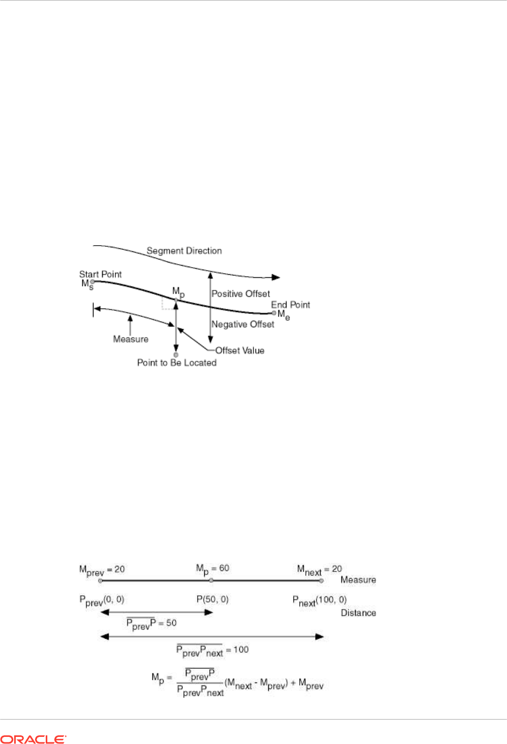
7.1.5 Offset
The offset of a point along a geometric segment is the perpendicular distance between the
point and the geometric segment. Offsets are positive if the points are on the left side along the
segment direction and are negative if they are on the right side. Points are on a geometric
segment if their offsets to the segment are zero.
The unit of measurement for an offset is the same as for the coordinate system associated with
the geometric segment. For geodetic data, the default unit of measurement is meters.
Figure 7-2 shows how a point can be located along a geometric segment with measure and
offset information. By assigning an offset together with a measure, it is possible to locate not
only points that are on the geometric segment, but also points that are perpendicular to the
geometric segment.
Figure 7-2 Describing a Point Along a Segment with a Measure and an Offset
7.1.6 Measure Populating
Any unassigned measures of a geometric segment are automatically populated based upon
their distance distribution. This is done before any LRS operations for geometric segments with
unknown measures (NULL in Oracle Spatial). The resulting geometric segments from any LRS
operations return the measure information associated with geometric segments. The measure
of a point on the geometric segment can be obtained based upon a linear mapping relationship
between its previous and next known measures or locations. See the algorithm representation
in Figure 7-3 and the example in Figure 7-4.
Figure 7-3 Measures, Distances, and Their Mapping Relationship
Chapter 7
LRS Terms and Concepts
7-4

Figure 7-4 Measure Populating of a Geometric Segment
Measures are evenly spaced between assigned measures. However, the assigned measures
for points of interest on a geometric segment do not need to be evenly spaced. This could
eliminate the problem of error accumulation and account for inaccuracy of data source.
Moreover, the assigned measures do not even need to reflect actual distances (for example,
they can reflect estimated driving time); they can be any valid values within the measure range.
Figure 7-5 shows the measure population that results when assigned measure values are not
proportional and reflect widely varying gaps.
Figure 7-5 Measure Populating with Disproportional Assigned Measures
In all cases, measure populating is done in an incremental fashion along the segment
direction. This improves the performance of current and subsequent LRS operations.
7.1.7 Measure Range of a Geometric Segment
The start and end measures of a geometric segment define the linear measure range of the
geometric segment. Any valid LRS measures of a geometric segment must fall within its linear
measure range.
7.1.8 Projection
The projection of a point along a geometric segment is the point on the geometric segment
with the minimum distance to the specified point. The measure information of the resulting
point is also returned in the point geometry.
7.1.9 LRS Point
LRS points are points with linear measure information along a geometric segment. A valid
LRS point is a point geometry with measure information.
Chapter 7
LRS Terms and Concepts
7-5

All LRS point data must be stored in the SDO_ELEM_INFO_ARRAY and
SDO_ORDINATE_ARRAY, and cannot be stored in the SDO_POINT field in the
SDO_GEOMETRY definition of the point.
7.1.10 Linear Features
Linear features are any spatial objects that can be treated as a logical set of linear segments.
Examples of linear features are highways in transportation applications and pipelines in utility
industry applications. The relationship of linear features, geometric segments, and LRS points
is shown in Figure 7-6, where a single linear feature consists of three geometric segments, and
three LRS points are shown on the first segment.
Figure 7-6 Linear Feature, Geometric Segments, and LRS Points
7.1.11 Measures with Multiline Strings and Polygons with Holes
With a multiline string or polygon with hole LRS geometry, the
SDO_LRS.DEFINE_GEOM_SEGMENT procedure and
SDO_LRS.CONVERT_TO_LRS_GEOM function by default assign the same measure value to
the end point of one segment and the start point (separated by a gap) of the next segment,
although you can later assign different measure values to points. Thus, by default there will
duplicate measure values in different segments for such geometries. In such cases, LRS
subprograms use the first point with a specified measure, except when doing so would result in
an invalid geometry.
For example, assume that in a multiline string LRS geometry, the first segment is from
measures 0 through 100 and the second segment is from measures 100 through 150. If you
use the SDO_LRS.LOCATE_PT function to find the point at measure 100, the returned point
will be at measure 100 in the first segment. If you use the
SDO_LRS.CLIP_GEOM_SEGMENT, SDO_LRS.DYNAMIC_SEGMENT, or
SDO_LRS.OFFSET_GEOM_SEGMENT function to return the geometry object between
measures 75 and 125, the result is a multiline string geometry consisting of two segments. If
you use the same function to return the geometry object between measures 100 and 125, the
point at measure 100 in the first segment is ignored, and the result is a line string along the
second segment from measures 100 through 125.
7.2 LRS Data Model
The Oracle Spatial LRS data model incorporates measure information into its geometry
representation at the point level.
Chapter 7
LRS Data Model
7-6

The measure information is directly integrated into the Oracle Spatial model. To accomplish
this, an additional measure dimension must be added to the Oracle Spatial metadata.
Oracle Spatial LRS support affects the spatial metadata and data (the geometries).
Example 7-1 shows how a measure dimension can be added to two-dimensional geometries in
the spatial metadata. The measure dimension must be the last element of the
SDO_DIM_ARRAY in a spatial object definition (shown in bold in Example 7-1).
Figure 7-7 Creating a Geometric Segment
In Figure 7-7, the geometric segment has the following definition (with measure values
underlined):
SDO_GEOMETRY(3302, NULL, NULL,
SDO_ELEM_INFO_ARRAY(1,2,1),
SDO_ORDINATE_ARRAY(5,10,0, 20,5,NULL, 35,10,NULL, 55,10,100))
Whenever a geometric segment is defined, its start and end measures must be defined or
derived from some existing geometric segment. The unsigned measures of all shape points on
a geometric segment will be automatically populated.
The SDO_GTYPE of any point geometry used with an LRS function must be 3301.
Example 7-1 Including LRS Measure Dimension in Spatial Metadata
INSERT INTO user_sdo_geom_metadata
(TABLE_NAME,
COLUMN_NAME,
DIMINFO,
SRID)
VALUES(
'LRS_ROUTES',
'GEOMETRY',
SDO_DIM_ARRAY (
SDO_DIM_ELEMENT('X', 0, 20, 0.005),
SDO_DIM_ELEMENT('Y', 0, 20, 0.005),
SDO_DIM_ELEMENT('M', 0, 100, 0.005)),
NULL);
After adding the new measure dimension, geometries with measure information such as
geometric segments and LRS points can be represented. An example of creating a geometric
segment with three line segments is shown in Figure 7-7.
7.3 Indexing of LRS Data
If LRS data has four dimensions (three plus the M dimension) and if you need to index all three
non-measure dimensions, you must use a spatial R-tree index to index the data.
You must also specify PARAMETERS('sdo_indx_dims=3') in the CREATE INDEX statement to
ensure that the first three dimensions are indexed. Note, however, that if you specify an
sdo_indx_dims
value of 3 or higher, only those operators listed in Three-Dimensional Spatial
Objects as considering all three dimensions can be used on the indexed geometries; the other
Chapter 7
Indexing of LRS Data
7-7

operators described in Spatial Operators cannot be used. (The default value for the
sdo_indx_dims
keyword is 2, which would cause only the first two dimensions to be indexed.)
For example, if the dimensions are X, Y, Z, and M, specify
sdo_indx_dims=3
to index the X, Y,
and Z dimensions, but not the measure (M) dimension. Do not include the measure dimension
in a spatial index, because this causes additional processing overhead and produces no
benefit.
Information about the CREATE INDEX statement and its parameters and keywords is in SQL
Statements for Indexing Spatial Data.
7.4 3D Formats of LRS Functions
Most LRS functions have formats that end in _3D: for example,
DEFINE_GEOM_SEGMENT_3D, CLIP_GEOM_SEGMENT_3D, FIND_MEASURE_3D, and
LOCATE_PT_3D. If a function has a 3D format, it is identified in the Usage Notes for the
function’s reference topic.
The 3D formats are supported only for line string and multiline string geometries. (They are not
supported for polygons, arcs, or circles.) The 3D formats should be used only when the
geometry object has four dimensions and the fourth dimension is the measure (for example, X,
Y, Z, and M), and only when you want the function to consider the first three dimensions (for
example, X, Y, and Z). If the standard format of a function (that is, without the _3D) is used on
a geometry with four dimensions, the function considers only the first two dimensions (for
example, X and Y).
For example, the following format considers the X, Y, and Z dimensions of the specified GEOM
object in performing the clip operation:
SELECT SDO_LRS.CLIP_GEOM_SEGMENT_3D(a.geom, m.diminfo, 5, 10)
FROM routes r, user_sdo_geom_metadata m
WHERE m.table_name = 'ROUTES' AND m.column_name = 'GEOM'
AND r.route_id = 1;
However, the following format considers only the X and Y dimensions, and ignores the Z
dimension, of the specified GEOM object in performing the clip operation:
SELECT SDO_LRS.CLIP_GEOM_SEGMENT(a.geom, m.diminfo, 5, 10)
FROM routes r, user_sdo_geom_metadata m
WHERE m.table_name = 'ROUTES' AND m.column_name = 'GEOM'
AND r.route_id = 1;
The parameters for the standard and 3D formats of any function are the same, and the Usage
Notes apply to both formats.
If the parameters for an LRS function include both a line (or multiline) string and a point (LRS
point), both the line string and the point must have the same number of dimensions. For
example:
• For the SDO_LRS.PROJECT_PT function, the input
geom_segment
(line) must have two
dimensions (X.Y) plus the measure dimension, and the the input
point
point must be a
two-dimensional LRS point geometry with a measure dimension (SDO_GTYPE = 3301).
(This is the case in the example for that function.)
• For the SDO_LRS.PROJECT_PT_3D function. the input
geom_segment
must have three
dimensions (X,Y,Z) plus the measure dimension, and the input
point
point must be a
three-dimensional LRS point geometry with a measure dimension (SDO_GTYPE = 3401).
Chapter 7
3D Formats of LRS Functions
7-8

7.5 LRS Operations
This topic describes several linear referencing operations supported by the Oracle Spatial LRS
API.
• Defining a Geometric Segment
• Redefining a Geometric Segment
• Clipping a Geometric Segment (Dynamic Segmentation)
• Splitting a Geometric Segment
• Concatenating Geometric Segments
• Scaling a Geometric Segment
• Offsetting a Geometric Segment
• Locating a Point on a Geometric Segment
• Projecting a Point onto a Geometric Segment
• Converting LRS Geometries
7.5.1 Defining a Geometric Segment
There are two ways to create a geometric segment with measure information:
• Construct a geometric segment and assign measures explicitly.
• Define a geometric segment with specified start and end, and any other measures, in an
ascending or descending order. Measures of shape points with unknown (unassigned)
measures (null values) in the geometric segment will be automatically populated according
to their locations and distance distribution.
Figure 7-8 shows different ways of defining a geometric segment:
Figure 7-8 Defining a Geometric Segment
Chapter 7
LRS Operations
7-9

An LRS segment must be defined (or must already exist) before any LRS operations can
proceed. That is, the start, end, and any other assigned measures must be present to derive
the location from a specified measure. The measure information of intermediate shape points
will automatically be populated if measure values are not assigned.
7.5.2 Redefining a Geometric Segment
You can redefine a geometric segment to replace the existing measures of all shape points
between the start and end point with automatically calculated measures. Redefining a segment
can be useful if errors have been made in one or more explicit measure assignments, and you
want to start over with proportionally assigned measures.
Figure 7-9 shows the redefinition of a segment where the existing (before) assigned measure
values are not proportional and reflect widely varying gaps.
Figure 7-9 Redefining a Geometric Segment
After the segment redefinition in Figure 7-9, the populated measures reflect proportional
distances along the segment.
7.5.3 Clipping a Geometric Segment (Dynamic Segmentation)
You can clip a geometric segment to create a new geometric segment out of an existing
geometric segment, as shown in Figure 7-10, part a.
Figure 7-10 Clipping, Splitting, and Concatenating Geometric Segments
Chapter 7
LRS Operations
7-10

In Figure 7-10, part a, a segment is created from part of a larger segment. The new segment
has its own start and end points, and the direction is the same as in the original larger
segment.
Clipping segments enables you to perform dynamic segmentation, where you clip the line at
specific measure values. A scenario for such usage would be creating a table of road
conditions, where for a given road, some segments are designated as in good condition and
other segments are designated as in bad condition. For example, the segment between
measures 100 and 120 might be in good condition, but the segment between measures 120
and 125 might be in poor condition. See the reference information for the synonymous
functions SDO_LRS.CLIP_GEOM_SEGMENT and SDO_LRS.DYNAMIC_SEGMENT.
7.5.4 Splitting a Geometric Segment
You can create two new geometric segments by splitting a geometric segment, as shown in the
figure in Clipping a Geometric Segment (Dynamic Segmentation), part b. The direction of each
new segment is the same as in the original segment.
Note:
In Clipping a Geometric Segment (Dynamic Segmentation) and other topics, small
gaps between segments are used in illutrations of segment splitting and
concatenation. Each gap simply reinforces the fact that two different segments are
involved. However, the two segments (such as segment 1 and segment 2 in Clipping
a Geometric Segment (Dynamic Segmentation), parts b and c) are actually
connected. The tolerance (see Tolerance) is considered in determining whether or
not segments are connected.
7.5.5 Concatenating Geometric Segments
You can create a new geometric segment by concatenating two geometric segments, as
shown in part c of the figure in Clipping a Geometric Segment (Dynamic Segmentation). The
geometric segments do not need to be spatially connected, although they are connected in the
illustration in part c of that figure. (If the segments are not spatially connected, the
concatenated result is a multiline string.) The measures of the second geometric segment are
shifted so that the end measure of the first segment is the same as the start measure of the
second segment. The direction of the segment resulting from the concatenation is the same as
in the two original segments.
Measure assignments for the clipping, splitting, and concatenating operations in the figure in
Clipping a Geometric Segment (Dynamic Segmentation) are shown in the following figure.
Measure information and segment direction are preserved in a consistent manner. The
assignment is done automatically when the operations have completed.
Chapter 7
LRS Operations
7-11

Figure 7-11 Measure Assignment in Geometric Segment Operations
The direction of the geometric segment resulting from concatenation is always the direction of
the first segment (
geom_segment1
in the call to the
SDO_LRS.CONCATENATE_GEOM_SEGMENTS function), as shown in the following figure.
Figure 7-12 Segment Direction with Concatenation
In addition to explicitly concatenating two connected segments using the
SDO_LRS.CONCATENATE_GEOM_SEGMENTS function, you can perform aggregate
concatenation: that is, you can concatenate all connected geometric segments in a column
(layer) using the SDO_AGGR_LRS_CONCAT spatial aggregate function. (See the description
and example of the SDO_AGGR_LRS_CONCAT spatial aggregate function in Spatial
Aggregate Functions.)
Chapter 7
LRS Operations
7-12

7.5.6 Scaling a Geometric Segment
You can create a new geometric segment by performing a linear scaling operation on a
geometric segment. Figure 7-13 shows the mapping relationship for geometric segment
scaling.
Figure 7-13 Scaling a Geometric Segment
In general, scaling a geometric segment only involves rearranging measures of the newly
created geometric segment. However, if the scaling factor is negative, the order of the shape
points needs to be reversed so that measures will increase along the geometric segment's
direction (which is defined by the order of the shape points).
A scale operation can perform any combination of the following operations:
• Translating (shifting) measure information. (For example, add the same value to Ms and
Me to get M's and M'e.)
• Reversing measure information. (Let M's = Me, M'e = Ms, and Mshift = 0.)
• Performing simple scaling of measure information. (Let Mshift = 0.)
For examples of these operations, see the Usage Notes and Examples for
theSDO_LRS.SCALE_GEOM_SEGMENT, SDO_LRS.TRANSLATE_MEASURE,
SDO_LRS.REVERSE_GEOMETRY, and SDO_LRS.REDEFINE_GEOM_SEGMENT
subprograms in SDO_LRS Package (Linear Referencing System) .
7.5.7 Offsetting a Geometric Segment
You can create a new geometric segment by performing an offsetting operation on a geometric
segment. Figure 7-14 shows the mapping relationship for geometric segment offsetting.
Figure 7-14 Offsetting a Geometric Segment
Chapter 7
LRS Operations
7-13

In the offsetting operation shown in Figure 7-14, the resulting geometric segment is offset by 5
units from the specified start and end measures of the original segment.
For more information, see the Usage Notes and Examples for the
SDO_LRS.OFFSET_GEOM_SEGMENT function in SDO_LRS Package (Linear Referencing
System) .
7.5.8 Locating a Point on a Geometric Segment
You can find the position of a point described by a measure and an offset on a geometric
segment (see Figure 7-15).
Figure 7-15 Locating a Point Along a Segment with a Measure and an Offset
There is always a unique location with a specific measure on a geometric segment. Ambiguity
arises when offsets are given and the points described by the measures fall on shape points of
the geometric segment (see Figure 7-16).
Figure 7-16 Ambiguity in Location Referencing with Offsets
Chapter 7
LRS Operations
7-14

As shown in Figure 7-16, an offset arc of a shape point on a geometric segment is an arc on
which all points have the same minimum distance to the shape point. As a result, all points on
the offset arc are represented by the same (measure, offset) pair. To resolve this one-to-many
mapping problem, the middle point on the offset arc is returned.
7.5.9 Projecting a Point onto a Geometric Segment
You can find the projection point of a point with respect to a geometric segment. The point to
be projected can be on or off the segment. If the point is on the segment, the point and its
projection point are the same.
Projection is a reverse operation of the point-locating operation shown in Figure 7-15. Similar
to a point-locating operation, all points on the offset arc of a shape point will have the same
projection point (that is, the shape point itself), measure, and offset (see Figure 7-16). If there
are multiple projection points for a point, the first one from the start point is returned (Projection
Point 1 in both illustrations in Figure 7-17).
Figure 7-17 Multiple Projection Points
7.5.10 Converting LRS Geometries
You can convert geometries from standard line string format to LRS format, and the reverse.
The main use of conversion functions will probably occur if you have a large amount of existing
line string data, in which case conversion is a convenient alternative to creating all of the LRS
segments manually. However, if you need to convert LRS segments to standard line strings for
certain applications, that capability is provided also.
Functions are provided to convert:
• Individual line strings or points
For conversion from standard format to LRS format, a measure dimension (named M by
default) is added, and measure information is provided for each point. For conversion from
LRS format to standard format, the measure dimension and information are removed. In
both cases, the dimensional information (DIMINFO) metadata in the
USER_SDO_GEOM_METADATA view is not affected.
• Layers (all geometries in a column)
For conversion from standard format to LRS format, a measure dimension (named M by
default) is added, but no measure information is provided for each point. For conversion
from LRS format to standard format, the measure dimension and information are removed.
In both cases, the dimensional information (DIMINFO) metadata in the
USER_SDO_GEOM_METADATA view is modified as needed.
• Dimensional information (DIMINFO)
Chapter 7
LRS Operations
7-15

The dimensional information (DIMINFO) metadata in the USER_SDO_GEOM_METADATA
view is modified as needed. For example, converting a standard dimensional array with X
and Y dimensions (SDO_DIM_ELEMENT) to an LRS dimensional array causes an M
dimension (SDO_DIM_ELEMENT) to be added.
Figure 7-18 shows the addition of measure information when a standard line string is
converted to an LRS line string (using the SDO_LRS.CONVERT_TO_LRS_GEOM function).
The measure dimension values are underlined in Figure 7-18.
Figure 7-18 Conversion from Standard to LRS Line String
For conversions of point geometries, the SDO_POINT attribute (described in SDO_POINT) in
the returned geometry is affected as follows:
• If a standard point is converted to an LRS point, the SDO_POINT attribute information in
the input geometry is used to set the SDO_ELEM_INFO and SDO_ORDINATES attributes
(described in SDO_ELEM_INFO and SDO_ORDINATES) in the resulting geometry, and
the SDO_POINT attribute in the resulting geometry is set to null.
• If an LRS point is converted to a standard point, the information in the SDO_ELEM_INFO
and SDO_ORDINATES attributes (described in SDO_ELEM_INFO and
SDO_ORDINATES) in the input geometry is used to set the SDO_POINT attribute
information in the resulting geometry, and the SDO_ELEM_INFO and SDO_ORDINATES
attributes in the resulting geometry are set to null.
The conversion functions are listed in SDO_LRS Package (Linear Referencing System) . See
also the reference information in SDO_LRS Package (Linear Referencing System) about each
conversion function.
7.6 Tolerance Values with LRS Functions
Many LRS functions require that you specify a tolerance value or one or more dimensional
arrays.
Thus, you can control whether to specify a single tolerance value for all non-measure
dimensions or to use the tolerance associated with each non-measure dimension in the
dimensional array or arrays. The tolerance is applied only to the geometry portion of the data,
not to the measure dimension. The tolerance value for geodetic data is in meters, and for non-
geodetic data it is in the unit of measurement associated with the data. (For a detailed
discussion of tolerance, see Tolerance.)
Be sure that the tolerance value used is appropriate to the data and your purpose. If the results
of LRS functions seem imprecise or incorrect, you may need to specify a smaller tolerance
value.
For clip operations (see Clipping a Geometric Segment) and offset operations (see Offsetting a
Geometric Segment), if the returned segment has any shape points within the tolerance value
of the input geometric segment from what would otherwise be the start point or end point of the
returned segment, the shape point is used as the start point or end point of the returned
Chapter 7
Tolerance Values with LRS Functions
7-16

segment. This is done to ensure that the resulting geometry does not contain any redundant
vertices, which would cause the geometry to be invalid. For example, assume that the
tolerance associated with the geometric segment (non-geodetic data) in Figure 7-19 is 0.5.
Figure 7-19 Segment for Clip Operation Affected by Tolerance
If you request a clip operation to return the segment between measure values 0 (the start
point) and 61.5 in Figure 7-19, and if the distance between the points associated with measure
values 61.5 and 61.257 is less than the 0.5 tolerance value, the end point of the returned
segment is (35, 10, 61.257).
7.7 Example of LRS Functions
This section presents a simplified example that uses LRS functions.
It refers to concepts that are explained in this chapter and uses functions documented in
SDO_LRS Package (Linear Referencing System) .
This example uses the road that is illustrated in Figure 7-20.
Figure 7-20 Simplified LRS Example: Highway
0 1 2 3 4 5 6 7 8 9 10 11 12 13 14 15
1
2
3
4
5
6
7
8
9
10
11
12
13
14
15
Route1 (start)
Route1 (end)
Exit 1
Exit 2
Exit 3
Exit 4
Exit 5
Exit 6
Segment
Direction
In Figure 7-20, the highway (Route 1) starts at point 2,2 and ends at point 5,14, follows the
path shown, and has six entrance-exit points (Exit 1 through Exit 6). For simplicity, each unit on
the graph represents one unit of measure, and thus the measure from start to end is 27 (the
segment from Exit 5 to Exit 6 being the hypotenuse of a 3-4-5 right triangle).
Each row in Table 7-1 lists an actual highway-related feature and the LRS feature that
corresponds to it or that can be used to represent it.
Chapter 7
Example of LRS Functions
7-17

Table 7-1 Highway Features and LRS Counterparts
Highway Feature LRS Feature
Named route, road, or street LRS segment, or linear feature (logical set of
segments)
Mile or kilometer marker Measure
Accident reporting and location tracking SDO_LRS.LOCATE_PT function
Construction zone (portion of a road) SDO_LRS.CLIP_GEOM_SEGMENT function
Road extension (adding at the beginning or end) or
combination (designating or renaming two roads that
meet as one road)
SDO_LRS.CONCATENATE_GEOM_SEGMEN
TS function
Road reconstruction or splitting (resulting in two
named roads from one named road)
SDO_LRS.SPLIT_GEOM_SEGMENT
procedure
Finding the closest point on the road to a point off the
road (such as a building)
SDO_LRS.PROJECT_PT function
Guard rail or fence alongside a road SDO_LRS.OFFSET_GEOM_SEGMENT
function
Example 7-2 does the following:
• Creates a table to hold the segment depicted in Figure 7-20
• Inserts the definition of the highway depicted in Figure 7-20 into the table
• Inserts the necessary metadata into the USER_SDO_GEOM_METADATA view
• Uses PL/SQL and SQL statements to define the segment and perform operations on it
Example 7-2 Simplified Example: Highway
-- Create a table for routes (highways).
CREATE TABLE lrs_routes (
route_id NUMBER PRIMARY KEY,
route_name VARCHAR2(32),
route_geometry SDO_GEOMETRY);
-- Populate table with just one route for this example.
INSERT INTO lrs_routes VALUES(
1,
'Route1',
SDO_GEOMETRY(
3302, -- line string, 3 dimensions: X,Y,M
NULL,
NULL,
SDO_ELEM_INFO_ARRAY(1,2,1), -- one line string, straight segments
SDO_ORDINATE_ARRAY(
2,2,0, -- Start point - Exit1; 0 is measure from start.
2,4,2, -- Exit2; 2 is measure from start.
8,4,8, -- Exit3; 8 is measure from start.
12,4,12, -- Exit4; 12 is measure from start.
12,10,NULL, -- Not an exit; measure automatically calculated and filled.
8,10,22, -- Exit5; 22 is measure from start.
5,14,27) -- End point (Exit6); 27 is measure from start.
)
);
-- Update the spatial metadata.
INSERT INTO user_sdo_geom_metadata
Chapter 7
Example of LRS Functions
7-18

(TABLE_NAME,
COLUMN_NAME,
DIMINFO,
SRID)
VALUES (
'lrs_routes',
'route_geometry',
SDO_DIM_ARRAY( -- 20X20 grid
SDO_DIM_ELEMENT('X', 0, 20, 0.005),
SDO_DIM_ELEMENT('Y', 0, 20, 0.005),
SDO_DIM_ELEMENT('M', 0, 20, 0.005) -- Measure dimension
),
NULL -- SRID
);
-- Create the spatial index.
CREATE INDEX lrs_routes_idx ON lrs_routes(route_geometry)
INDEXTYPE IS MDSYS.SPATIAL_INDEX_V2;
-- Test the LRS procedures.
DECLARE
geom_segment SDO_GEOMETRY;
line_string SDO_GEOMETRY;
dim_array SDO_DIM_ARRAY;
result_geom_1 SDO_GEOMETRY;
result_geom_2 SDO_GEOMETRY;
result_geom_3 SDO_GEOMETRY;
BEGIN
SELECT a.route_geometry into geom_segment FROM lrs_routes a
WHERE a.route_name = 'Route1';
SELECT m.diminfo into dim_array from
user_sdo_geom_metadata m
WHERE m.table_name = 'LRS_ROUTES' AND m.column_name = 'ROUTE_GEOMETRY';
-- Define the LRS segment for Route1. This will populate any null measures.
-- No need to specify start and end measures, because they are already defined
-- in the geometry.
SDO_LRS.DEFINE_GEOM_SEGMENT (geom_segment, dim_array);
SELECT a.route_geometry INTO line_string FROM lrs_routes a
WHERE a.route_name = 'Route1';
-- Split Route1 into two segments.
SDO_LRS.SPLIT_GEOM_SEGMENT(line_string,dim_array,5,result_geom_1,result_geom_2);
-- Concatenate the segments that were just split.
result_geom_3 := SDO_LRS.CONCATENATE_GEOM_SEGMENTS(result_geom_1, dim_array,
result_geom_2, dim_array);
-- Update and insert geometries into table, to display later.
UPDATE lrs_routes a SET a.route_geometry = geom_segment
WHERE a.route_id = 1;
INSERT INTO lrs_routes VALUES(
11,
'result_geom_1',
result_geom_1
);
INSERT INTO lrs_routes VALUES(
12,
Chapter 7
Example of LRS Functions
7-19

'result_geom_2',
result_geom_2
);
INSERT INTO lrs_routes VALUES(
13,
'result_geom_3',
result_geom_3
);
END;
/
-- First, display the data in the LRS table.
SELECT route_id, route_name, route_geometry FROM lrs_routes;
-- Are result_geom_1 and result_geom2 connected?
SELECT SDO_LRS.CONNECTED_GEOM_SEGMENTS(a.route_geometry,
b.route_geometry, 0.005)
FROM lrs_routes a, lrs_routes b
WHERE a.route_id = 11 AND b.route_id = 12;
-- Is the Route1 segment valid?
SELECT SDO_LRS.VALID_GEOM_SEGMENT(route_geometry)
FROM lrs_routes WHERE route_id = 1;
-- Is 50 a valid measure on Route1? (Should return FALSE; highest Route1 measure is 27.)
SELECT SDO_LRS.VALID_MEASURE(route_geometry, 50)
FROM lrs_routes WHERE route_id = 1;
-- Is the Route1 segment defined?
SELECT SDO_LRS.IS_GEOM_SEGMENT_DEFINED(route_geometry)
FROM lrs_routes WHERE route_id = 1;
-- How long is Route1?
SELECT SDO_LRS.GEOM_SEGMENT_LENGTH(route_geometry)
FROM lrs_routes WHERE route_id = 1;
-- What is the start measure of Route1?
SELECT SDO_LRS.GEOM_SEGMENT_START_MEASURE(route_geometry)
FROM lrs_routes WHERE route_id = 1;
-- What is the end measure of Route1?
SELECT SDO_LRS.GEOM_SEGMENT_END_MEASURE(route_geometry)
FROM lrs_routes WHERE route_id = 1;
-- What is the start point of Route1?
SELECT SDO_LRS.GEOM_SEGMENT_START_PT(route_geometry)
FROM lrs_routes WHERE route_id = 1;
-- What is the end point of Route1?
SELECT SDO_LRS.GEOM_SEGMENT_END_PT(route_geometry)
FROM lrs_routes WHERE route_id = 1;
-- Translate (shift measure values) (+10).
-- First, display the original segment; then, translate.
SELECT a.route_geometry FROM lrs_routes a WHERE a.route_id = 1;
SELECT SDO_LRS.TRANSLATE_MEASURE(a.route_geometry, m.diminfo, 10)
FROM lrs_routes a, user_sdo_geom_metadata m
WHERE m.table_name = 'LRS_ROUTES' AND m.column_name = 'ROUTE_GEOMETRY'
AND a.route_id = 1;
-- Redefine geometric segment to "convert" miles to kilometers
Chapter 7
Example of LRS Functions
7-20

DECLARE
geom_segment SDO_GEOMETRY;
dim_array SDO_DIM_ARRAY;
BEGIN
SELECT a.route_geometry into geom_segment FROM lrs_routes a
WHERE a.route_name = 'Route1';
SELECT m.diminfo into dim_array from
user_sdo_geom_metadata m
WHERE m.table_name = 'LRS_ROUTES' AND m.column_name = 'ROUTE_GEOMETRY';
-- "Convert" mile measures to kilometers (27 * 1.609 = 43.443).
SDO_LRS.REDEFINE_GEOM_SEGMENT (geom_segment,
dim_array,
0, -- Zero starting measure: LRS segment starts at start of route.
43.443); -- End of LRS segment. 27 miles = 43.443 kilometers.
-- Update and insert geometries into table, to display later.
UPDATE lrs_routes a SET a.route_geometry = geom_segment
WHERE a.route_id = 1;
END;/
-- Display the redefined segment, with all measures "converted."
SELECT a.route_geometry FROM lrs_routes a WHERE a.route_id = 1;
-- Clip a piece of Route1.
SELECT SDO_LRS.CLIP_GEOM_SEGMENT(route_geometry, 5, 10)
FROM lrs_routes WHERE route_id = 1;
-- Point (9,3,NULL) is off the road; should return (9,4,9).
SELECT SDO_LRS.PROJECT_PT(route_geometry,
SDO_GEOMETRY(3301, NULL, NULL,
SDO_ELEM_INFO_ARRAY(1, 1, 1),
SDO_ORDINATE_ARRAY(9, 3, NULL)) )
FROM lrs_routes WHERE route_id = 1;
-- Return the measure of the projected point.
SELECT SDO_LRS.GET_MEASURE(
SDO_LRS.PROJECT_PT(a.route_geometry, m.diminfo,
SDO_GEOMETRY(3301, NULL, NULL,
SDO_ELEM_INFO_ARRAY(1, 1, 1),
SDO_ORDINATE_ARRAY(9, 3, NULL)) ),
m.diminfo )
FROM lrs_routes a, user_sdo_geom_metadata m
WHERE m.table_name = 'LRS_ROUTES' AND m.column_name = 'ROUTE_GEOMETRY'
AND a.route_id = 1;
-- Is point (9,3,NULL) a valid LRS point? (Should return TRUE.)
SELECT SDO_LRS.VALID_LRS_PT(
SDO_GEOMETRY(3301, NULL, NULL,
SDO_ELEM_INFO_ARRAY(1, 1, 1),
SDO_ORDINATE_ARRAY(9, 3, NULL)),
m.diminfo)
FROM lrs_routes a, user_sdo_geom_metadata m
WHERE m.table_name = 'LRS_ROUTES' AND m.column_name = 'ROUTE_GEOMETRY'
AND a.route_id = 1;
-- Locate the point on Route1 at measure 9, offset 0.
SELECT SDO_LRS.LOCATE_PT(route_geometry, 9, 0)
FROM lrs_routes WHERE route_id = 1;
Chapter 7
Example of LRS Functions
7-21

Example 7-3 shows the output of the SELECT statements in Example 7-2.
Example 7-3 Simplified Example: Output of SELECT Statements
SQL> -- First, display the data in the LRS table.
SQL> SELECT route_id, route_name, route_geometry FROM lrs_routes;
ROUTE_ID ROUTE_NAME
---------- --------------------------------
ROUTE_GEOMETRY(SDO_GTYPE, SDO_SRID, SDO_POINT(X, Y, Z), SDO_ELEM_INFO, SDO_ORDIN
--------------------------------------------------------------------------------
1 Route1
SDO_GEOMETRY(3302, NULL, NULL, SDO_ELEM_INFO_ARRAY(1, 2, 1), SDO_ORDINATE_ARRAY(
2, 2, 0, 2, 4, 2, 8, 4, 8, 12, 4, 12, 12, 10, 18, 8, 10, 22, 5, 14, 27))
11 result_geom_1
SDO_GEOMETRY(3302, NULL, NULL, SDO_ELEM_INFO_ARRAY(1, 2, 1), SDO_ORDINATE_ARRAY(
2, 2, 0, 2, 4, 2, 5, 4, 5))
12 result_geom_2
ROUTE_ID ROUTE_NAME
---------- --------------------------------
ROUTE_GEOMETRY(SDO_GTYPE, SDO_SRID, SDO_POINT(X, Y, Z), SDO_ELEM_INFO, SDO_ORDIN
--------------------------------------------------------------------------------
SDO_GEOMETRY(3302, NULL, NULL, SDO_ELEM_INFO_ARRAY(1, 2, 1), SDO_ORDINATE_ARRAY(
5, 4, 5, 8, 4, 8, 12, 4, 12, 12, 10, 18, 8, 10, 22, 5, 14, 27))
13 result_geom_3
SDO_GEOMETRY(3302, NULL, NULL, SDO_ELEM_INFO_ARRAY(1, 2, 1), SDO_ORDINATE_ARRAY(
2, 2, 0, 2, 4, 2, 5, 4, 5, 8, 4, 8, 12, 4, 12, 12, 10, 18, 8, 10, 22, 5, 14, 27)
)
SQL> -- Are result_geom_1 and result_geom2 connected?
SQL> SELECT SDO_LRS.CONNECTED_GEOM_SEGMENTS(a.route_geometry,
2 b.route_geometry, 0.005)
3 FROM lrs_routes a, lrs_routes b
4 WHERE a.route_id = 11 AND b.route_id = 12;
SDO_LRS.CONNECTED_GEOM_SEGMENTS(A.ROUTE_GEOMETRY,B.ROUTE_GEOMETRY,0.005)
--------------------------------------------------------------------------------
TRUE
SQL> -- Is the Route1 segment valid?
SQL> SELECT SDO_LRS.VALID_GEOM_SEGMENT(route_geometry)
2 FROM lrs_routes WHERE route_id = 1;
SDO_LRS.VALID_GEOM_SEGMENT(ROUTE_GEOMETRY)
--------------------------------------------------------------------------------
TRUE
SQL> -- Is 50 a valid measure on Route1? (Should return FALSE; highest Route1 measure is
27.)
SQL> SELECT SDO_LRS.VALID_MEASURE(route_geometry, 50)
2 FROM lrs_routes WHERE route_id = 1;
SDO_LRS.VALID_MEASURE(ROUTE_GEOMETRY,50)
--------------------------------------------------------------------------------
FALSE
SQL> -- Is the Route1 segment defined?
SQL> SELECT SDO_LRS.IS_GEOM_SEGMENT_DEFINED(route_geometry)
2 FROM lrs_routes WHERE route_id = 1;
Chapter 7
Example of LRS Functions
7-22

SDO_LRS.IS_GEOM_SEGMENT_DEFINED(ROUTE_GEOMETRY)
--------------------------------------------------------------------------------
TRUE
SQL> -- How long is Route1?
SQL> SELECT SDO_LRS.GEOM_SEGMENT_LENGTH(route_geometry)
2 FROM lrs_routes WHERE route_id = 1;
SDO_LRS.GEOM_SEGMENT_LENGTH(ROUTE_GEOMETRY)
-------------------------------------------
27
SQL> -- What is the start measure of Route1?
SQL> SELECT SDO_LRS.GEOM_SEGMENT_START_MEASURE(route_geometry)
2 FROM lrs_routes WHERE route_id = 1;
SDO_LRS.GEOM_SEGMENT_START_MEASURE(ROUTE_GEOMETRY)
--------------------------------------------------
0
SQL> -- What is the end measure of Route1?
SQL> SELECT SDO_LRS.GEOM_SEGMENT_END_MEASURE(route_geometry)
2 FROM lrs_routes WHERE route_id = 1;
SDO_LRS.GEOM_SEGMENT_END_MEASURE(ROUTE_GEOMETRY)
------------------------------------------------
27
SQL> -- What is the start point of Route1?
SQL> SELECT SDO_LRS.GEOM_SEGMENT_START_PT(route_geometry)
2 FROM lrs_routes WHERE route_id = 1;
SDO_LRS.GEOM_SEGMENT_START_PT(ROUTE_GEOMETRY)(SDO_GTYPE, SDO_SRID, SDO_POINT(X,
--------------------------------------------------------------------------------
SDO_GEOMETRY(3301, NULL, NULL, SDO_ELEM_INFO_ARRAY(1, 1, 1), SDO_ORDINATE_ARRAY(
2, 2, 0))
SQL> -- What is the end point of Route1?
SQL> SELECT SDO_LRS.GEOM_SEGMENT_END_PT(route_geometry)
2 FROM lrs_routes WHERE route_id = 1;
SDO_LRS.GEOM_SEGMENT_END_PT(ROUTE_GEOMETRY)(SDO_GTYPE, SDO_SRID, SDO_POINT(X, Y,
--------------------------------------------------------------------------------
SDO_GEOMETRY(3301, NULL, NULL, SDO_ELEM_INFO_ARRAY(1, 1, 1), SDO_ORDINATE_ARRAY(
5, 14, 27))
SQL> -- Translate (shift measure values) (+10).
SQL> -- First, display the original segment; then, translate.
SQL> SELECT a.route_geometry FROM lrs_routes a WHERE a.route_id = 1;
ROUTE_GEOMETRY(SDO_GTYPE, SDO_SRID, SDO_POINT(X, Y, Z), SDO_ELEM_INFO, SDO_ORDIN
--------------------------------------------------------------------------------
SDO_GEOMETRY(3302, NULL, NULL, SDO_ELEM_INFO_ARRAY(1, 2, 1), SDO_ORDINATE_ARRAY(
2, 2, 0, 2, 4, 2, 8, 4, 8, 12, 4, 12, 12, 10, 18, 8, 10, 22, 5, 14, 27))
SQL> SELECT SDO_LRS.TRANSLATE_MEASURE(a.route_geometry, m.diminfo, 10)
2 FROM lrs_routes a, user_sdo_geom_metadata m
3 WHERE m.table_name = 'LRS_ROUTES' AND m.column_name = 'ROUTE_GEOMETRY'
4 AND a.route_id = 1;
SDO_LRS.TRANSLATE_MEASURE(A.ROUTE_GEOMETRY,M.DIMINFO,10)(SDO_GTYPE, SDO_SRID, SD
Chapter 7
Example of LRS Functions
7-23

--------------------------------------------------------------------------------
SDO_GEOMETRY(3302, NULL, NULL, SDO_ELEM_INFO_ARRAY(1, 2, 1), SDO_ORDINATE_ARRAY(
2, 2, 10, 2, 4, 12, 8, 4, 18, 12, 4, 22, 12, 10, 28, 8, 10, 32, 5, 14, 37))
SQL> -- Redefine geometric segment to "convert" miles to kilometers
SQL> DECLARE
2 geom_segment SDO_GEOMETRY;
3 dim_array SDO_DIM_ARRAY;
4
5 BEGIN
6
7 SELECT a.route_geometry into geom_segment FROM lrs_routes a
8 WHERE a.route_name = 'Route1';
9 SELECT m.diminfo into dim_array from
10 user_sdo_geom_metadata m
11 WHERE m.table_name = 'LRS_ROUTES' AND m.column_name = 'ROUTE_GEOMETRY';
12
13 -- "Convert" mile measures to kilometers (27 * 1.609 = 43.443).
14 SDO_LRS.REDEFINE_GEOM_SEGMENT (geom_segment,
15 dim_array,
16 0, -- Zero starting measure: LRS segment starts at start of route.
17 43.443); -- End of LRS segment. 27 miles = 43.443 kilometers.
18
19 -- Update and insert geometries into table, to display later.
20 UPDATE lrs_routes a SET a.route_geometry = geom_segment
21 WHERE a.route_id = 1;
22
23 END;
24 /
PL/SQL procedure successfully completed.
SQL> -- Display the redefined segment, with all measures "converted."
SQL> SELECT a.route_geometry FROM lrs_routes a WHERE a.route_id = 1;
ROUTE_GEOMETRY(SDO_GTYPE, SDO_SRID, SDO_POINT(X, Y, Z), SDO_ELEM_INFO, SDO_ORDIN
--------------------------------------------------------------------------------
SDO_GEOMETRY(3302, NULL, NULL, SDO_ELEM_INFO_ARRAY(1, 2, 1), SDO_ORDINATE_ARRAY(
2, 2, 0, 2, 4, 3.218, 8, 4, 12.872, 12, 4, 19.308, 12, 10, 28.962, 8, 10, 35.398
, 5, 14, 43.443))
SQL> -- Clip a piece of Route1.
SQL> SELECT SDO_LRS.CLIP_GEOM_SEGMENT(route_geometry, 5, 10)
2 FROM lrs_routes WHERE route_id = 1;
SDO_LRS.CLIP_GEOM_SEGMENT(ROUTE_GEOMETRY,5,10)(SDO_GTYPE, SDO_SRID, SDO_POINT(X,
--------------------------------------------------------------------------------
SDO_GEOMETRY(3302, NULL, NULL, SDO_ELEM_INFO_ARRAY(1, 2, 1), SDO_ORDINATE_ARRAY(
5, 4, 5, 8, 4, 8, 10, 4, 10))
SQL> -- Point (9,3,NULL) is off the road; should return (9,4,9).
SQL> SELECT SDO_LRS.PROJECT_PT(route_geometry,
2 SDO_GEOMETRY(3301, NULL, NULL,
3 SDO_ELEM_INFO_ARRAY(1, 1, 1),
4 SDO_ORDINATE_ARRAY(9, 3, NULL)) )
5 FROM lrs_routes WHERE route_id = 1;
SDO_LRS.PROJECT_PT(ROUTE_GEOMETRY,SDO_GEOMETRY(3301,NULL,NULL,SDO_EL
--------------------------------------------------------------------------------
SDO_GEOMETRY(3301, NULL, NULL, SDO_ELEM_INFO_ARRAY(1, 1, 1), SDO_ORDINATE_ARRAY(
9, 4, 9))
Chapter 7
Example of LRS Functions
7-24

SQL> -- Return the measure of the projected point.
SQL> SELECT SDO_LRS.GET_MEASURE(
2 SDO_LRS.PROJECT_PT(a.route_geometry, m.diminfo,
3 SDO_GEOMETRY(3301, NULL, NULL,
4 SDO_ELEM_INFO_ARRAY(1, 1, 1),
5 SDO_ORDINATE_ARRAY(9, 3, NULL)) ),
6 m.diminfo )
7 FROM lrs_routes a, user_sdo_geom_metadata m
8 WHERE m.table_name = 'LRS_ROUTES' AND m.column_name = 'ROUTE_GEOMETRY'
9 AND a.route_id = 1;
SDO_LRS.GET_MEASURE(SDO_LRS.PROJECT_PT(A.ROUTE_GEOMETRY,M.DIMINFO,SDO_GEOM
--------------------------------------------------------------------------------
9
SQL> -- Is point (9,3,NULL) a valid LRS point? (Should return TRUE.)
SQL> SELECT SDO_LRS.VALID_LRS_PT(
2 SDO_GEOMETRY(3301, NULL, NULL,
3 SDO_ELEM_INFO_ARRAY(1, 1, 1),
4 SDO_ORDINATE_ARRAY(9, 3, NULL)),
5 m.diminfo)
6 FROM lrs_routes a, user_sdo_geom_metadata m
7 WHERE m.table_name = 'LRS_ROUTES' AND m.column_name = 'ROUTE_GEOMETRY'
8 AND a.route_id = 1;
SDO_LRS.VALID_LRS_PT(SDO_GEOMETRY(3301,NULL,NULL,SDO_ELEM_INFO_ARRAY
------------------------------------------------------------------------------
TRUE
SQL> -- Locate the point on Route1 at measure 9, offset 0.
SQL> SELECT SDO_LRS.LOCATE_PT(route_geometry, 9, 0)
2 FROM lrs_routes WHERE route_id = 1;
SDO_LRS.LOCATE_PT(ROUTE_GEOMETRY,9,0)(SDO_GTYPE, SDO_SRID, SDO_POINT(X, Y, Z), S
--------------------------------------------------------------------------------
SDO_GEOMETRY(3301, NULL, NULL, SDO_ELEM_INFO_ARRAY(1, 1, 1), SDO_ORDINATE_ARRAY(
9, 4, 9))
Chapter 7
Example of LRS Functions
7-25

8
Location Tracking Server
The Oracle Spatial location tracking server enables you to define regions, track the movement
of objects into or out of those regions, and receive notifications when certain movements occur.
For reference information about location tracking PL/SQL subprograms, see SDO_TRKR
Package (Location Tracking).
• About the Location Tracking Server
As location becomes an increasingly important aspect of our lives, and as location-sensing
devices become ubiquitous, there is an increasing demand for applications to be able to
monitor subscriber location data continuously. The monitoring of the location data may
translate into alerts being generated in the system.
• Location Tracking Set
The location tracking server tracks a set of moving objects against a known set of regions
and generates notifications as required. In this framework, the set of objects and regions is
referred to as a tracking set.
• Data Types for the Location Tracking Server
The PL/SQL subprograms associated with location tracking have parameters of data types
that are specific to the location tracking server.
• Data Structures for the Location Tracking Server
The location tracking server requires the user to specify a tracking set name when the
server is created. Based on this name, additional data structures are created.
• Workflow for the Location Tracking Server
The typical location tracking workflow involves several operations, some required and
others optional.
8.1 About the Location Tracking Server
As location becomes an increasingly important aspect of our lives, and as location-sensing
devices become ubiquitous, there is an increasing demand for applications to be able to
monitor subscriber location data continuously. The monitoring of the location data may
translate into alerts being generated in the system.
For example, a trucking company may want to monitor its network of 10,000 trucks as they
move along their specified routes towards their destinations. They may want to track the
movement of trucks within a specified range of the route and expect notifications to be
generated to detect undesirable deviations the vehicles from their desired routes. Proactive
location-based services (LBSs) generalize such applications that track locations of subscribers
inside or outside a specified region for various purposes, such as location-based advertising
and notifications about friends nearby.
The Oracle Spatial location tracking server provides:
• A simple framework for setting up a location tracking network within the database through
a PL/SQL interface
• An API for continuous location monitoring of objects within a tracking network
8-1

• A queuing mechanism for incoming location updates and tracking requests and for
outgoing relevant notifications, using Oracle Advanced Queuing
• Efficient, continuous location monitoring for thousands of relevant objects within the
database
8.2 Location Tracking Set
The location tracking server tracks a set of moving objects against a known set of regions and
generates notifications as required. In this framework, the set of objects and regions is referred
to as a tracking set.
In the database these are managed in a table with two columns:
region_id NUMBER,
geometry SDO_GEOMETRY
REGION_ID is the primary key for this table, and GEOMETRY is the geometry of the tracking
region.
Several additional structures are created when you create a tracking set. You can create any
number of tracking sets, and each tracking set can have thousands of regions. When a region
is no longer of interest for tracking purposes, it should be deleted from the tracking regions
table.
A set of objects to be tracked also needs to be created. Each object must specify an ID for the
object and a region ID to specify the region in which this object is tracked. That is, each object
can be tracked against one or more tracking regions. An object is created by inserting a tracker
message,
TRACKER_MSG
, into a tracking queue.
A tracker message object specifies the
object_id
,
region_id
, and
operation
. The
operation
parameter has one of the following string values.
•
I
: A notification message is issued every time an object, defined by
object_id
, moves
while inside the region, defined by
region_id
•
O
: A notification message is issued every time an object, defined by
object_id
, moves
while outside the region, defined by
region_id
.
•
T
: A notification message is issued only when the object, defined by
object_id
,
transitions from inside to outside or from outside to inside the region defined by
region_id
.
•
D
: Disables the tracking of an object defined by
object_id
in the region defined by
region_id
. To enable tracking of this object again, another tracking message must be
sent.
After the objects are created and tracking regions configured, new location messages for the
objects can be sent. As objects move in space, their locations change. Every time a new
location message is sent, it is inserted into the location message queue, to be processed by
the location tracking server. Location messages are processed and notification messages are
generated as required. Applications can monitor the notification queue and process the
notification messages whenever new notifications are generated.
The following additional grants are required for a user to run the location tracking server.
GRANT aq_administrator_role, create job, manage scheduler to <USER>; grant
execute on dbms_aq to <USER>;
GRANT execute on dbms_aqadm to <USER>;
GRANT execute on dbms_lock to <USER>;
Chapter 8
Location Tracking Set
8-2

GRANT execute on dbms_aqin to <USER>;
GRANT execute on dbms_aqjms to <USER>;
8.3 Data Types for the Location Tracking Server
The PL/SQL subprograms associated with location tracking have parameters of data types that
are specific to the location tracking server.
These subprograms are documented in the SDO_TRKR Package (Location Tracking). The
specific data types have the following definitions:
• LOCATION_MSG
(object_id INTEGER,
time TIMESTAMP,
x NUMBER,
y NUMBER)
• LOCATION_MSG_ARR
VARRAY(1000) of location_msg
• LOCATION_MSG_PKD
object(arr location_msg_arr)
• NOTIFICATION_MSG
(object_id INTEGER,
region_id INTEGER,
time TIMESTAMP,
x NUMBER,
y NUMBER,
state VARCHAR2(8))
• PROC_MSG
(object_id INTEGER,
time TIMESTAMP,
x NUMBER,
y NUMBER,
region_id INTEGER,
alert_when VARCHAR2(2))
• PROC_MSG_ARR
VARRAY(1000) of proc_msg
• PROC_MSG_PKD
object(arr proc_msg_arr)
• TRACKER_MSG
(object_id INTEGER,
region_id INTEGER,
operation VARCHAR2(2))
8.4 Data Structures for the Location Tracking Server
The location tracking server requires the user to specify a tracking set name when the server is
created. Based on this name, additional data structures are created.
Chapter 8
Data Types for the Location Tracking Server
8-3

• <TS_NAME>_TRACKING_REGIONS (region_id NUMBER, geometry
MDSYS.SDO_GEOMETRY) is a table containing the tracking region polygons defined in
the tracking set <TS_NAME>. Users must insert the polygons into this table after the
server is created. All of the polygons must be geodetic (using SRID 8307) and two
dimensional. The table has a primary key defined on the REGION_ID column.
• <TS_NAME>_TRACKER (object_id NUMBER, region_id NUMBER, queue_no NUMBER,
alert_when VARCHAR2(2)) is a table whose entries map the relationship between an
object and a region in which the object is tracked. The table has a primary key defined on
the OBJECT_ID and REGION_ID columns. This table is managed using the
TRACKER_MSG type; users should not update this table directly.
• <TS_NAME>_TRACKER_QUEUES(num_loc_queues NUMBER, num_trkr_queues
NUMBER) is a table that holds queue information needed by the server. The server
populates and maintains this table; users should never modify this table.
• <TS_NAME>_TRACKER_LOG (message_level VARCHAR2(1), message
VARCHAR2(512), ts TIMESTAMP WITH TIMEZONE) is a table containing log messages
generated by the server. Message level ‘I’ indicates an informational message, and
message level ‘E’ indicates an error message. This table is not dropped when the tracking
set is dropped. However, if a tracking set of the same name is then created, this table is
truncated and reused by the new tracking set.
• <TS_NAME>_NOTIFICATIONS (object_id NUMBER, region_id NUMBER, time
TIMESTAMP, x NUMBER, y NUMBER, state VARCHAR2(8)) is an auxiliary table provided
to users to store messages from the notifications queue. The layout of columns in this table
match that of the NOTIFICATION_MSG type. The X and Y columns are the coordinate that
prompted the notification for object_id in region_id at the time. The STATE column shows if
the point INSIDE or OUTSIDE the region. For tracking types INSIDE and OUTSIDE this
value never changes. For tracking type TRANSITION this column is the state of the object
at the time it generated the notification.
• <TS_NAME>_TRAJECTORY is an auxiliary table not currently used by the location
tracking server.
In addition to these tables, the location tracking server also creates a set of Advanced Queuing
(AQ) objects for managing the location, tracking and notification messages. All of the queues
have a prefix of <TS_NAME>, for example. <TS_NAME>_TRACKER_Q_1 and
<TS_NAME>_LOCATION_Q_1.
8.5 Workflow for the Location Tracking Server
The typical location tracking workflow involves several operations, some required and others
optional.
The typical workflow contains several steps:
1. Create a tracking set.
2. Optionally, show the tracking set tables that were created.
3. Start the tracking set.
4. Optionally, show the queues used by the tracking set.
5. Optionally, show the Scheduler jobs used by the tracking set.
6. Insert polygons for various regions.
7. Create object-region pairs to be tracked.
8. Optionally, show the object-region pairs in the tracking set.
Chapter 8
Workflow for the Location Tracking Server
8-4

9. Send location messages.
10. Optionally, show the location messages that have been sent.
11. Dequeue the notification messages into the notifications table.
12. Optionally, disable the tracking server's object-region pairs.
13. Stop the tracking set.
14. Drop the tracking set.
The following is a simple example of the location tracking server workflow.
Example 8-1 Location Tracking Server Workflow
-- Create a tracking set named sample with one tracker/process
-- queue pair and one location queue.
EXEC sdo_trkr.create_tracking_set('sample', 1, 1);
-- Optional: Show the tracking sets tables that were created
SELECT table_name
FROM user_tables
WHERE table_name LIKE ‘SAMPLE%’
ORDER BY table_name;
TABLE_NAME
----------------------
SAMPLE_LOCATION_QT_1 - AQ queue table for location queue
SAMPLE_NOTIFICATIONS - Auxiliary table to store notification messages
SAMPLE_NOTIFICATION_QT - AQ queue table for the notification queue
SAMPLE_PROC_QT_1 - AQ queue table for the process queue
SAMPLE_TRACKER - Table, will contain object-region tracking pairs
SAMPLE_TRACKER_LOG - Table, contains log messages from the server
SAMPLE_TRACKER_QT_1 - AQ queue table for the tracker queue
SAMPLE_TRACKER_QUEUES - Table, contains tracking sets queue metadata
SAMPLE_TRACKING_REGIONS - Table, will contain the regions geometry
SAMPLE_TRAJECTORY - Table, currently unused
-- Start the tracking set
EXEC sdo_trkr.start_tracking_set(‘sample’);
-- Optional: Show the queues used by the tracking set
SELECT name
FROM user_queues
WHERE name LIKE 'SAMPLE%'
ORDER BY name;
NAME
---------------------
SAMPLE_LOCATION_Q_1
SAMPLE_NOTIFICATION_Q
SAMPLE_PROC_Q_1
SAMPLE_TRACKER_Q_1
-- Optional: Show the scheduler jobs used by the tracking set
SELECT job_name, state
FROM user_scheduler_jobs
WHERE job_name LIKE 'SAMPLE%'
Chapter 8
Workflow for the Location Tracking Server
8-5

ORDER BY job_name;
JOB_NAME STATE
--------------------------
SAMPLE_LOC_JOB_1 RUNNING
SAMPLE_TRKR_JOB_1 RUNNING
-- Insert a polygon for region 1. This polygon must be geodetic (using SRID
8307)
-- and two dimensional. The region may also be a multi-polygon.
INSERT INTO SAMPLE_TRACKING_REGIONS VALUES (1,
MDSYS.SDO_GEOMETRY(2003, 8307, null,
sdo_elem_info_array(1, 1003, 1),
sdo_ordinate_array(0,0, 5,0, 5,5, 0,5, 0,0)));
-- Create two objects, object 1 and 2 that are tracked in region 1.
-- Object 1 sends notification messages when it is inside region 1.
-- Object 2 sends notification messages when it is outside region 1.
EXEC sdo_trkr.send_tracking_msg(
'SAMPLE', mdsys.tracker_msg(1, 1, 'I'));
EXEC sdo_trkr.send_tracking_msg(
'SAMPLE', mdsys.tracker_msg(2, 1, 'O'));
-- Optional: Show the object-region pairs used in the tracking set
SELECT object_id, region_id, alert_when FROM sample_tracker;
OBJECT_ID REGION_ID ALERT_WHEN
---------- ---------- -----------
1 1 I
2 1 O
-- Send 2 location messages.
–- Object 1 moves to (1, 1).
–- Object 2 moves to (8, 8).
EXEC sdo_trkr.send_location_msgs('SAMPLE',
mdsys.location_msg_arr(
mdsys.location_msg(1, '01-AUG-16 01.01.46.000000 PM', 1, 1),
mdsys.location_msg(2, '01-AUG-16 01.02.46.000000 PM', 8, 8)));
-- Optional: Show that 2 notification message were generated
SELECT a.name, b.ready
FROM user_queues a, v$aq b
WHERE a.name='SAMPLE_NOTIFICATION_Q' AND a.qid=b.qid
ORDER BY a.name;
NAME READY
---------------------- ------
SAMPLE_NOTIFICATION_Q 2
-- Dequeue the notification messages into the notifications table
DECLARE
message mdsys.notification_msg;
BEGIN
LOOP
sdo_trkr.get_notification_msg(
tracking_set_name => 'SAMPLE',
message => message,
Chapter 8
Workflow for the Location Tracking Server
8-6

deq_wait =>2); -- wait at most 2 seconds for a message
IF (message IS NULL) THEN
EXIT;
END IF;
INSERT INTO sample_notifications (
object_id, region_id, time, x, y, state)
(SELECT message.object_id, message.region_id,
message.time, message.x, message.y, message.state);
END LOOP;
END;
-- Query the object id, region id, (x, y) coordinate and the objects
-- relationship to the region sorted by the time that was sent with
-- the objects location message.
SELECT object_id, region_id, x, y, state
FROM sample_notifications
ORDER BY time;
OBJECT_ID REGION_ID X Y STATE
---------- ---------- --- --- -------
1 1 1 1 INSIDE
2 1 8 8 OUTSIDE
-- Optional: Disable the tracking server's object-region pairs
EXEC sdo_trkr.send_tracking_msg('SAMPLE',
mdsys.tracker_msg(1, 1, 'D'));
EXEC sdo_trkr.send_tracking_msg('SAMPLE',
mdsys.tracker_msg(2, 1, 'D'));
-- Stop the tracking set. This stops the tracking sets
-- queues and its scheduler jobs. Running stop_tracking_set
-- does not delete the tables and queues used by the tracking
-- server so start_tracking_set can be rerun and all of the
-- object and region data is still available.
-- This must be done before dropping a tracking set
EXEC sdo_trkr.stop_tracking_set('sample');
-- Drop the tracking set. This completely deletes the tracking
-- sets queues and tables. Once completed all traces of the tracking
-- set are removed except for the log table which is left intact for
-- debugging purposes. If another tracking set of the same name is
-- created the log table is truncated.
EXEC sdo_trkr.drop_tracking_set('sample');
Chapter 8
Workflow for the Location Tracking Server
8-7

9
Spatial Analysis and Mining
This chapter describes the Oracle Spatial features that enable the use of spatial data in data
mining applications.
Note:
To use the features described in this chapter, you must understand the main
concepts and techniques explained in the documentation for Oracle Data Mining, a
component of the Oracle Advanced Analytics Option.
For reference information about spatial analysis and mining functions and procedures in the
SDO_SAM package, see SDO_SAM Package (Spatial Analysis and Mining).
Note:
SDO_SAM subprograms are supported for two-dimensional geometries only. They
are not supported for three-dimensional geometries.
• Spatial Information and Data Mining Applications
Oracle Data Mining allows automatic discovery of knowledge from a database. Its
techniques include discovering hidden associations between different data attributes,
classification of data based on some samples, and clustering to identify intrinsic patterns.
Spatial data can be materialized for inclusion in data mining applications.
• Spatial Binning for Detection of Regional Patterns
Spatial binning (spatial discretization) discretizes the location values into a small number
of groups associated with geographical areas.
• Materializing Spatial Correlation
Spatial correlation (or, neighborhood influence) refers to the phenomenon of the location
of a specific object in an area affecting some nonspatial attribute of the object. For
example, the value (nonspatial attribute) of a house at a given address (geocoded to give a
spatial attribute) is largely determined by the value of other houses in the neighborhood.
• Colocation Mining
Colocation is the presence of two or more spatial objects at the same location or at
significantly close distances from each other. Colocation patterns can indicate interesting
associations among spatial data objects with respect to their nonspatial attributes.
• Spatial Clustering
Spatial clustering returns cluster geometries for a layer of data. An example of spatial
clustering is the clustering of crime location data.
• Location Prospecting
Location prospecting can be performed by using thematic layers to compute aggregates
for a layer, and choosing the locations that have the maximum values for computed
aggregates.
9-1

9.1 Spatial Information and Data Mining Applications
Oracle Data Mining allows automatic discovery of knowledge from a database. Its techniques
include discovering hidden associations between different data attributes, classification of data
based on some samples, and clustering to identify intrinsic patterns. Spatial data can be
materialized for inclusion in data mining applications.
Thus, Oracle Data Mining might enable you to discover that sales prospects with addresses
located in specific areas (neighborhoods, cities, or regions) are more likely to watch a
particular television program or to respond favorably to a particular advertising solicitation.
(The addresses are geocoded into longitude/latitude points and stored in an Oracle Spatial
geometry object.)
In many applications, data at a specific location is influenced by data in the neighborhood. For
example, the value of a house is largely determined by the value of other houses in the
neighborhood. This phenomenon is called spatial correlation (or, neighborhood influence), and
is discussed further in Materializing Spatial Correlation. The spatial analysis and mining
features in Oracle Spatial let you exploit spatial correlation by using the location attributes of
data items in several ways: for binning (discretizing) data into regions (such as categorizing
data into northern, southern, eastern, and western regions), for materializing the influence of
neighborhood (such as number of customers within a two-mile radius of each store), and for
identifying colocated data items (such as video rental stores and pizza restaurants).
To perform spatial data mining, you materialize spatial predicates and relationships for a set of
spatial data using thematic layers. Each layer contains data about a specific kind of spatial
data (that is, having a specific "theme"), for example, parks and recreation areas, or
demographic income data. The spatial materialization could be performed as a preprocessing
step before the application of data mining techniques, or it could be performed as an
intermediate step in spatial mining, as shown in Figure 9-1.
Chapter 9
Spatial Information and Data Mining Applications
9-2

Figure 9-1 Spatial Mining and Oracle Data Mining
Notes on Figure 9-1:
• The original data, which included spatial and nonspatial data, is processed to produce
materialized data.
• Spatial data in the original data is processed by spatial mining functions to produce
materialized data. The processing includes such operations as spatial binning, proximity,
and colocation materialization.
• The Oracle Data Mining engine processes materialized data (spatial and nonspatial) to
generate mining results.
The following are examples of the kinds of data mining applications that could benefit from
including spatial information in their processing:
• Business prospecting: Determine if colocation of a business with another franchise (such
as colocation of a Pizza Hut restaurant with a Blockbuster video store) might improve its
sales.
Chapter 9
Spatial Information and Data Mining Applications
9-3

• Store prospecting: Find a good store location that is within 50 miles of a major city and
inside a state with no sales tax. (Although 50 miles is probably too far to drive to avoid a
sales tax, many customers may live near the edge of the 50-mile radius and thus be near
the state with no sales tax.)
• Hospital prospecting: Identify the best locations for opening new hospitals based on the
population of patients who live in each neighborhood.
• Spatial region-based classification or personalization: Determine if southeastern United
States customers in a certain age or income category are more likely to prefer "soft" or
"hard" rock music.
• Automobile insurance: Given a customer's home or work location, determine if it is in an
area with high or low rates of accident claims or auto thefts.
• Property analysis: Use colocation rules to find hidden associations between proximity to a
highway and either the price of a house or the sales volume of a store.
• Property assessment: In assessing the value of a house, examine the values of similar
houses in a neighborhood, and derive an estimate based on variations and spatial
correlation.
9.2 Spatial Binning for Detection of Regional Patterns
Spatial binning (spatial discretization) discretizes the location values into a small number of
groups associated with geographical areas.
The assignment of a location to a group can be done by any of the following methods:
• Reverse geocoding the longitude/latitude coordinates to obtain an address that specifies
(for United States locations) the ZIP code, city, state, and country
• Checking a spatial bin table to determine which bin this specific location belongs in
You can then apply Oracle Data Mining techniques to the discretized locations to identify
interesting regional patterns or association rules. For example, you might discover that
customers in area A prefer regular soda, while customers in area B prefer diet soda.
The following functions and procedures, documented in SDO_SAM Package (Spatial Analysis
and Mining), perform operations related to spatial binning:
• SDO_SAM.BIN_GEOMETRY
• SDO_SAM.BIN_LAYER
9.3 Materializing Spatial Correlation
Spatial correlation (or, neighborhood influence) refers to the phenomenon of the location of a
specific object in an area affecting some nonspatial attribute of the object. For example, the
value (nonspatial attribute) of a house at a given address (geocoded to give a spatial attribute)
is largely determined by the value of other houses in the neighborhood.
To use spatial correlation in a data mining application, you materialize the spatial correlation by
adding attributes (columns) in a data mining table. You use associated thematic tables to add
the appropriate attributes. You then perform mining tasks on the data mining table using Oracle
Data Mining functions.
The following functions and procedures, documented in SDO_SAM Package (Spatial Analysis
and Mining), perform operations related to materializing spatial correlation:
• SDO_SAM.SIMPLIFY_GEOMETRY
Chapter 9
Spatial Binning for Detection of Regional Patterns
9-4

• SDO_SAM.SIMPLIFY_LAYER
• SDO_SAM.AGGREGATES_FOR_GEOMETRY
• SDO_SAM.AGGREGATES_FOR_LAYER
9.4 Colocation Mining
Colocation is the presence of two or more spatial objects at the same location or at
significantly close distances from each other. Colocation patterns can indicate interesting
associations among spatial data objects with respect to their nonspatial attributes.
For example, a data mining application could discover that sales at franchises of a specific
pizza restaurant chain were higher at restaurants colocated with video stores than at
restaurants not colocated with video stores.
Two types of colocation mining are supported:
• Colocation of items in a data mining table. Given a data layer, this approach identifies the
colocation of multiple features. For example, predator and prey species could be colocated
in animal habitats, and high-sales pizza restaurants could be colocated with high-sales
video stores. You can use a reference-feature approach (using one feature as a reference
and the other features as thematic attributes, and materializing all neighbors for the
reference feature) or a buffer-based approach (materializing all items that are within all
windows of a specified size).
• Colocation with thematic layers. Given several data layers, this approach identifies
colocation across the layers. For example, given a lakes layer and a vegetation layer, lakes
could be colocated with areas of high vegetation. You materialize the data, add categorical
and numerical spatial relationships to the data mining table, and apply the Oracle Data
Mining Association-Rule mechanisms.
The following functions and procedures, documented in SDO_SAM Package (Spatial Analysis
and Mining), perform operations related to colocation mining:
• SDO_SAM.COLOCATED_REFERENCE_FEATURES
• SDO_SAM.BIN_GEOMETRY
9.5 Spatial Clustering
Spatial clustering returns cluster geometries for a layer of data. An example of spatial
clustering is the clustering of crime location data.
The SDO_SAM.SPATIAL_CLUSTERS function, documented in SDO_SAM Package (Spatial
Analysis and Mining), performs spatial clustering. This function requires a spatial R-tree index
on the geometry column of the layer, and it returns a set of SDO_REGION objects where the
geometry column specifies the boundary of each cluster and the
geometry_key
value is set to
null.
You can use the SDO_SAM.BIN_GEOMETRY function, with the returned spatial clusters in the
bin table, to identify the cluster to which a geometry belongs.
9.6 Location Prospecting
Location prospecting can be performed by using thematic layers to compute aggregates for a
layer, and choosing the locations that have the maximum values for computed aggregates.
Chapter 9
Colocation Mining
9-5


10
Extending Spatial Indexing Capabilities
This chapter shows how to create and use spatial indexes on objects other than a geometry
column. In other chapters, the focus is on indexing and querying spatial data that is stored in a
single column of type SDO_GEOMETRY.
This chapter shows how to:
• Embed an SDO_GEOMETRY object in a user-defined object type, and index the geometry
attribute of that type
• Create and use a function-based index where the function returns an SDO_GEOMETRY
object
The techniques in this chapter are intended for experienced and knowledgeable application
developers. You should be familiar with the Spatial concepts and techniques described in other
chapters. You should also be familiar with, or able to learn about, relevant Oracle database
features, such as user-defined data types and function-based indexing.
• SDO_GEOMETRY Objects in User-Defined Type Definitions
The SDO_GEOMETRY type can be embedded in a user-defined data type definition.
• SDO_GEOMETRY Objects in Function-Based Indexes
A function-based spatial index facilitates queries that use location information (of type
SDO_GEOMETRY) returned by a function or expression. In this case, the spatial index is
created based on the precomputed values returned by the function or expression.
10.1 SDO_GEOMETRY Objects in User-Defined Type Definitions
The SDO_GEOMETRY type can be embedded in a user-defined data type definition.
The procedure is very similar to that for using the SDO_GEOMETRY type for a spatial data
column:
1. Create the user-defined data type.
2. Create a table with a column based on that data type.
3. Insert data into the table.
4. Update the USER_SDO_GEOM_METADATA view.
5. Create the spatial index on the geometry attribute.
6. Perform queries on the data.
For example, assume that you want to follow the cola markets scenario in the simplified
example in Simple Example: Inserting_ Indexing_ and Querying Spatial Data, but want to
incorporate the market name attribute and the geometry attribute in a single type. First, create
the user-defined data type, as in the following example that creates an object type named
MARKET_TYPE:
CREATE OR REPLACE TYPE market_type AS OBJECT
(name VARCHAR2(32), shape SDO_GEOMETRY);
/
10-1

Create a table that includes a column based on the user-defined type. The following example
creates a table named COLA_MARKETS_2 that will contain the same information as the
COLA_MARKETS table used in the example in Simple Example: Inserting_ Indexing_ and
Querying Spatial Data.
CREATE TABLE cola_markets_2 (
mkt_id NUMBER PRIMARY KEY,
market MARKET_TYPE);
Insert data into the table, using the object type name as a constructor. For example:
INSERT INTO cola_markets_2 VALUES(
1,
MARKET_TYPE('cola_a',
SDO_GEOMETRY(
2003, -- two-dimensional polygon
NULL,
NULL,
SDO_ELEM_INFO_ARRAY(1,1003,3), -- one rectangle (1003 = exterior)
SDO_ORDINATE_ARRAY(1,1, 5,7) -- only 2 points needed to
-- define rectangle (lower left and upper right)
)
)
);
Update the USER_SDO_GEOM_METADATA view, using dot-notation to specify the column
name and spatial attribute. The following example specifies MARKET.SHAPE as the
COLUMN_NAME (explained in COLUMN_NAME) in the metadata view.
INSERT INTO user_sdo_geom_metadata
(TABLE_NAME,
COLUMN_NAME,
DIMINFO,
SRID)
VALUES (
'cola_markets_2',
'market.shape',
SDO_DIM_ARRAY( -- 20X20 grid
SDO_DIM_ELEMENT('X', 0, 20, 0.005),
SDO_DIM_ELEMENT('Y', 0, 20, 0.005)
),
NULL -- SRID
);
Create the spatial index, specifying the column name and spatial attribute using dot-notation.
For example.
CREATE INDEX cola_spatial_idx_2
ON cola_markets_2(market.shape)
INDEXTYPE IS MDSYS.SPATIAL_INDEX_V2;
Perform queries on the data, using dot-notation to refer to attributes of the user-defined type.
The following simple query returns information associated with the cola market named
cola_a
.
SELECT c.mkt_id, c.market.name, c.market.shape
FROM cola_markets_2 c
WHERE c.market.name = 'cola_a';
The following query returns information associated with all geometries that have any spatial
interaction with a specified query window, namely, the rectangle with lower-left coordinates
(4,6) and upper-right coordinates (8,8).
Chapter 10
SDO_GEOMETRY Objects in User-Defined Type Definitions
10-2

SELECT c.mkt_id, c.market.name, c.market.shape
FROM cola_markets_2 c
WHERE SDO_RELATE(c.market.shape,
SDO_GEOMETRY(2003, NULL, NULL,
SDO_ELEM_INFO_ARRAY(1,1003,3),
SDO_ORDINATE_ARRAY(4,6, 8,8)),
'mask=anyinteract' = 'TRUE';
10.2 SDO_GEOMETRY Objects in Function-Based Indexes
A function-based spatial index facilitates queries that use location information (of type
SDO_GEOMETRY) returned by a function or expression. In this case, the spatial index is
created based on the precomputed values returned by the function or expression.
If you are not already familiar with function-based indexes, see the following for detailed
explanations of their benefits, options, and requirements, as well as usage examples:
• Oracle Database Development Guide
• Oracle Database Administrator's Guide
The procedure for using an SDO_GEOMETRY object in a function-based index is as follows:
1. Create the function that returns an SDO_GEOMETRY object.
The function must be declared as DETERMINISTIC.
2. If the spatial data table does not already exist, create it, and insert data into the table.
3. Update the USER_SDO_GEOM_METADATA view.
4. Create the spatial index.
For a function-based spatial index, the number of parameters must not exceed 32.
5. Perform queries on the data.
The rest of this section describes two examples of using function-based indexes. In both
examples, a function is created that returns an SDO_GEOMETRY object, and a spatial index is
created on that function. In the first example, the input parameters to the function are a
standard Oracle data type (NUMBER). In the second example, the input to the function is a
user-defined object type.
• Example: Function with Standard Types
• Example: Function with a User-Defined Object Type
10.2.1 Example: Function with Standard Types
In the following example, the input parameters to the function used for the function-based
index are standard numeric values (longitude and latitude).
Assume that you want to create a function that returns the longitude and latitude of a point and
to use that function in a spatial index. First, create the function, as in the following example that
creates a function named get_long_lat_pt:
-- Create a function to return a point geometry (SDO_GTYPE = 2001) with
-- input of 2 numbers: longitude and latitude (SDO_SRID = 8307, for
-- "Longitude / Latitude (WGS 84)", probably the most widely used
-- coordinate system, and the one used for GPS devices.
-- Specify DETERMINISTIC for the function.
Chapter 10
SDO_GEOMETRY Objects in Function-Based Indexes
10-3

CREATE OR REPLACE FUNCTION get_long_lat_pt(longitude IN NUMBER,
latitude IN NUMBER)
RETURN SDO_GEOMETRY DETERMINISTIC IS
BEGIN
IF (longitude IS NULL) OR (latitude IS NULL) THEN
RETURN NULL;
END IF;
RETURN SDO_GEOMETRY(2001, 8307,
SDO_POINT_TYPE(longitude, latitude, NULL),NULL, NULL);
END;
/
If the spatial data table does not already exist, create the table and add data to it, as in the
following example that creates a table named long_lat_table:
CREATE TABLE long_lat_table
(lon NUMBER, lat NUMBER, name VARCHAR2(32));
INSERT INTO long_lat_table VALUES (10,10, 'Place1');
INSERT INTO long_lat_table VALUES (20,20, 'Place2');
INSERT INTO long_lat_table VALUES (30,30, 'Place3');
Update the USER_SDO_GEOM_METADATA view, using dot-notation to specify the schema
name and function name. The following example specifies
SCOTT.GET_LONG_LAT_PT(LON,LAT) as the COLUMN_NAME (explained in
COLUMN_NAME) in the metadata view.
-- Set up the metadata entry for this table.
-- The column name sets up the function on top
-- of the two columns used in this function,
-- along with the owner of the function.
INSERT INTO USER_SDO_GEOM_METADATA VALUES('LONG_LAT_TABLE',
'scott.get_long_lat_pt(lon,lat)',
SDO_DIM_ARRAY(
SDO_DIM_ELEMENT('Longitude', -180, 180, 0.005),
SDO_DIM_ELEMENT('Latitude', -90, 90, 0.005)), 8307);
Create the spatial index, specifying the function name with parameters. For example:
CREATE INDEX long_lat_table_idx ON
long_lat_table(get_long_lat_pt(lon,lat))
INDEXTYPE IS mdsys.spatial_index_v2;
Perform queries on the data. The following example specifies the user-defined function in a call
to the SDO_FILTER operator.
SELECT NAME FROM long_lat_table a
WHERE SDO_FILTER(
get_long_lat_pt(a.lon,a.lat),
SDO_GEOMETRY(2001, 8307, SDO_POINT_TYPE(10,10,NULL), NULL, NULL)
)='TRUE';
NAME
--------------------------------
Place1
Chapter 10
SDO_GEOMETRY Objects in Function-Based Indexes
10-4

10.2.2 Example: Function with a User-Defined Object Type
In the following example, the input parameter to the function used for the function-based index
is an object of a user-defined type that includes the longitude and latitude.
Assume that you want to create a function that returns the longitude and latitude of a point and
to create a spatial index on that function. First, create the user-defined data type, as in the
following example that creates an object type named long_lat and its member function
GetGeometry:
CREATE TYPE long_lat as object (
longitude NUMBER,
latitude NUMBER,
MEMBER FUNCTION GetGeometry(SELF IN long_lat)
RETURN SDO_GEOMETRY DETERMINISTIC)
/
CREATE OR REPLACE TYPE BODY long_lat AS
MEMBER FUNCTION GetGeometry(SELF IN long_lat)
RETURN SDO_GEOMETRY IS
BEGIN
IF (longitude IS NULL) OR (latitude IS NULL) THEN
RETURN NULL;
END IF;
RETURN SDO_GEOMETRY(2001, 8307,
SDO_POINT_TYPE(longitude, latitude, NULL), NULL,NULL);
END;
END;
/
If the spatial data table does not already exist, create the table and add data to it, as in the
following example that creates a table named test_long_lat:
CREATE TABLE test_long_lat
(location long_lat, name VARCHAR2(32));
INSERT INTO test_long_lat VALUES (long_lat(10,10), 'Place1');
INSERT INTO test_long_lat VALUES (long_lat(20,20), 'Place2');
INSERT INTO test_long_lat VALUES (long_lat(30,30), 'Place3');
Update the USER_SDO_GEOM_METADATA view, using dot-notation to specify the schema
name, table name, and function name and parameter value. The following example specifies
SCOTT.LONG_LAT.GETGEOMETRY(LOCATION) as the COLUMN_NAME (explained in
COLUMN_NAME) in the metadata view.
INSERT INTO USER_SDO_GEOM_METADATA VALUES('test_long_lat',
'scott.long_lat.GetGeometry(location)',
SDO_DIM_ARRAY(
SDO_DIM_ELEMENT('Longitude', -180, 180, 0.005),
SDO_DIM_ELEMENT('Latitude', -90, 90, 0.005)), 8307);
Chapter 10
SDO_GEOMETRY Objects in Function-Based Indexes
10-5

Create the spatial index, specifying the column name and function name using dot-notation.
For example:
CREATE INDEX test_long_lat_idx ON test_long_lat(location.GetGeometry())
INDEXTYPE IS MDSYS.SPATIAL_INDEX_V2;
Perform queries on the data. The following query performs a primary filter operation, asking for
the names of geometries that are likely to interact spatially with point (10,10).
SELECT a.name FROM test_long_lat a
WHERE SDO_FILTER(a.location.GetGeometry(),
SDO_GEOMETRY(2001, 8307,
SDO_POINT_TYPE(10,10,NULL), NULL, NULL)
) = 'TRUE';
Chapter 10
SDO_GEOMETRY Objects in Function-Based Indexes
10-6

Part II
Spatial Web Services
This document has the following parts:
• Conceptual and Usage Information provides conceptual and usage information about
Oracle Spatial.
• Part II provides conceptual and usage information about Oracle Spatial web services.
• Reference Information provides reference information about Oracle Spatial operators,
functions, and procedures.
• Supplementary Information provides supplementary information (appendixes and a
glossary).
Part II contains the following chapters.
• Introduction to Spatial Web Services
This chapter introduces Oracle Spatial support for Spatial Web Services.
• Geocoding Address Data
Geocoding is the process of associating spatial locations (longitude and latitude
coordinates) with postal addresses.
• Business Directory (Yellow Pages) Support
Oracle Spatial provides support for OpenLS business directory (Yellow Pages, or YP)
services.
• Routing Engine
The Spatial routing engine (often referred to as the routing engine) enables you to host an
XML-based web service that provides the following features.
• OpenLS Support
This chapter describes the Oracle Spatial support for web services based on the Open
Location Services Initiative (OpenLS) of the Open GeoSpatial Consortium (OGC), versions
1.0 and 1.1.
• Web Feature Service (WFS) Support
Oracle Spatial includes Web Feature Service (WFS) support.
• Web Coverage Service (WCS) Support
This chapter describes the Oracle Spatial implementation of the Open GIS Consortium
(OGC) standard for Web Coverage Service Interface Standard (WCS), which, supports
retrieval of “coverages” (according to the OGC, “electronic encoding of geospatial data,
that is, digital geospatial information representing space and time-varying phenomena”).
• Catalog Services for the Web (CSW) Support
Oracle Spatial provides an implementation of version 2.0.2 of the Open GIS Consortium
specification for catalog services for the web.

11
Introduction to Spatial Web Services
This chapter introduces Oracle Spatial support for Spatial Web Services.
A web service enables developers of Oracle Spatial applications to provide feature data and
metadata to their application users over the web.
Note:
• If you are using Spatial WFS or CSW support, and if you have data from a
previous release that was indexed using one or more SYS.XMLTABLEINDEX
indexes, you must drop the associated indexes before the upgrade and re-create
the indexes after the upgrade.
• Deployment of Yellow Pages, Routing, and OpenLS services are not supported in
Oracle Autonomous Database both in Serverless and Dedicated deployments.
For more information, see Index Maintenance Before and After an Upgrade (WFS
and CSW).
• Types of Spatial Web Services
Learn about the different types of web services provided by Oracle Spatial.
• Types of Users of Spatial Web Services
Learn about the different users involved in configuring Spatial Web Services.
• Deploying and Configuring Spatial Web Services
This topic describes actions that apply to deploying and configuring Oracle Spatial Web
Services, and particularly WFS, WCS, CSW, and GeoRaster REST API.
11.1 Types of Spatial Web Services
Learn about the different types of web services provided by Oracle Spatial.
• Geocoding, which enables users to associate spatial locations (longitude and latitude
coordinates) with postal addresses. See Geocoding Address Data for more information on
Geocoding support.
• Yellow Pages, which enables users to find businesses by name or category based on their
relationship to a location. See Business Directory (Yellow Pages) Support for more
information on Yellow Pages support.
• Routing, which provides driving information and instructions for individual or multiple
routes. See Routing Engine for more information on Routing support.
• OpenLS, which provides location-based services based on the Open Location Services
Initiative (OpenLS) specification for geocoding, mapping, routing, and yellow pages. See
OpenLS Support for more information on OpenLS support.
11-1

• Web Feature Services (WFS), which enables users to find features (roads, rivers, and so
on) based on their relationship to a location or a nonspatial attribute. See Web Feature
Service (WFS) Support for more information on WFS versions 1.1.0 and 1.0.0 support.
• Web Coverage Services (WCS), which provides access to coverage data in forms that
are useful for client-side rendering, as input into scientific models, and for other clients.
– See Web Coverage Service (WCS) Support for more information on WCS version
2.0.1 support.
– See https://en.wikipedia.org/wiki/Web_Coverage_Service for an overview of WCS.
– See http://gis.stackexchange.com/questions/80948/what-are-the-differences-between-
wms-wfs-wcs-wps for an introductory comparison of WCS to related web services.
• Catalog Services for the Web (CSW), which describes the Oracle Spatial implementation
of the Open GIS Consortium specification for catalog services. According to this
specification: "Catalog services support the ability to publish and search collections of
descriptive information (metadata) for data, services, and related information objects." See
Catalog Services for the Web (CSW) Support for more information on CSW version 2.0.2
support.
• Web Map Service (WMS), which supports the rendering of spatial data. Specifically, the
WMS 1.1.1 and 1.3.0 implementation specifications are implemented in the Map
Visualization Component. See OGC WMS Support in the Map Visualization Component in
Oracle Spatial Map Visualization Developer's Guide for more information.
• GeoRaster REST API, which supports access and management of GeoRaster data stored
in Oracle Database through REST HTTP/S requests with JSON responses. See
GeoRaster REST API in Oracle Spatial GeoRaster Developer's Guide for more
information.
11.2 Types of Users of Spatial Web Services
Learn about the different users involved in configuring Spatial Web Services.
A "user" implementing any spatial web services application can be any one of the following:
• Administrators set up the web services infrastructure. Administrators might create
database users, grant privileges and access rights to new and existing database users,
and do other operations that affect multiple database users.
– For web feature services, administrators can use the WFS Admin Console to register
feature tables and publish feature types.
– For catalog service for the web services, administrators can use CSW Admin Console
to publish record types.
– For web coverage services, administrators can use WCS Admin Console to publish
coverages.
For example, an administrator might set up the infrastructure to enable access to spatial
features, such as roads and rivers.
• Application developers create and manage the spatial data and metadata. They create
spatial data tables, create spatial indexes, insert rows into the
USER_SDO_GEOM_METADATA view, and use spatial functions and procedures to
implement the application logic.
For example, an application developer might create tables of roads and rivers, and
implement application logic that enables end users to find roads and rivers based on
spatial query criteria.
Chapter 11
Types of Users of Spatial Web Services
11-2

• End users access the services through HTTP requests using KVP, POST, or SOAP
protocol.
For example, an end user might ask for all roads that are within one mile of a specific river
or that intersect (cross) that river.
From the perspective of an administrator, application developers and end users are all "users"
because database users must be created to accommodate their needs. Application developers
will connect to the database as users with sufficient privileges to create and manage spatial
tables and to use Oracle Spatial functions and procedures. End users will access the database
through HTTP requests.
The chapters about Spatial web services are written for administrators and application
developers, not for end users.
11.3 Deploying and Configuring Spatial Web Services
This topic describes actions that apply to deploying and configuring Oracle Spatial Web
Services, and particularly WFS, WCS, CSW, and GeoRaster REST API.
These services are implemented as Java web applications and can be deployed to run on
WebLogic 12.1.3 or later. The required Java version is JDK 8 or later.
Note:
Effective with Oracle Database Release 23ai, the Oracle Spatial Java APIs are
compiled with JDK 11 as the OJVM in the database supports JDK11. However, the
APIs will continue to be supported on JDK8 for backwards compatibility. When using
the API, ensure that all the related JAR files are consistent with the JDK version (JDK
8 or JDK 11) that is being used. See RDBMS and JDK Version Compatibility for
Oracle JDBC Drivers for more information on the JDBC drivers that are supported for
the different JDK versions.
• WFS, WCS, and CSW are packaged in the
sdows.ear
file.
• The GeoRaster REST API is packaged in the
sdows.ear
file.
• The Geocoder service is packaged in the
geocoder.ear.zip
file.
• The Routing Engine is packaged in the
routeserver.ear.zip
file.
Geocoder and routing files can be found under the directory
$ORACLE_HOME/md/jlib
of your
Oracle installation. In addition to the “general” instructions in this topic, refer to the respective
chapters for each specific spatial web service that you plan to use for any additional
deployment and configuration tasks.
WFS, WCS, CSW and GeoRaster REST API (
sdows.ear
) can be installed in the following
ways:
• You can install Oracle Spatial Web Services application from Oracle Cloud Marketplace.
This will install and configure
sdows.ear
in an Apache Tomcat Web Server instance and
GDAL on a new Oracle Cloud Infrastructure Compute under your Oracle Cloud Account.
Once you complete the installation, you can continue to configure your spatial web service.
Refer to Configuring Each Spatial Web Service for more information.
• On a WebLogic Server on your own Linux or Windows machine, you can deploy the
sdows.ear
package available in either one of the following two places:
Chapter 11
Deploying and Configuring Spatial Web Services
11-3

– Inside you Oracle Home Installation, under the directory:
$ORACLE_HOME/md/jlib.
– On My Oracle Support using the Doc Id 3019446.1.
Once you have the deployment package, you can then continue to Preparing the
WebLogic Server.
• Preparing the WebLogic Server
You can deploy Spatial Web Services on any Oracle WebLogic Server version that support
JDK 8 or JDK 11.
• Deploying Spatial Web Services in WebLogic Server
This section describes how to deploy the services (such as WFS, WCS, CSW, and
GeoRaster REST API) included in the
sdows.ear
file.
• Configuring Each Spatial Web Service
Each spatial web service to be used must be configured independently.
11.3.1 Preparing the WebLogic Server
You can deploy Spatial Web Services on any Oracle WebLogic Server version that support
JDK 8 or JDK 11.
However, it is recommended to use Oracle WebLogic Server version 14.1.1.0.0.
You can prepare the WebLogic environment by performing the following steps:
1. Install Oracle WebLogic Server version 14.1.1.0.0.
See Installing the Oracle WebLogic Server for installation instructions.
2. Create and configure a WebLogic Domain. Note that it is recommend to create an
Administration Server and a Node Manager.
See Creating and Configuring the WebLogic Domain for more information.
3. Start the Node Manager and also Start the WebLogic Server.
4. Perform the following steps on the Oracle WebLogic Server Administration Console.
a. Create and configure a Machine.
b. Create a Managed Server
c. Configure the Machine name on the General tab for the Managed Server's
Configuration.
d. Start the Managed Server.
11.3.2 Deploying Spatial Web Services in WebLogic Server
This section describes how to deploy the services (such as WFS, WCS, CSW, and GeoRaster
REST API) included in the
sdows.ear
file.
For any other web services, follow the instructions in their respective chapters.
Also, note that if you want to configure WCS or GeoRaster REST API, then you need to setup
GDAL prior to the deployment of
sdows.ear
file. If you are only interested in WFS or CSW,
then you can skip the Setting up GDAL section.
To deploy
sdows.ear
file in the WebLogic Server, perform the following steps.
Chapter 11
Deploying and Configuring Spatial Web Services
11-4

1. Create a folder that will contain the configuration and log files.
2. Create an environment variable
SDOWS_HOME
pointing to the folder created in the preceding
step.
3. Deploy
<WLS_HOME>/wlserver/common/deployable-libraries/jax-rs-2.0.war
to Oracle
WebLogic Server as a library. See Install an enterprise application for more information.
4. Optionally, set up GDAL (see Setting up GDAL) only if you are deploying WCS or the
GeoRaster REST API.
5. Add the WebLogic data source (see Adding a WebLogic Data Source).
6. Optionally, if you are deploying GeoRaster REST API, then set up the necessary
environment variables and Oracle Wallet.
7. Deploy
sdows.ear
as an application (see Install an enterprise application).
After completing the necessary steps for a spatial web service, check the Deployments page
to ensure that the application is in the
Active
state. If it is in the
Prepared
state, then click
Start to start the application. See Start and stop a deployed enterprise application for
instructions.
• Setting up GDAL
This section describes how to set up GDAL (Geospatial Data Abstraction Library).
• Adding a WebLogic Data Source
You can configure database connectivity in a WebLogic Server by adding JDBC data
sources to your WebLogic domain.
• Setting up the GeoRaster REST API
Learn to set up the GeoRaster REST API.
11.3.2.1 Setting up GDAL
This section describes how to set up GDAL (Geospatial Data Abstraction Library).
You can download GDAL from My Oracle Support using the Patch ID listed in MOS note
2997919.1.
There are two GDAL zip files, one for Linux 64 operating system and the other for Windows 64
operating system.
The
README.txt
file inside the GDAL zip file contains the instructions to setup GDAL.
Ensure that GDAL is available to the running Oracle WebLogic Server by starting the server
from a terminal where GDAL is set up or by invoking the
gdal_setup
script from the WebLogic
server
setDomainEnv
script located in your WebLogic domain
bin
folder.
11.3.2.2 Adding a WebLogic Data Source
You can configure database connectivity in a WebLogic Server by adding JDBC data sources
to your WebLogic domain.
You can create a generic data source by following the instructions provided in Create JDBC
generic data sources.
However, you must consider the following aspects while choosing values during data source
configuration:
1. JDBC data source name must only contain the characters A-Z, a-z, 0-9. This value will be
part of the service URL.
Chapter 11
Deploying and Configuring Spatial Web Services
11-5

2. JNDI name must have the format
jdbc/<name>
, where <name> is the same as JDBC data
source name.
11.3.2.3 Setting up the GeoRaster REST API
Learn to set up the GeoRaster REST API.
To set up the GeoRaster REST API in the WebLogic Server, perform the following steps.
1. Configure an Oracle Wallet and add the WebLogic data source connections.
a. Create a new Oracle Wallet using the mkstore tool.
See How to Create an External Password Store for the instructions.
b. Store the credentials and connection string to the Oracle Wallet using a TNS Alias.
See Using a TNS Alias instead of a DB Connect String for the instructions to add a
TNS Alias to an Oracle Wallet.
Add as many database connections to the Oracle Wallet as you need.
c. Add a WebLogic data source using as JDBC data source name, the alias defined in
the Oracle Wallet and JNDI name in the format
jdbc/<alias>
where
<alias>
is the
alias defined in the Oracle Wallet.
See Defining a WebLogic Server Data Source using the Wallet for instructions to
define the WebLogic data source using the Oracle Wallet.
d. Create a zip file with the Oracle Wallet files and add an environment variable
GEOR_WALLET_FILE
pointing to the zipped Oracle Wallet file.
Ensure that the
GEOR_WALLET_FILE
environment variable is available to the WebLogic
Server by starting the server from a terminal where
GEOR_WALLET_FILE
was previously
setup or by adding the environment variable definition to the WebLogic Server
setDomainEnv
script located on you WebLogic domain
bin
folder.
2. Optionally, setup a folder for raster Import/Export temporary storage.
This optional step is required only if you want to import and export raster files using the
REST API.
a. Add an environment variable with name GEOR_IMPORT_EXPORT_FOLDER and the
value points to a folder that will be used as a temporary storage for import and export
functionality.
b. Ensure that the
GEOR_IMPORT_EXPORT_FOLDER
environment variable is available to the
WebLogic Server by starting the server from a terminal where
GEOR_IMPORT_EXPORT_FOLDER
was previously setup or by adding the environment
variable definition to the WebLogic Server
setDomainEnv
script located in your
WebLogic domain
bin
folder.
11.3.3 Configuring Each Spatial Web Service
Each spatial web service to be used must be configured independently.
You must perform specific tasks that depend on which web services you will be supporting for
use in your environment. You will probably need to create and grant privileges to database
users. You may need to download and load special data (such as for geocoding), modify
configuration files, or create data sources in WebLogic Server.
Chapter 11
Deploying and Configuring Spatial Web Services
11-6

• Spatial Web Services Administration Console
Oracle Spatial provides a web application to help configure the WFS, WCS, and CSW web
service engines.
11.3.3.1 Spatial Web Services Administration Console
Oracle Spatial provides a web application to help configure the WFS, WCS, and CSW web
service engines.
The following figure shows the user interface for the Oracle Spatial Web Services
Administration Console:
Figure 11-1 Spatial Web Services Administration Console
The user interface for the administration console comprises the following pages:
• Publish Features: To add and remove the data that is included for each service
• Test: To test the request and response of each service
• Log: To display and download log file content for diagnosis
• Service Configuration: To configure each service
Use the following URL to launch the administration console in your browser.
http://<system-name>:<port>/oraclespatial/
As seen in the preceding figure, to login to the application, you can either provide the User
Name and Password credentials for authentication or you can click the Test service as guest
link which opens the test page. The test page allows you to create the OGC requests by
showing all available service operation requests. Note that except the test page all other pages
require you to be authenticated.
You can use the user menu on the top right of the page to Login or Log out. All users are
configured in the Oracle WebLogic Server where the administration console is deployed.
Chapter 11
Deploying and Configuring Spatial Web Services
11-7

The Services menu is located on the top left of the page.
The Services menu options are as follows:
• Web Feature Service
• Web Coverage Service
• Catalog service for the Web
You can click on any one of the service options to view all the available tabs for the selected
service in the main page.
Select a configured data source from the Data Source drop-down on the top right of the page
for the selected service. You can change the selected data source at any time. Multiple data
sources can be configured in WebLogic server to access data from different schemas or
databases.
The Service Configuration tab allows you to modify service parameters like logging level or
service provider information displayed in the
GetCapabilities
response.
The Test tab allows you to create simple requests for different operations. You can edit, add, or
modify parameters, and then send as HTTP POST/XML request. The responses are also
displayed.
The Log tab displays the content of the log files to diagnose problems. You can download logs
compressed in a zip file which you can use later to diagnose problems.
See Also:
• WFS Administration Console
• WCS Administration Console
• CSW Administration Console
Chapter 11
Deploying and Configuring Spatial Web Services
11-8

12
Geocoding Address Data
Geocoding is the process of associating spatial locations (longitude and latitude coordinates)
with postal addresses.
Note:
Geocoding using SQL that accesses an Oracle managed service is available on
Autonomous Database Serverless Deployment. See SDO_GCDR.ELOC_GEOCODE
and SDO_GCDR.ELOC_GEOCODE_AS_GEOM for more information.
• Concepts for Geocoding
This topic describes concepts that you must understand before you use the Spatial
geocoding capabilities.
• Data Types for Geocoding
This topic describes the data types specific to geocoding functions and procedures.
• Using the Geocoding Capabilities
To use the Oracle Spatial geocoding capabilities, you must use data provided by a
geocoding vendor, and the data must be in the format supported by the Oracle Spatial
geocoding feature.
• Geocoding from a Place Name
If you know a place name (point of interest) but not its locality details, you can create a
PL/SQL function to construct an SDO_GEO_ADDR object from
placename
and
country
input parameters.
• Data Structures for Geocoding
Oracle uses the following tables for geocoding.
• Installing the Profile Tables
The Oracle Geocoder profile tables are typically supplied by a data provider.
• Using the Geocoding Service (XML API)
In addition to the SQL API, Oracle Spatial also provides an XML API for a geocoding
service that enables you to geocode addresses.
12.1 Concepts for Geocoding
This topic describes concepts that you must understand before you use the Spatial geocoding
capabilities.
• Address Representation
• Match Modes
• Match Codes
• Error Messages for Output Geocoded Addresses
• Match Vector for Output Geocoded Addresses
12-1

12.1.1 Address Representation
Addresses to be geocoded can be represented either as formatted addresses or unformatted
addresses.
A formatted address is described by a set of attributes for various parts of the address, which
can include some or all of those shown in Table 12-1.
Table 12-1 Attributes for Formal Address Representation
Address Attribute Description
Name Place name (optional).
Intersecting street Intersecting street name (optional).
Street Street address, including the house or building number, street name, street type
(Street, Road, Blvd, and so on), and possibly other information.
In the current release, the first four characters of the street name must match a
street name in the geocoding data for there to be a potential street name match.
Settlement The lowest-level administrative area to which the address belongs. In most
cases it is the city. In some European countries, the settlement can be an area
within a large city, in which case the large city is the municipality.
Municipality The administrative area above settlement. Municipality is not used for United
States addresses. In European countries where cities contain settlements, the
municipality is the city.
Region The administrative area above municipality (if applicable), or above settlement if
municipality does not apply. In the United States, the region is the state; in
some other countries, the region is the province.
Postal code Postal code (optional if administrative area information is provided). In the
United States, the postal code is the 5-digit ZIP code.
Postal add-on code String appended to the postal code. In the United States, the postal add-on
code is typically the last four numbers of a 9-digit ZIP code specified in "5-4"
format.
Country The country name or ISO country code.
Formatted addresses are specified using the SDO_GEO_ADDR data type, which is described
in SDO_GEO_ADDR Type.
An unformatted address is described using lines with information in the postal address format
for the relevant country. The address lines must contain information essential for geocoding,
and they might also contain information that is not needed for geocoding (something that is
common in unprocessed postal addresses). An unformatted address is stored as an array of
strings. For example, an address might consist of the following strings: '22 Monument Square'
and 'Concord, MA 01742'.
Unformatted addresses are specified using the SDO_KEYWORDARRAY data type, which is
described in SDO_KEYWORDARRAY Type.
12.1.2 Match Modes
The match mode for a geocoding operation determines how closely the attributes of an input
address must match the data being used for the geocoding. Input addresses can include
different ways of representing the same thing (such as Street and the abbreviation St), and
Chapter 12
Concepts for Geocoding
12-2

they can include minor errors (such as the wrong postal code, even though the street address
and city are correct and the street address is unique within the city).
You can require an exact match between the input address and the data used for geocoding,
or you can relax the requirements for some attributes so that geocoding can be performed
despite certain discrepancies or errors in the input addresses. Table 12-2 lists the match
modes and their meanings. Use a value from this table with the
MatchMode
attribute of the
SDO_GEO_ADDR data type (described in SDO_GEO_ADDR Type) and for the
match_mode
parameter of a geocoding function or procedure.
Table 12-2 Match Modes for Geocoding Operations
Match Mode Description
EXACT All attributes of the input address must match the data used for
geocoding. However, if the house or building number, base name (street
name), street type, street prefix, and street suffix do not all match the
geocoding data, a location in the first match found in the following is
returned: postal code, city or town (settlement) within the state, and state.
For example, if the street name is incorrect but a valid postal code is
specified, a location in the postal code is returned.
RELAX_STREET_TYPE The street type can be different from the data used for geocoding. For
example, if Main St is in the data used for geocoding, Main Street would
also match that, as would Main Blvd if there was no Main Blvd and no
other street type named Main in the relevant area.
RELAX_POI_NAME The name of the point of interest does not have to match the data used
for geocoding. For example, if Jones State Park is in the data used for
geocoding, Jones State Pk and Jones Park would also match as long as
there were no ambiguities or other matches in the data.
RELAX_HOUSE_NUMBER The house or building number and street type can be different from the
data used for geocoding. For example, if 123 Main St is in the data used
for geocoding, 123 Main Lane and 124 Main St would also match as long
as there were no ambiguities or other matches in the data.
RELAX_BASE_NAME The base name of the street, the house or building number, and the
street type can be different from the data used for geocoding. For
example, if Pleasant Valley is the base name of a street in the data used
for geocoding, Pleasant Vale would also match as long as there were no
ambiguities or other matches in the data.
RELAX_POSTAL_CODE The postal code (if provided), base name, house or building number, and
street type can be different from the data used for geocoding.
RELAX_BUILTUP_AREA The address can be outside the city specified as long as it is within the
same county. Also includes the characteristics of
RELAX_POSTAL_CODE.
RELAX_ALL Equivalent to RELAX_BUILTUP_AREA.
DEFAULT Equivalent to RELAX_POSTAL_CODE.
12.1.3 Match Codes
The match code is a number indicating which input address attributes matched the data used
for geocoding. The match code is stored in the
MatchCode
attribute of the output
SDO_GEO_ADDR object (described in SDO_GEO_ADDR Type).
Table 12-3 lists the possible match code values.
Chapter 12
Concepts for Geocoding
12-3

Table 12-3 Match Codes for Geocoding Operations
Match Code Description
1 Exact match: the city name, postal code, street
base name, street type (and suffix or prefix or both,
if applicable), and house or building number match
the data used for geocoding.
2 The city name, postal code, street base name, and
house or building number match the data used for
geocoding, but the street type, suffix, or prefix does
not match.
3 The city name, postal code, and street base name
match the data used for geocoding, but the house
or building number does not match.
4 The city name and postal code match the data
used for geocoding, but the street address does not
match.
10 The city name matches the data used for
geocoding, but the postal code does not match.
11 The postal code matches the data used for
geocoding, but the city name does not match.
12 The region matches the data in the geocoder
schema, but the city name and postal code do not
match.
12.1.4 Error Messages for Output Geocoded Addresses
Note:
You are encouraged to use the
MatchVector
attribute (see Match Vector for Output
Geocoded Addresses) instead of the
ErrorMessage
attribute, which is described in
this section.
For an output geocoded address, the
ErrorMessage
attribute of the SDO_GEO_ADDR object
(described in SDO_GEO_ADDR Type) contains a string that indicates which address attributes
have been matched against the data used for geocoding. Before the geocoding operation
begins, the string is set to the value
???????????281C??
; and the value is modified to reflect
which attributes have been matched.
Table 12-4 lists the character positions in the string and the address attribute corresponding to
each position. It also lists the character value that the position is set to if the attribute is
matched.
Table 12-4 Geocoded Address Error Message Interpretation
Position Attribute Value If Matched
1-2 (Reserved for future use) ??
3 Address point X
Chapter 12
Concepts for Geocoding
12-4

Table 12-4 (Cont.) Geocoded Address Error Message Interpretation
Position Attribute Value If Matched
4 POI name O
5 House or building number #
6 Street prefix E
7 Street base name N
8 Street suffix U
9 Street type T
10 Secondary unit S
11 Built-up area or city B
12-13 (Reserved) (Ignore any values in these
positions.)
14 Region 1
15 Country C
16 Postal code P
17 Postal add-on code A
12.1.5 Match Vector for Output Geocoded Addresses
For an output geocoded address, the
MatchVector
attribute of the SDO_GEO_ADDR object
(described in SDO_GEO_ADDR Type) contains a string that indicates how each address
attribute has been matched against the data used for geocoding. It gives more accurate and
detailed information about the match status of each address attribute than the
ErrorMessage
attribute (described in Error Messages for Output Geocoded Addresses). Before the geocoding
operation begins, the string is set to the value
?????????????????
. Each character of this
string indicates the match status of an address attribute.
Table 12-5 lists the character positions in the string and the address attribute corresponding to
each position. Following the table is an explanation of what the value in each character
position represents.
Table 12-5 Geocoded Address Match Vector Interpretation
Position Attribute
1-2 (Reserved for future use)
3 Address point location (not interpolated)
4 POI name
5 House or building number
6 Street prefix
7 Street base name
8 Street suffix
9 Street type
10 Secondary unit
11 Built-up area or city
Chapter 12
Concepts for Geocoding
12-5

Table 12-5 (Cont.) Geocoded Address Match Vector Interpretation
Position Attribute
14 Region
15 Country
16 Postal code
17 Postal add-on code
Each character position in Table 12-5 can have one of the following possible numeric values:
• 0: The input attribute is not null and is matched with a non-null value.
• 1: The input attribute is null and is matched with a null value.
• 2: The input attribute is not null and is replaced by a different non-null value.
• 3: The input attribute is not null and is replaced by a null value.
• 4: The input attribute is null and is replaced by a non-null value.
12.2 Data Types for Geocoding
This topic describes the data types specific to geocoding functions and procedures.
• SDO_GEO_ADDR Type
• SDO_ADDR_ARRAY Type
• SDO_KEYWORDARRAY Type
12.2.1 SDO_GEO_ADDR Type
The SDO_GEO_ADDR object type is used to describe an address. When a geocoded address
is output by an SDO_GCDR function or procedure, it is stored as an object of type
SDO_GEO_ADDR.
Table 12-6 lists the attributes of the SDO_GEO_ADDR type. Not all attributes will be relevant in
any given case. The attributes used for a returned geocoded address depend on the
geographical context of the input address, especially the country.
Table 12-6 SDO_GEO_ADDR Type Attributes
Attribute Data Type Description
Id NUMBER (Not used.)
AddressLines SDO_KEYWORDARR
AY
Address lines. (The SDO_KEYWORDARRAY type is
described in SDO_KEYWORDARRAY Type.)
PlaceName VARCHAR2(200) Point of interest (POI) name. Example: CALIFORNIA
PACIFIC MEDICAL CTR
StreetName VARCHAR2(200) Street name, including street type. Example: MAIN ST
IntersectStreet VARCHAR2(200) Intersecting street.
SecUnit VARCHAR2(200) Secondary unit, such as an apartment number or
building number.
Chapter 12
Data Types for Geocoding
12-6

Table 12-6 (Cont.) SDO_GEO_ADDR Type Attributes
Attribute Data Type Description
Settlement VARCHAR2(200) Lowest-level administrative area to which the address
belongs. (See Table 12-1.)
Municipality VARCHAR2(200) Administrative area above settlement. (See
Table 12-1.)
Region VARCHAR2(200) Administrative area above municipality (if applicable),
or above settlement if municipality does not apply.
(See Table 12-1.)
Country VARCHAR2(100) Country name or ISO country code.
PostalCode VARCHAR2(20) Postal code (optional if administrative area information
is provided). In the United States, the postal code is
the 5-digit ZIP code.
PostalAddOnCode VARCHAR2(20) String appended to the postal code. In the United
States, the postal add-on code is typically the last four
numbers of a 9-digit ZIP code specified in "5-4" format.
FullPostalCode VARCHAR2(20) Full postal code, including the postal code and postal
add-on code.
POBox VARCHAR2(100) Post Office box number.
HouseNumber VARCHAR2(100) House or building number. Example: 123 in 123 MAIN
ST
BaseName VARCHAR2(200) Base name of the street. Example: MAIN in 123 MAIN
ST
StreetType VARCHAR2(20) Type of the street. Example: ST in 123 MAIN ST
StreetTypeBefore VARCHAR2(1) (Not used.)
StreetTypeAttached VARCHAR2(1) (Not used.)
StreetPrefix VARCHAR2(20) Prefix for the street. Example: S in 123 S MAIN ST
StreetSuffix VARCHAR2(20) Suffix for the street. Example: NE in 123 MAIN ST NE
Side VARCHAR2(1) Side of the street (
L
for left or
R
for right) that the
house is on when you are traveling along the road
segment following its orientation (that is, from its start
node toward its end node). The house numbers may
be increasing or decreasing.
Percent NUMBER Number from 0 to 1 (multiply by 100 to get a
percentage value) indicating how far along the street
you are when traveling following the road segment
orientation.
EdgeID NUMBER Edge ID of the road segment.
ErrorMessage VARCHAR2(20) Error message (see Error Messages for Output
Geocoded Addresses). Note: You are encouraged to
use the
MatchVector
attribute instead of the
ErrorMessage
attribute.
MatchCode NUMBER Match code (see Match Codes).
MatchMode VARCHAR2(30) Match mode (see Match Modes).
Longitude NUMBER Longitude coordinate value.
Latitude NUMBER Latitude coordinate value.
Chapter 12
Data Types for Geocoding
12-7

Table 12-6 (Cont.) SDO_GEO_ADDR Type Attributes
Attribute Data Type Description
MatchVector VARCHAR2(20) A string that indicates how each address attribute has
been matched against the data used for geocoding
(see Match Vector for Output Geocoded Addresses).
You can return the entire SDO_GEO_ADDR object, or you can specify an attribute using
standard "dot" notation. Example 12-1 contains statements that geocode the address of the
San Francisco City Hall; the first statement returns the entire SDO_GEO_ADDR object, and
the remaining statements return some specific attributes.
Example 12-1 Geocoding, Returning Address Object and Specific Attributes
SELECT SDO_GCDR.GEOCODE('SCOTT',
SDO_KEYWORDARRAY('1 Carlton B Goodlett Pl', 'San Francisco, CA 94102'),
'US', 'RELAX_BASE_NAME') FROM DUAL;
SDO_GCDR.GEOCODE('SCOTT',SDO_KEYWORDARRAY('1CARLTONBGOODLETTPL','SANFRANCISCO
--------------------------------------------------------------------------------
SDO_GEO_ADDR(0, SDO_KEYWORDARRAY(), NULL, 'CARLTON B GOODLETT PL', NULL, NULL, '
SAN FRANCISCO', NULL, 'CA', 'US', '94102', NULL, '94102', NULL, '1', 'CARLTON B
GOODLETT', 'PL', 'F', 'F', NULL, NULL, 'L', .01, 23614360, '????#ENUT?B281CP?',
1, 'RELAX_BASE_NAME', -122.41815, 37.7784183, '????0101010??000?')
SELECT SDO_GCDR.GEOCODE('SCOTT',
SDO_KEYWORDARRAY('1 Carlton B Goodlett Pl', 'San Francisco, CA 94102'),
'US', 'RELAX_BASE_NAME').StreetType FROM DUAL;
SDO_GCDR.GEOCODE('SCOTT',SDO_KEYWORDARRAY('1CARLTONBGOODLETTPL','SANFRANCISCO
--------------------------------------------------------------------------------
PL
SELECT SDO_GCDR.GEOCODE('SCOTT',
SDO_KEYWORDARRAY('1 Carlton B Goodlett Pl', 'San Francisco, CA 94102'),
'US', 'RELAX_BASE_NAME').Side RROM DUAL;
S
-
L
SELECT SDO_GCDR.GEOCODE('SCOTT',
SDO_KEYWORDARRAY('1 Carlton B Goodlett Pl', 'San Francisco, CA 94102'),
'US', 'RELAX_BASE_NAME').Percent FROM DUAL;
SDO_GCDR.GEOCODE('SCOTT',SDO_KEYWORDARRAY('1CARLTONBGOODLETTPL','SANFRANCISCO
--------------------------------------------------------------------------------
.01
SELECT SDO_GCDR.GEOCODE('SCOTT',
SDO_KEYWORDARRAY('1 Carlton B Goodlett Pl', 'San Francisco, CA 94102'),
'US', 'RELAX_BASE_NAME').EdgeID FROM DUAL;
SDO_GCDR.GEOCODE('SCOTT',SDO_KEYWORDARRAY('1CARLTONBGOODLETTPL','SANFRANCISCO
--------------------------------------------------------------------------------
23614360
SELECT SDO_GCDR.GEOCODE('SCOTT',
SDO_KEYWORDARRAY('1 Carlton B Goodlett Pl', 'San Francisco, CA 94102'),
Chapter 12
Data Types for Geocoding
12-8

'US', 'RELAX_BASE_NAME').MatchCode FROM DUAL;
SDO_GCDR.GEOCODE('SCOTT',SDO_KEYWORDARRAY('1CARLTONBGOODLETTPL','SANFRANCISCO
--------------------------------------------------------------------------------
1
SELECT SDO_GCDR.GEOCODE('SCOTT',
SDO_KEYWORDARRAY('1 Carlton B Goodlett Pl', 'San Francisco, CA 94102'),
'US', 'RELAX_BASE_NAME').MatchVector FROM DUAL;
SDO_GCDR.GEOCODE('SC
--------------------
????0101010??000?
12.2.2 SDO_ADDR_ARRAY Type
The SDO_ADDR_ARRAY type is a VARRAY of SDO_GEO_ADDR objects (described in
SDO_GEO_ADDR Type) used to store geocoded address results. Multiple address objects
can be returned when multiple addresses are matched as a result of a geocoding operation.
The SDO_ADDR_ARRAY type is defined as follows:
CREATE TYPE sdo_addr_array AS VARRAY(1000) OF sdo_geo_addr;
12.2.3 SDO_KEYWORDARRAY Type
The SDO_KEYWORDARRAY type is a VARRAY of VARCHAR2 strings used to store address
lines for unformatted addresses. (Formatted and unformatted addresses are described in
Address Representation.)
The SDO_KEYWORDARRAY type is defined as follows:
CREATE TYPE sdo_keywordarray AS VARRAY(10000) OF VARCHAR2(9000);
12.3 Using the Geocoding Capabilities
To use the Oracle Spatial geocoding capabilities, you must use data provided by a geocoding
vendor, and the data must be in the format supported by the Oracle Spatial geocoding feature.
To geocode an address using the geocoding data, use the SDO_GCDR PL/SQL package
subprograms, which are documented in SDO_GCDR Package (Geocoding) :
• The SDO_GCDR.ELOC_GEOCODE function applies only if you are working in Oracle
Autonomous Database Serverless deployments. Depending on the input parameters, the
function performs one of the following actions:
– Geocodes a formatted (address parts in separate fields) address
– Geocodes an unformatted (complete address in a single string field) address
– Reverse geocodes the specified location
The function returns the output address in JSON format.
• The SDO_GCDR.ELOC_GEOCODE_AS_GEOM function applies only if you are working
in Oracle Autonomous Database Serverless deployments. Depending on the input
parameters, the function geocodes a formatted (address parts in separate fields) or an
unformatted (complete address in a single string field) address and returns the output
address as an SDO_GEOMETRY object.
Chapter 12
Using the Geocoding Capabilities
12-9

• The SDO_GCDR.GEOCODE function geocodes an unformatted address to return an
SDO_GEO_ADDR object.
• The SDO_GCDR.GEOCODE_ADDR function geocodes an input address using attributes
in an SDO_GEO_ADDR object, and returns the first matched address as an
SDO_GEO_ADDR object.
• The SDO_GCDR.GEOCODE_ADDR_ALL function geocodes an input address using
attributes in an SDO_GEO_ADDR object, and returns matching addresses as an
SDO_ADDR_ARRAY object.
• The SDO_GCDR.GEOCODE_AS_GEOMETRY function geocodes an unformatted
address to return an SDO_GEOMETRY object.
• The SDO_GCDR.GEOCODE_ALL function geocodes all addresses associated with an
unformatted address and returns the result as an SDO_ADDR_ARRAY object (an array of
address objects).
• The SDO_GCDR.REVERSE_GEOCODE function reverse geocodes a location, specified
by its spatial geometry object and country, and returns the result as an SDO_GEO_ADDR
object.
12.4 Geocoding from a Place Name
If you know a place name (point of interest) but not its locality details, you can create a PL/SQL
function to construct an SDO_GEO_ADDR object from
placename
and
country
input
parameters.
This is shown in Example 12-2, which creates a function named
create_addr_from_placename
. The SELECT statement in this example uses the
SDO_GCDR.GEOCODE_ADDR function to geocode the address constructed using the
create_addr_from_placename
function.
Example 12-2 Geocoding from a Place Name and Country
create or replace function create_addr_from_placename(
placename varchar2,
country varchar2)
return sdo_geo_addr
deterministic
as
addr sdo_geo_addr ;
begin
addr := sdo_geo_addr() ;
addr.country := country ;
addr.placename := placename ;
addr.matchmode := 'default' ;
return addr ;
end;
/
SELECT sdo_gcdr.geocode_addr('SCOTT',
create_addr_from_placename('CALIFORNIA PACIFIC MEDICAL CTR', 'US'))
FROM DUAL;
Example 12-3 Geocoding from a Place Name, Country, and Other Fields
If you know at least some of the locality information, such as settlement, region, and postal
code, you can get better performance if you can provide such information. Example 12-3
provides an alternate version of the
create_addr_from_placename
function that accepts
additional parameters. To call this version of the function, specify actual values for the
Chapter 12
Geocoding from a Place Name
12-10

placename and country parameters, and specify an actual value or a null value for each of the
other input parameters.
create or replace function create_addr_from_placename(
placename varchar2,
city varchar2,
state varchar2,
postalcode varchar2,
country varchar2)
return sdo_geo_addr
deterministic
as
addr sdo_geo_addr ;
begin
addr := sdo_geo_addr() ;
addr.settlement := city ;
addr.region := state ;
addr.postalcode := postalcode ;
addr.country := country ;
addr.placename := placename ;
addr.matchmode := 'default' ;
return addr ;
end;
/
SELECT sdo_gcdr.geocode_addr('SCOTT',
create_addr_from_placename('CALIFORNIA PACIFIC MEDICAL CTR',
'san francisco', 'ca', null, 'US')) FROM DUAL;
12.5 Data Structures for Geocoding
Oracle uses the following tables for geocoding.
• GC_PARSER_PROFILES
• GC_PARSER_PROFILEAFS
• GC_COUNTRY_PROFILE
• GC_AREA_<suffix>
• GC_POSTAL_CODE_<suffix>
• GC_ROAD_SEGMENT_<suffix>
• GC_ROAD_<suffix>
• GC_POI_<suffix>
• GC_INTERSECTION_<suffix>
The GC_PARSER_PROFILES and GC_PARSER_PROFILEAFS tables store address format
definitions of all supported counties. These tables are used by the internal address parser in
parsing postal addresses into addressing fields. The data for these two tables is provided by
your data provider or by Oracle. (If these tables are not supplied by your data provider, you will
need to install and populate them as explained in Installing the Profile Tables.) The remaining
tables store geocoding data provided by data vendors.
Each user that owns the tables containing geocoding data (that is, each user that can be
specified with the
username
parameter in a call to an SDO_GCDR subprogram) must have one
GC_PARSER_PROFILES table, one GC_PARSER_PROFILEAFS table, and one
GC_COUNTRY_PROFILE table. Each such user can have multiple sets of the other tables
(GC_xxx_<suffix>). Each set of tables whose names end with the same suffix stores
Chapter 12
Data Structures for Geocoding
12-11

geocoding data of a country. For example, the following set of tables can be used to store
geocoding data of the United States:
• GC_AREA_US
• GC_POSTAL_CODE_US
• GC_ROAD_SEGMENT_US
• GC_ROAD_US
• GC_POI_US
• GC_INTERSECTION_US
Geocoding data of one country cannot be stored in more than one set of those tables. The
table suffix is defined by data venders and is specified in the GC_TABLE_SUFFIX column in
the GC_COUNTRY_PROFILE table (described in GC_COUNTRY_PROFILE Table).
The following sections describe the vendor-supplied tables that store geocoding data, in
alphabetical order by table name.
Indexes on Tables for Geocoding describes the indexes that you must create in order to use
these tables for geocoding.
• GC_ADDRESS_POINT_<suffix> Table and Index
• GC_AREA_<suffix> Table
• GC_COUNTRY_PROFILE Table
• GC_INTERSECTION_<suffix> Table
• GC_PARSER_PROFILES Table
• GC_PARSER_PROFILEAFS Table
• GC_POI_<suffix> Table
• GC_POSTAL_CODE_<suffix> Table
• GC_ROAD_<suffix> Table
• GC_ROAD_SEGMENT_<suffix> Table
• Indexes on Tables for Geocoding
12.5.1 GC_ADDRESS_POINT_<suffix> Table and Index
The GC_ADDRESS_POINT_<suffix> table (for example, GC_ADDRESS_POINT_US) stores
the geographic (latitude, longitude) coordinates for addresses in the country or group of
countries associated with the table-name suffix. This table is not required for geocoding
(although it is required for point-based geocoding); however, it enables the geocoder to provide
more accurate location results. It is automatically used when present in the schema. This table
contains one row for each address stored in the table, and it contains the columns shown in
Table 12-7.
Table 12-7 GC_ADDRESS_POINT_<suffix> Table
Column Name Data Type Description
ADDRESS_POINT_I
D
NUMBER(10) ID number of the address point. (Required)
ROAD_ID NUMBER ID number of the road on which the address point is located.
(Required)
Chapter 12
Data Structures for Geocoding
12-12

Table 12-7 (Cont.) GC_ADDRESS_POINT_<suffix> Table
Column Name Data Type Description
ROAD_SEGMENT_I
D
NUMBER(10) ID number of the road segment on the road on which the
address point is located. (Required)
SIDE VARCHAR2(1) Side of the road on which the address point is located.
Possible values:
L
(left) or
R
(right). (Required)
LANG_CODE VARCHAR2(3) 3-letter ISO national language code for the language
associated with the address point. (Required) point
HOUSE_NUMBER VARCHAR2(600
CHAR)
House number of the address point; may contain non-
numeric characters. (Required)
PERCENT NUMBER Decimal fraction of the length of the road segment on which
the address point is located. It is computed by dividing the
distance from the segment start point to the address point by
the length of the road segment. (Required).
ADDR_LONG NUMBER(10) Longitude coordinate value of the address point. (Required)
ADDR_LAT NUMBER(10) Latitude coordinate value of the address point. (Required)
COUNTRY_CODE_2 VARCHAR2(2) 2- letter ISO country code of the country to which the
address point belongs. (Required)
PARTITION_ID NUMBER Partition key used for partitioning geocoder data by
geographic boundaries. If the data is not partitioned, set the
value to 1. (Required)
If you use the GC_ADDRESS_POINT_<suffix> table, you must create an index on the table
using a statement in the following form:
CREATE INDEX idx_<suffix>_addrpt_addr ON gc_address_point_<suffix> (road_segment_id,
road_id, house_number, side);
12.5.2 GC_AREA_<suffix> Table
The GC_AREA_<suffix> table (for example, CG_AREA_US) stores administration area
information for the country associated with the table name suffix. This table contains one row
for each administration area, and it contains the columns shown in Table 12-8.
Table 12-8 GC_AREA_<suffix> Table
Column Name Data Type Description
AREA_ID NUMBER(10) Area ID number. (Required)
AREA_NAME VARCHAR2(64) Area name. (Required)
LANG_CODE VARCHAR2(3) 3-letter ISO national language code for the language
associated with the area. (Required)
ADMIN_LEVEL NUMBER(1) Administration hierarchy level for the area. (Required)
LEVEL1_AREA_ID NUMBER(10) ID of the level-1 area to which the area belongs. In the
administration hierarchy, the level-1 area is the country.
(Required)
LEVEL2_AREA_ID NUMBER(10) ID of the level-2 area to which the area belongs, if applicable.
You must specify an area ID for each level in the
administration hierarchy to which this area belongs.
(Optional)
Chapter 12
Data Structures for Geocoding
12-13

Table 12-8 (Cont.) GC_AREA_<suffix> Table
Column Name Data Type Description
LEVEL3_AREA_ID NUMBER(10) ID of the level-3 area to which the area belongs, if applicable.
You must specify an area ID for each level in the
administration hierarchy to which this area belongs.
(Optional)
LEVEL4_AREA_ID NUMBER(10) ID of the level-4 area to which the area belongs, if applicable.
You must specify an area ID for each level in the
administration hierarchy to which this area belongs.
(Optional)
LEVEL5_AREA_ID NUMBER(10) ID of the level-5 area to which the area belongs, if applicable.
You must specify an area ID for each level in the
administration hierarchy to which this area belongs.
(Optional)
LEVEL6_AREA_ID NUMBER(10) ID of the level-6 area to which the area belongs, if applicable.
You must specify an area ID for each level in the
administration hierarchy to which this area belongs.
(Optional)
LEVEL7_AREA_ID NUMBER(10) ID of the level-7 area to which the area belongs, if applicable.
You must specify an area ID for each level in the
administration hierarchy to which this area belongs.
(Optional)
CENTER_LONG NUMBER Longitude value of the center of the area. The center is set to
the closest road segment to the center longitude and latitude
values. Oracle recommends that these two attributes be set
properly. If these values are not set, the longitude and
latitude coordinates of the geocoded result of an area will be
(0,0). (Optional)
CENTER_LAT NUMBER Latitude value of the center of the area. (See the explanation
for the CENTER_LONG column.) (Optional)
ROAD_SEGMENT_I
D
NUMBER(10) ID of the road segment to which the area center is set. This
value must be set correctly if the geocoder is intended to
work with the Oracle Spatial routing engine (described in
Routing Engine); otherwise, it can be set to any nonzero
value, but it cannot be null. (Required)
POSTAL_CODE VARCHAR2(16) Postal code for the center of the area. Oracle recommends
that this attribute be set correctly. If this value is null, the
postal code attribute of the geocoded result of an area will be
null. (Optional)
COUNTRY_CODE_2 VARCHAR2(2) 2- letter ISO country code of the country to which the area
belongs. (Required)
PARTITION_ID NUMBER Partition key used for partitioning geocoder data by
geographic boundaries. If the data is not partitioned, set the
value to 1. (Required)
Chapter 12
Data Structures for Geocoding
12-14

Table 12-8 (Cont.) GC_AREA_<suffix> Table
Column Name Data Type Description
REAL_NAME VARCHAR2(64) The real name of the area, as spelled using the local
language. This column is useful for area names that are not
in English. For example, the German name of city
MUNICH
is
MÜNCHEN
. It is allowed to be spelled as
MUNCHEN
, but its
REAL_NAME value should be
MÜNCHEN
. In the area table for
Germany, areas with name
MÜNCHEN
and
MUNCHEN
both refer
to the same area, and they both have the same real name
MÜNCHEN
. If the area name does not have any non-English
characters, set REAL_NAME to be the same as
AREA_NAME. (Required)
IS_ALIAS VARCHAR2(1) Contains
T
if this area is an alias of another area that is an
officially recognized administrative area; contains
F
if this
area is not an alias of another area that is an officially
recognized administrative area. For example, Manhattan is
not an officially recognized administrative area, but it is used
by the public to refer to a part of New York City. In this case,
Manhattan
is an alias of
New York City
. (Required)
NUM_STREETS NUMBER The number of streets inside this area. (Optional)
12.5.3 GC_COUNTRY_PROFILE Table
The GC_COUNTRY_PROFILE table stores country profile information used by the geocoder.
This information includes administrative-area hierarchy definitions, the national languages, and
the table-name suffix used by the data tables and their indexes. This table contains one row for
each supported country, and it contains the columns shown in Table 12-9.
Table 12-9 GC_COUNTRY_PROFILE Table
Column Name Data Type Description
COUNTRY_NAME VARCHAR2(60) Country name. (Required)
COUNTRY_CODE_3 VARCHAR2(3) 3- letter ISO country code. (Required)
COUNTRY_CODE_2 VARCHAR2(2) 2- letter ISO country code. (Required)
LANG_CODE_1 VARCHAR2(3) 3-letter ISO national language code. Some countries might
have multiple national languages, in which case
LANG_CODE_2 and perhaps other LANG_CODE_n
columns should contain values. (Required)
LANG_CODE_2 VARCHAR2(3) 3-letter ISO national language code. (Optional)
LANG_CODE_3 VARCHAR2(3) 3-letter ISO national language code. (Optional)
LANG_CODE_4 VARCHAR2(3) 3-letter ISO national language code. (Optional)
NUMBER_ADMIN_L
EVELS
NUMBER(1) Number of administration hierarchy levels. A country can
have up to 7 administration area levels, numbered from 1 to 7
(largest to smallest). The top level area (country) is level 1.
For the United States, the administration hierarchy is as
follows: level 1 = country, level 2 = state, level 3 = county,
level 4 = city. (Required)
Chapter 12
Data Structures for Geocoding
12-15

Table 12-9 (Cont.) GC_COUNTRY_PROFILE Table
Column Name Data Type Description
SETTLEMENT_LEV
EL
NUMBER(1) Administration hierarchy level for a settlement, which is the
lowest area level used in addressing. In the United States,
this is the city level; in Europe, this is generally a subdivision
of a city (level 5). (Required)
MUNICIPALITY_LEV
EL
NUMBER(1) Administration hierarchy level for a municipality, which is the
second-lowest area level used in addressing. In the United
States, this is the county (level 3); in Europe, this is generally
a city (level 4). (Optional)
REGION_LEVEL NUMBER(1) Administrative level for the region, which is above the
municipality level. In the United States, this is the state or
third-lowest area level used in addressing (level 2); in
Europe, this is a recognized subdivision of the country (level
2 or level 3). (Optional)
SETTLEMENT_IS_O
PTIONAL
VARCHAR2(1) Contains
T
if settlement information is optional in the address
data; contains
F
if settlement information is not optional (that
is, is required) in the address data. (Required)
MUNICIPALITY_IS_
OPTIONAL
VARCHAR2(1) Contains
T
if municipality information is optional in the
address data; contains
F
if municipality information is not
optional (that is, is required) in the address data. (Required)
REGION_IS_OPTIO
NAL
VARCHAR2(1) Contains
T
if region information is optional in the address
data; contains
F
if region information is not optional (that is, is
required) in the address data. (Required)
POSTCODE_IN_SE
TTLEMENT
VARCHAR(1) Contains
T
if each postal code must be completely within a
settlement area; contains
F
if a postal code can include areas
from multiple settlements. (Required)
SETTLEMENT_AS_
CITY
VARCHAR(1) Contains
T
if a city name can identify both a municipality and
a settlement; contains
F
if a city name can identify only a
settlement. For example, in the United Kingdom, London can
be both the name of a municipality area and the name of a
settlement area, which is inside the municipality of London.
This is common in large cities in some European countries,
such as the UK and Belgium. (Required)
CACHED_ADMIN_A
REA_LEVEL
NUMBER (Reserved for future use.)
GC_TABLE_SUFFIX VARCHAR2(5) Table name suffix identifying the country for the GC_* data
tables. For example, if the value of GC_TABLE_SUFFIX is
US
, the names of tables with geocoding data for this country
end with
_US
(for example, CG_AREA_US). (Required)
CENTER_LONG NUMBER Longitude value of the center of the area. (Optional)
CENTER_LAT NUMBER Latitude value of the center of the area. (Optional)
SEPARATE_PREFIX VARCHAR2(1) Contains
T
if the street name prefix is a separate word from
the street name; contains
F
if the street name prefix is in the
same word with the street name. For example, in an
American street address of
123 N Main St
, the prefix is
N
,
and it is separate from the street name, which is
Main
.
(Optional; not currently used by Oracle)
Chapter 12
Data Structures for Geocoding
12-16

Table 12-9 (Cont.) GC_COUNTRY_PROFILE Table
Column Name Data Type Description
SEPARATE_SUFFIX VARCHAR2(1) Contains
T
if the street name suffix is a separate word from
the street name; contains
F
if the street name suffix is in the
same word with the street name. For example, in an
American street address of
123 Main St NW
, the suffix is
NW
, and it is separate from the street name, which is
Main
,
and from the street type, which is
St
. (Optional; not currently
used by Oracle)
SEPARATE_STYPE VARCHAR2(1) Contains
T
if the street type is a separate word from the
street name; contains
F
if the street type is in the same word
with the street name. For example, in a German street
address of
123 Beethovenstrass
, the type is
strass
, and
it is in the same word with the street name, which is
Beethoven
. (Optional; not currently used by Oracle)
AREA_ID NUMBER Not currently used by Oracle. (Optional)
VERSION VARCHAR2(10) Version of the data. The first version should be
1.0
.
(Required)
12.5.4 GC_INTERSECTION_<suffix> Table
The GC_INTERSECTION_<suffix> table (for example, GC_INTERSECTION_US) stores
information on road intersections for the country or group of countries associated with the
table-name suffix. An intersection occurs when roads meet or cross each other. This table
contains the columns shown in Table 12-10.
Table 12-10 GC_INTERSECTION_<suffix> Table
Column Name Data Type Description
ROAD_ID_1 NUMBER ID number of the first road on which the intersection is
located. (Required)
ROAD_SEGMENT_I
D_1
NUMBER ID number of the road segment on the first road on which the
intersection is located. (Required)
ROAD_ID_2 NUMBER ID number of the second road on which the intersection is
located. (Required)
ROAD_SEGMENT_I
D_2
NUMBER ID number of the road segment on the second road on which
the intersection is located. (Required)
INTS_LONG NUMBER Longitude coordinate value of the intersection. (Required)
INTS_LAT NUMBER Latitude coordinate value of the intersection. (Required)
HOUSE_NUMBER NUMBER The leading numerical part of the house number at the
intersection. (See the explanation of house numbers after
Table 12-16 in GC_ROAD_SEGMENT_<suffix> Table.)
(Required)
HOUSE_NUMBER_
2
VARCHAR2(10) The second part of the house number at the intersection.
(See the explanation of house numbers after Table 12-16 in
GC_ROAD_SEGMENT_<suffix> Table.) (Required)
SIDE VARCHAR2(1) Side of the street on which the house at the intersection is
located. Possible values:
L
(left) or
R
(right). (Required)
Chapter 12
Data Structures for Geocoding
12-17

Table 12-10 (Cont.) GC_INTERSECTION_<suffix> Table
Column Name Data Type Description
COUNTRY_CODE_2 VARCHAR2(2) 2- letter ISO country code of the country to which the house
at the intersection belongs. (Required)
PARTITION_ID NUMBER Partition key used for partitioning geocoder data by
geographic boundaries. If the data is not partitioned, set the
value to 1. (Required)
12.5.5 GC_PARSER_PROFILES Table
The GC_PARSER_PROFILES table stores information about keywords typically found in
postal addresses. The geocoder uses keywords to identify address fields, such as house
number, road name, city name, state name, and postal code. A keyword can be the type of
street (such as road, street, drive, or avenue) or the prefix or suffix of a street (such as north,
south, east, or west). This table contains the columns shown in Table 12-11.
Table 12-11 GC_PARSER_PROFILES Table
Column Name Data Type Description
COUNTRY_CODE VARCHAR2(2) 2- letter ISO country code of the country for the keyword.
(Required)
KEYWORDS SDO_KEYWORDAR
RAY
A single array of keywords for a specific address field. The
array may contain a single word, or a group of words and
abbreviations that can be used with the same meaning; for
example, United States of America, USA, and United
States all refer to the US. The first word of this array should
be the official full name of the keyword, if there is any. The
US uses over 400 keywords in parsing addresses. The
following are some examples of keyword arrays and
keywords from the US data set; however, only a single
SDO_KEYWORDARRAY object is stored in each row:
SDO_KEYWORDARRAY( 'UNITED STATES OF
AMERICA','US', 'USA', 'UNITED STATES', 'U.S.A.', 'U.S.')
SDO_KEYWORDARRAY('AVENUE','AV', 'AVE', 'AVEN',
'AVENU', 'AVN', 'AVNUE', 'AV.','AVE.')
SDO_KEYWORDARRAY('40TH', 'FORTIETH')
SDO_KEYWORDARRAY('NEW YORK','NY')
SDO_KEYWORDARRAY('LIBRARY')
Chapter 12
Data Structures for Geocoding
12-18

Table 12-11 (Cont.) GC_PARSER_PROFILES Table
Column Name Data Type Description
OUTPUT_KEYWO
RD
VARCHAR2(2000) A keyword used in the geocoder data to represent an
address field. It must be the same as one of the keywords
used in the keyword array. The output keyword is used to
match the addresses stored in the geocoding data tables to
the user's input, for example, if the output keyword
AV
is
used for street type
Avenue
in the GC_ROAD_US table,
wherever a user enters an address containing any of the
keywords (AVENUE, AV, AVE, AVEN, AVENU, AVN,
AVNUE, AV., AVE.), the keyword will be interpreted and
matched to the output keyword
AV
to help find the address
in the database The following are some examples of output
keywords; however, only a single output keyword is stored
in each row:
US
AV
40TH
NY
LIBRARY
Chapter 12
Data Structures for Geocoding
12-19

Table 12-11 (Cont.) GC_PARSER_PROFILES Table
Column Name Data Type Description
SECTION_LABEL VARCHAR2(30) A label used to identify the type of keyword represented in
the KEYWORDS and OUTPUT_KEYWORD columns.
There are the multiple different section labels; however,
only a single section label for each row is used in identifying
the type of keywords:
COUNTRY_NAME: Identifies keywords that are used to
represent country names.
LOCALITY_KEYWORD_DICTIONARY: Identifies keywords
that are used to replace words in a locality (city, state,
province, and so on) with a standardized form of the word.
For example, Saint is replaced by St; and by doing so, the
city names Saint Thomas and St. Thomas will be
standardized to St Thomas, which is stored in the
database.
PLACE_NAME_KEYWORD: Identifies a point of interest
(POI) name keyword, such as for a restaurant or a hotel.
REGION_LIST: Identifies keywords that are known names
of regions, such as NY, New York, NH, and New
Hampshire. The regions identified must be administrative
areas that belong to the third-lowest area level or third-
smallest area used in addressing. In the US this is the state
level (the lowest area level or smallest area is the city level).
SECOND_UNIT_KEYWORD: Identifies keywords used in
second-unit descriptions, such as Floor, #, Suite, and
Apartment.
STREET_KEYWORD_DICTIONARY: Identifies keywords
used to replace non-street-type keywords in street names
(such as 40TH and Fortieth) with a standardized form.
STREET_PREFIX_KEYWORD: Identifies street name
prefix keywords, such as South, North, West, and East.
STREET_TYPE_KEYWORD: Identifies street type
keywords, such as Road, Street, and Drive.
IN_LINE_STREET_TYPE_KEYWORD: Identifies street
type keywords that are attached to street names, such as
strasse in the German street name Steinstrasse.
POSITION
VARCHAR2(1) The position of the keyword relative to a street name. It
indicates whether the keyword can precede (
P
) or follow (
F
)
the actual street name, or both (
B
). Thus,
P
,
F
, and
B
are
the only valid entries. In the US, most street type keywords
follow the street names, for example, the street type
Blvd
in
Hollywood Blvd. In France, however, street type keywords
usually precede the street names, for example, the street
type
Avenue
in Avenue De Paris.
SEPARATENESS VARCHAR2(1) Indicates whether the keyword is separate from a street
name. Keywords are either separable (
S
) or non-separable
(
N
). Thus,
S
and
N
are the only valid entries. In the US, all
street-type keywords are separate words from the street
name, for example, the street type
Blvd
in Hollywood Blvd.
In Germany, however, the street-type keywords are not
separate from the street name, for example, the street type
strasse
in Augustenstrasse.
Chapter 12
Data Structures for Geocoding
12-20

12.5.6 GC_PARSER_PROFILEAFS Table
The GC_PARSER_PROFILEAFS table stores the XML definition of postal-address formats. An
XML string describes each address format for a specific country. In the Oracle Geocoder 10g
and earlier, the J2EE geocoder uses a country_name.ppr file instead of this table. The content
of the country_name.ppr file is equivalent to the content of the ADDRESS_FORMAT_STRING
attribute. This table contains the columns shown in Table 12-12.
Table 12-12 GC_PARSER_PROFILEAFS Table
Column Name Data Type Description
COUNTRY_CODE VARCHAR2(2) 2- letter ISO country code of the country. (Required)
ADDRESS_FORMAT_S
TRING
CLOB XML string describing the address format for the country
specified in the COUNTRY_CODE column. (Example 12-4
shows the XML definition for the US address format, and
ADDRESS_FORMAT_STRING Description explains the
elements used in the US address format definition.).
Example 12-4 shows the ADDRESS_FORMAT_STRING definition for the US address format.
Example 12-4 XML Definition for the US Address Format
<address_format unit_separator="," replace_hyphen="true">
<address_line>
<place_name />
</address_line>
<address_line>
<street_address>
<house_number>
<format form="0*" effective="0-1" output="$" />
<format form="0*1*" effective="0-1" output="$">
<exception form="0*TH" />
<exception form="0*ST" />
<exception form="0*2ND" />
<exception form="0*3RD" />
</format>
<format form="0*10*" effective="0-1" output="$" />
<format form="0*-0*" effective="0-1" output="$" />
<format form="0*.0*" effective="0-1" output="$" />
<format form="0* 0*/0*" effective="0-1" output="$" />
</house_number>
<street_name>
<prefix />
<base_name />
<suffix />
<street_type />
<special_format>
<format form="1* HWY 0*" effective="7-8" addon_effective="0-1" addon_output="$ HWY"/>
<format form="1* HIGHWAY 0*" effective="11-12" addon_effective="0-1" addon_output="$
HWY"/>
<format form="1* HWY-0*" effective="7-8" addon_effective="0-1" addon_output="$ HWY"/>
<format form="1* HIGHWAY-0*" effective="11-12" addon_effective="0-1" addon_output="$
HWY"/>
<format form="HWY 0*" effective="4-5" addon_output="HWY" />
<format form="HIGHWAY 0*" effective="8-9" addon_output="HWY" />
<format form="ROUTE 0*" effective="6-7" addon_output="RT" />
<format form="I 0*" effective="2-3" addon_output="I" />
<format form="11 0*" effective="3-4" addon_effective="0-1" />
Chapter 12
Data Structures for Geocoding
12-21

<format form="I0*" effective="1-2" addon_output="I" />
<format form="I-0*" effective="2-3" addon_output="I" />
<format form="11-0*" effective="3-4" addon_effective="0-1" />
<format form="ROUTE-0*" effective="6-7" addon_output="RT" />
<format form="US0*" effective="2-3" addon_output="US" />
<format form="HWY-0*" effective="2-3" addon_output="US" />
<format form="HIGHWAY-0*" effective="8-9" addon_output="HWY" />
</special_format>
</street_name>
<second_unit>
<special_format>
<format form="# 0*" effective="2-3" output="APT $" />
<format form="#0*" effective="1-2" output="APT $" />
</special_format>
</second_unit>
</street_address>
</address_line>
<address_line>
<po_box>
<format form="PO BOX 0*" effective="7-8" />
<format form="P.O. BOX 0*" effective="9-10" />
<format form="PO 0*" effective="3-4" />
<format form="P.O. 0*" effective="5-6" />
<format form="POBOX 0*" effective="6-7" />
</po_box>
</address_line>
<address_line>
<city optional="no" />
<region optional="no" order="1" />
<postal_code>
<format form="00000" effective="0-4" />
<format form="00000-0000" effective="0-4" addon_effective="6-9" />
<format form="00000 0000" effective="0-4" addon_effective="6-9" />
</postal_code>
</address_line>
</address_format>
• ADDRESS_FORMAT_STRING Description
12.5.6.1 ADDRESS_FORMAT_STRING Description
The ADDRESS_FORMAT_STRING column of the GC_PARSER_PROFILEAFS table
describes the format of address fields and their positioning in valid postal addresses. The
address format string is organized by address lines, because postal addresses are typically
written in multiple address lines.
The address parser uses the format description defined in the XML address format, combined
with the keyword definition for each address field defined in the GC_PARSER_PROFILES
table, to parse the input address and identify individual address fields.
<address_format> Element
The
<address_format>
element includes the
unit_separator
and
replace_hyphen
attributes.
The
unit_separator
attribute is used to separate fields in the stored data. By default it is a
comma (
unit_separator=","
). The
replace_hyphen
attribute specifies whether to replace all
hyphens in the user's input with a space. By default it is set to true (
replace_hyphen="true"
),
that is, it is expected that all names in the data tables will contain a space instead of a hyphen.
If
replace_hyphen="true"
, administrative-area names in the data tables containing hyphens
will not be matched during geocoding if
replace_hyphen="true"
; however, these area names
Chapter 12
Data Structures for Geocoding
12-22

with hyphens can be placed in the REAL_NAME column of the GC_AREA table to be returned
as the administrative-area name in the geocoded result. Road names in the NAME column of
the GC_ROAD table containing hyphens will, however, be matched during geocoding, but the
matching performance will be degraded
<address_line> Elements
Each
<address_line>
element in the XML address format string describes the format of an
address line. Each
<address_line>
element can have one or more child elements describing
the individual address fields, such as street address, city, state (region or province), and postal
code. These address field elements are listed in the order that the address fields appear in
valid postal addresses. The
optional
attribute of the address field element is set to
"no"
if the
address field is mandatory. By default, address field elements are optional.
<format> Elements
The format descriptions for house number, special street name, post box, and postal code
elements are specified with a single or multiple
<format>
elements. Each
<format>
element
specifies a valid layout and range of values for a particular address field. The following
example illustrates the format used to define a special street name:
<format
form="1* HWY 0*"
effective="7-8"
output="$"
addon_effective="0-1"
addon_output="$ HIGHWAY" />
The
form
attribute uses a regular expression-like string to describe the format:
1
stands for any
alphabetic letter;
0
stands for any numerical digit;
2
stands for any alphabetic letter or any
numerical digit;
1*
specifies a sting consisting of all alphabetic letters;
0*
specifies a string
consisting of all numerical digits;
2*
specifies a string consisting of any combination of
numerical digits and alphabetic letters. All other symbols represent themselves.
Any string matching the pattern specified by the
form
attribute is considered to be a valid string
for its (parent) address field. A valid string can then be broken down into segments specified by
the attributes
effective
and
addon_effective
. The effective attribute specifies the more
important, primary piece of the address string; the addon_effective attribute specifies the
secondary piece of the address string.
• The
effective
attribute specifies a substring of the full pattern using the start and end
positions for the end descriptor of the
form
attribute. In the preceding example,
effective="7-8"
retrieves the substring (counting from position 0) starting at position 7
and ending at position 8, which is the substring defined by
0*
, at the end of the
form
attribute.
• The
addon_effective
attribute specifies a substring of the full pattern using the start and
end positions for the start descriptor of the
form
attribute. In the preceding example,
addon_effective="0-1"
retrieves the substring, (counting from position 0) starting at
position 0 and ending at position 1, which is the substring defined by
1*
, at the beginning
of the
form
attribute.
The
output
and
addon_output
attributes specify the output form of the address string for
segments specified by the
effective
and
addon_effective
attributes, respectively. These
output forms are used during address matching. The symbol
$
stands for the matched string,
and other symbols represent themselves. In the preceding example:
• In
output="$"
, the
$
stands for the substring that was matched in the
effective
attribute.
Chapter 12
Data Structures for Geocoding
12-23

• In
addon_output="$ HIGHWAY"
, the
$ HIGHWAY
stands for the substring that was matched in
the
addon_effective
attribute, followed by a space, followed by the word HIGHWAY.
Using the
<format>
element in the preceding example, with
form="1* HWY 0*"
, the input string
'STATE HWY 580' will have
effective=580
,
output=580
,
addon_effective=STATE
, and
addon_output=STATE HIGHWAY
.
The
<format>
element may also contain an
<exception>
element. The
<exception>
element
specifies a string that has a valid form, but must be excluded from the address field. For
example, in a
<house_number>
element with valid numbers
0*1*
(that is, any numeric digits
followed by any alphabetic letters), specifying
<exception form="0*TH" />
means that any
house number with (or without) numeric digits and ending with "TH" must be excluded.
12.5.7 GC_POI_<suffix> Table
The GC_POI_<suffix> table (for example, GC_POI_US) stores point of interest (POI)
information for the country or group of countries associated with the table name suffix. POIs
include features such as airports, monuments, and parks. This table contains one or more
rows for each point of interest. (For example, it can contain multiple rows for a POI if the POI is
associated with multiple settlements.) The GC_POI_<suffix> table contains the columns shown
in Table 12-13.
Table 12-13 GC_POI_<suffix> Table
Column Name Data Type Description
POI_ID NUMBER ID number of the POI. (Required)
NAME VARCHAR2(64) Name of the POI. (Required)
LANG_CODE VARCHAR2(3) 3-letter ISO national language code for the language for the
POI name. (Required)
FEATURE_CODE NUMBER Feature code for the POI, if the data vendor classifies POIs
by category. (Optional)
HOUSE_NUMBER VARCHAR2(10) House number of the POI; may contain non-numeric
characters. (Required)
STREET_NAME VARCHAR2(80) Road name of the POI. (Required)
SETTLEMENT_ID NUMBER(10) ID number of the settlement to which the POI belongs.
(Required if the POI is associated with a settlement)
MUNICIPALITY_ID NUMBER(10) ID number of the municipality to which the POI belongs.
(Required if the POI is associated with a municipality)
REGION_ID NUMBER(10) ID number of the region to which the POI belongs. (Required
if the POI is associated with a region)
SETTLEMENT_NAM
E
VARCHAR2(64) Name of the settlement to which the POI belongs. (Required
if the POI is associated with a settlement)
MUNICIPALITY_NA
ME
VARCHAR2(64) Name of the municipality to which the POI belongs.
(Required if the POI is associated with a municipality)
REGION_NAME VARCHAR2(64) Name of the region to which the POI belongs. (Required if
the POI is associated with a region)
POSTAL_CODE VARCHAR2(16) Postal code of the POI. (Required)
Chapter 12
Data Structures for Geocoding
12-24

Table 12-13 (Cont.) GC_POI_<suffix> Table
Column Name Data Type Description
VANITY_CITY VARCHAR2(35) Name of the city popularly associated with the POI, if it is
different from the actual city containing the POI. For example,
the London Heathrow Airport is actually located in a town
named Hayes, which is part of greater London, but people
tend to associate the airport only with London. In this case,
the VANITY_CITY value is
London
. (Optional)
ROAD_SEGMENT_I
D
NUMBER ID of the road segment on which the POI is located.
(Required)
SIDE VARCHAR2(1) Side of the street on which the POI is located. Possible
values:
L
(left) or
R
(right). (Required)
PERCENT NUMBER Percentage value at which the POI is located on the road. It
is computed by dividing the distance from the street segment
start point to the POI by the length of the street segment.
(Required)
TELEPHONE_NUM
BER
VARCHAR2(20) Telephone number of the POI. (Optional)
LOC_LONG NUMBER Longitude coordinate value of the POI. (Required)
LOC_LAT NUMBER Latitude coordinate value of the POI. (Required)
COUNTRY_CODE_2 VARCHAR2(2) 2- letter ISO country code of the country to which the POI
belongs. (Required)
PARTITION_ID NUMBER Partition key used for partitioning geocoder data by
geographic boundaries. If the data is not partitioned, set the
value to 1. (Required)
12.5.8 GC_POSTAL_CODE_<suffix> Table
The GC_POSTAL_CODE_<suffix> table (for example, GC_POSTAL_CODE_US) stores postal
code information for the country or group of countries associated with the table-name suffix, if
postal codes are used in the address format. This table contains one or more rows for each
postal code; it may contain multiple rows for a postal code when the postal code is associated
with multiple settlements. The GC_POSTAL_CODE_<suffix> table contains the columns
shown in Table 12-14.
Table 12-14 GC_POSTAL_CODE_<suffix> Table
Column Name Data Type Description
POSTAL_CODE VARCHAR2(16) Postal code for the postal code area. (Required)
SETTLEMENT_NAM
E
VARCHAR2(64) Name of the settlement to which the postal code belongs.
(Required if the postal code is associated with a settlement)
MUNICIPALITY_NA
ME
VARCHAR2(64) Name of the municipality to which the postal code belongs.
(Required if the postal code is associated with a municipality)
REGION_NAME VARCHAR2(64) Name of the region to which the postal code belongs.
(Required if the postal code is associated with a region)
LANG_CODE VARCHAR2(3) 3-letter ISO national language code for the language
associated with the area. (Required)
Chapter 12
Data Structures for Geocoding
12-25

Table 12-14 (Cont.) GC_POSTAL_CODE_<suffix> Table
Column Name Data Type Description
SETTLEMENT_ID NUMBER(10) ID number of the settlement to which the postal code
belongs. (Required if the postal code is associated with a
settlement)
MUNICIPALITY_ID NUMBER(10) ID number of the municipality to which the postal code
belongs. (Required if the postal code is associated with a
municipality)
REGION_ID NUMBER(10) ID number of the region to which the postal code belongs.
(Required if the postal code is associated with a region)
CENTER_LONG NUMBER Longitude value of the center of the postal-code area. The
center (longitude, latitude) value is set to the start- or end-
point of the closest road segment to the center, depending on
which point is closer. Oracle recommends that the
CENTER_LONG and CENTER_LAT values be correctly set.
If these values are not set, the longitude, latitude values of
the geocoded result for an area will be (0,0). (Optional)
CENTER_LAT NUMBER Latitude value of the center of the area. (See the explanation
for the CENTER_LONG column.) (Optional)
ROAD_SEGMENT_I
D
NUMBER(10) ID of the road segment to which the area center is set. This
value must be set correctly if the geocoder is intended to
work with the Oracle Spatial routing engine (described in
Routing Engine); otherwise, it can be set to any nonzero
value, but it cannot be null. (Required)
COUNTRY_CODE_2 VARCHAR2(2) 2- letter ISO country code of the country to which the area
belongs. (Required)
PARTITION_ID NUMBER Partition key used for partitioning geocoder data by
geographic boundaries. If the data is not partitioned, set the
value to 1. (Required)
NUM_STREETS NUMBER The number of streets inside this postal code area. (Optional)
12.5.9 GC_ROAD_<suffix> Table
The GC_ROAD_<suffix> table (for example, GC_ROAD_US) stores road information for the
country associated with the table name suffix. A road is a collection of road segments with the
same name in the same settlement area; a road segment is defined in
GC_ROAD_SEGMENT_<suffix> Table. The GC_ROAD_<suffix> table contains one or more
rows for each road. (For example, it can contain multiple rows for a road if the road is
associated with multiple settlements.) The GC_ROAD_<suffix> table contains the columns
shown in Table 12-15.
Table 12-15 GC_ROAD_<suffix> Table
Column Name Data Type Description
ROAD_ID NUMBER ID number of the road. (Required)
SETTLEMENT_ID NUMBER(10) ID number of the settlement to which the road belongs.
(Required if the road is associated with a settlement)
MUNICIPALITY_ID NUMBER(10) ID number of the municipality to which the road belongs.
(Required if the road is associated with a municipality)
Chapter 12
Data Structures for Geocoding
12-26

Table 12-15 (Cont.) GC_ROAD_<suffix> Table
Column Name Data Type Description
PARENT_AREA_ID NUMBER(10) ID number of the parent area of the municipality to which the
road belongs. (Required if the road is associated with a
parent area)
LANG_CODE VARCHAR2(3) 3-letter ISO national language code for the language for the
road name. (Required)
NAME VARCHAR2(64) Name of the road, including the type (if any), the prefix (if
any), and the suffix (if any). For example,
N Main St
as
NAME. (Required)
BASE_NAME VARCHAR2(64) Name of the road, excluding the type (if any), the prefix (if
any), and the suffix (if any). For example,
N Main St
as
NAME, with
Main
as BASE_NAME. (Required)
PREFIX VARCHAR2(32) Prefix of the road name. For example,
N Main St
as NAME,
with
N
as PREFIX. (Required if the road name has a prefix)
SUFFIX VARCHAR2(32) Suffix of the road name. For example,
Main St NW
as
NAME, with
NW
as SUFFIX. (Required if the road name has a
suffix)
STYPE_BEFORE VARCHAR2(32) Street type that precedes the base name. For example,
Avenue Victor Hugo
as NAME, with
Avenue
as
STYPE_BEFORE and
Victor Hugo
as BASE_NAME.
(Required if the road type precedes the base name)
STYPE_AFTER VARCHAR2(32) Street type that follows the base name. For example,
Main
St
as NAME, with
St
as STYPE_AFTER and
Main
as
BASE_NAME. (Required if the road type follows the base
name)
STYPE_ATTACHED VARCHAR2(1) Contains
T
if the street type is in the same word with the
street name; contains
F
if the street type is a separate word
from the street name. For example, in a German street
address of
123 Beethovenstrass
, the street type is
strass
, and it is in the same word with the street name,
which is
Beethoven
. (Required)
START_HN NUMBER(5) The lowest house number on the road. It is returned when a
specified house number is lower than this value.
CENTER_HN NUMBER(5) Leading numerical part of the center house number. The
center house number is the left side house number at the
start point of the center road segment, which is located in the
center of the whole road. (See the explanation of house
numbers after Table 12-16 in
GC_ROAD_SEGMENT_<suffix> Table.) It is returned when
no house number is specified in an input address. (Required)
END_HN NUMBER(5) The highest house number on the road. It is returned when a
specified house number is higher than this value.
START_HN_SIDE VARCHAR2(1) Side of the road of the lowest house number:
L
for left or
R
for right.
Chapter 12
Data Structures for Geocoding
12-27

Table 12-15 (Cont.) GC_ROAD_<suffix> Table
Column Name Data Type Description
CENTER_HN_SIDE VARCHAR2(1) Side of the road of the center house number:
L
for left or
R
for
right. The center house number is the left side house number
at the start point of the center road segment, which is located
in the center of the whole road. (See the explanation of
house numbers after Table 12-16 in
GC_ROAD_SEGMENT_<suffix> Table.) (Required if there
are houses on the road)
END_HN_SIDE VARCHAR2(1) Side of the road of the highest house number:
L
for left or
R
for right.
START_LONG NUMBER Longitude value of the lowest house number.
START_LAT NUMBER Latitude value of the lowest house number.
CENTER_LONG NUMBER Longitude value of the center house number. The center
house number is the left side house number at the start point
of the center road segment, which is located in the center of
the whole road. (See the explanation of house numbers after
Table 12-16 in GC_ROAD_SEGMENT_<suffix> Table.)
(Required)
CENTER_LAT NUMBER Latitude value of the center house number. (See also the
explanation of the CENTER_LONG column.) (Required)
END_LONG NUMBER Longitude value of the highest house number.
END_LAT NUMBER Latitude value of the highest house number.
START_ROAD_SEG
_ID
NUMBER(5) ID number of the road segment at the start of the road.
CENTER_ROAD_SE
G_ID
NUMBER(5) ID number of the road segment at the center point of the
road. (Required)
END_ROAD_SEG_I
D
NUMBER(5) ID number of the road segment at the end of the road.
POSTAL_CODE VARCHAR2(16) Postal code for the road. (Required)
COUNTRY_CODE_2 VARCHAR2(2) 2- letter ISO country code of the country to which the road
belongs. (Required)
PARTITION_ID NUMBER Partition key used for partitioning geocoder data by
geographic boundaries. If the data is not partitioned, set the
value to 1. (Required)
CENTER_HN2 VARCHAR2(10) The second part of the center house number. (See the
explanation of house numbers after Table 12-16 in
GC_ROAD_SEGMENT_<suffix> Table.) (Required)
12.5.10 GC_ROAD_SEGMENT_<suffix> Table
The GC_ROAD_SEGMENT_<suffix> table (for example, GC_ROAD_SEGMENT_US) stores
road segment information for the country associated with the table name suffix. A road
segment is the portion of a road between two continuous intersections along the road; an
intersection occurs when roads meet or cross each other. A road segment can also be the
portion of a road between the start (or end) of the road and its closest intersection along the
road, or it can be the entire length of a road if there are no intersections along the road. The
GC_ROAD_SEGMENT_<suffix> table contains one row for each road segment, and it contains
the columns shown in Table 12-16.
Chapter 12
Data Structures for Geocoding
12-28

Table 12-16 GC_ROAD_SEGMENT_<suffix> Table
Column Name Data Type Description
ROAD_SEGMENT_I
D
NUMBER ID number of the road segment. A positive value, as
explained in Relationship between Routing Engine and
Geocoder. (Required)
ROAD_ID NUMBER ID number of the road containing this road segment.
(Required)
L_ADDR_FORMAT VARCHAR2(1) Left side address format. Specify
N
if there are one or more
house numbers on the left side of the road segment; leave
null if there is no house number on the left side of the road
segment. (Required)
R_ADDR_FORMAT VARCHAR2(1) Right side address format. Specify
N
if there are one or more
house numbers on the right side of the road segment; leave
null if there is no house number on the right side of the road
segment. (Required)
L_ADDR_SCHEME VARCHAR2(1) Numbering scheme for house numbers on the left side of the
road segment:
O
(all odd numbers),
E
(all even numbers), or
M
(mixture of odd and even numbers). (Required)
R_ADDR_SCHEME VARCHAR2(1) Numbering scheme for house numbers on the right side of
the road segment:
O
(all odd numbers),
E
(all even numbers),
or
M
(mixture of odd and even numbers). (Required)
START_HN NUMBER(5) The lowest house number on this road segment. (Required)
END_HN NUMBER(5) The highest house number on this road segment. (Required)
L_START_HN NUMBER(5) The leading numerical part of the left side starting house
number. (See the explanation of house numbers after this
table.) (Required)
L_END_HN NUMBER(5) The leading numerical part of the left side ending house
number. (See the explanation of house numbers after this
table.) (Required)
R_START_HN NUMBER(5) The leading numerical part of the right side starting house
number. (See the explanation of house numbers after this
table.) (Required)
R_END_HN NUMBER(5) The leading numerical part of the right side ending house
number. (See the explanation of house numbers after this
table.) (Required)
POSTAL_CODE VARCHAR2(16) Postal code for the road segment. If the left side and right
side of the road segment belong to two different postal
codes, create two rows for the road segment with identical
values in all columns except for POSTAL_CODE. (Required)
GEOMETRY SDO_GEOMETR
Y
Spatial geometry object representing the road segment.
(Required)
COUNTRY_CODE_2 VARCHAR2(2) 2- letter ISO country code of the country to which the road
segment belongs. (Required)
PARTITION_ID NUMBER Partition key used for partitioning geocoder data by
geographic boundaries. If the data is not partitioned, set the
value to 1. (Required)
L_START_HN2 VARCHAR2(10) The second part of the left side starting house number. (See
the explanation of house numbers after this table.) (Required
if the left side starting house number has a second part)
Chapter 12
Data Structures for Geocoding
12-29

Table 12-16 (Cont.) GC_ROAD_SEGMENT_<suffix> Table
Column Name Data Type Description
L_END_HN2 VARCHAR2(10) The second part of the left side ending house number. (See
the explanation of house numbers after this table.) (Required
if the left side ending house number has a second part)
R_START_HN2 VARCHAR2(10) The second part of the right side starting house number.
(See the explanation of house numbers after this table.)
(Required if the right side starting house number has a
second part)
R_END_HN2 VARCHAR2(10) The second part of the right side ending house number. (See
the explanation of house numbers after this table.) (Required
if the right side ending house number has a second part)
A house number is a descriptive part of an address that helps identify the location of a
establishment along a road segment. A house number is divided into two parts: the leading
numerical part and the second part, which is the rest of the house number. The leading
numerical part is the numerical part of the house number that starts from the beginning of the
complete house number string and ends just before the first non-numeric character (if present).
If the house number contains non-numeric characters, the second part of the house number is
the portion from the first non-numeric character through the last character of the string. For
example, if the house number is
123
, the leading numerical part is
123
and the second part is
null; however, if the house number is
123A23
, the leading numerical part is
123
and the second
part is
A23
.
The starting house number is the house number at the start point of a road segment; the start
point of the road segment is the first shape point of the road segment geometry. The ending
house number is the house number at the end point of a road segment; the end point of the
road segment is the last shape point of the road segment geometry. The left and right side
starting house numbers do not need to be lower than the left and right side ending house
numbers. The house number attributes in the data tables follow these conventions in locating
establishments along road segments.
12.5.11 Indexes on Tables for Geocoding
To use the vendor-supplied tables for geocoding, indexes must be created on many of the
tables, and the names of these indexes must follow certain requirements.
Example 12-5 lists the format of CREATE INDEX statements that create the required indexes.
In each statement, you must use the index name, table name, column names, and (if multiple
columns are indexed) sequence of column names as shown in Example 12-5, except that you
must replace all occurrences of <suffix> with the appropriate string (for example,
US
for the
United States). Note that the first index in the example is a spatial index. Optionally, you can
also include other valid keywords and clauses in the CREATE INDEX statements.
Example 12-5 Required Indexes on Tables for Geocoding
CREATE INDEX idx_<suffix>_road_geom ON gc_road_segment_<suffix> (geometry) INDEXTYPE IS
mdsys.spatial_index_v2;
CREATE INDEX idx_<suffix>_road_seg_rid ON gc_road_segment_<suffix> (road_id, start_hn, end_hn);
CREATE INDEX idx_<suffix>_road_id ON gc_road_<suffix> (road_id);
CREATE INDEX idx_<suffix>_road_setbn ON gc_road_<suffix> (settlement_id, base_name);
CREATE INDEX idx_<suffix>_road_munbn ON gc_road_<suffix> (municipality_id, base_name);
CREATE INDEX idx_<suffix>_road_parbn ON gc_road_<suffix> (parent_area_id, country_code_2, base_name);
CREATE INDEX idx_<suffix>_road_setbnsd ON gc_road_<suffix> (settlement_id, soundex(base_name));
CREATE INDEX idx_<suffix>_road_munbnsd ON gc_road_<suffix> (municipality_id, soundex(base_name));
Chapter 12
Data Structures for Geocoding
12-30

CREATE INDEX idx_<suffix>_road_parbnsd ON gc_road_<suffix> (parent_area_id, country_code_2,
soundex(base_name));
CREATE INDEX idx_<suffix>_inters ON gc_intersection_<suffix> (country_code_2, road_id_1, road_id_2);
CREATE INDEX idx_<suffix>_area_name_id ON gc_area_<suffix> (country_code_2, area_name, admin_level);
CREATE INDEX idx_<suffix>_area_id_name ON gc_area_<suffix> (area_id, area_name, country_code_2);
CREATE INDEX idx_<suffix>_poi_name ON gc_poi_<suffix> (country_code_2, name);
CREATE INDEX idx_<suffix>_poi_setnm ON gc_poi_<suffix> (country_code_2, settlement_id, name);
CREATE INDEX idx_<suffix>_poi_ munnm ON gc_poi_<suffix> (country_code_2, municipality_id, name);
CREATE INDEX idx_<suffix>_poi_ regnm ON gc_poi_<suffix> (country_code_2, region_id, name);
CREATE INDEX idx_<suffix>_ postcode ON gc_postal_code_<suffix> (country_code_2, postal_code);
CREATE INDEX idx_<suffix>_addrpt_addr ON gc_address_point_<suffix> (road_segment_id, road_id,
house_number, side);
12.6 Installing the Profile Tables
The Oracle Geocoder profile tables are typically supplied by a data provider.
Use the data provider's profile tables for geocoding whenever they are available. For users
building their own geocoder schema, Oracle provides sample GC_COUNTRY_PROFILE,
GC_PARSER_PROFILES, and GC_PARSER_PROFILEAFS tables; however, you should
install these Oracle-supplied profile tables only if profile tables are not supplied with the data
tables.
The Oracle-supplied tables contain parser profiles for a limited number of countries. If profiles
for your country or group of countries of interest are not included, you will need to manually
add them; and for a quick start, you can copy the parser profiles of a country with a similar
address format to your country of interest, and edit these profiles where necessary. If your
parser profiles of interest are included in the Oracle-supplied tables, you can use them directly
or update them if necessary. No sample country profiles are provided, so you will need to add
your own
To install and query the Oracle-supplied profile tables, perform the following steps:
1. Log on to your database as the geocoder user. The geocoder user is the user under whose
schema the geocoder schema will be loaded.
2. Create the GC_COUNTRY_PROFILE, GC_PARSER_PROFILES, and
GC_PARSER_PROFILEAFS tables by executing the
SDO_GCDR.CREATE_PROFILE_TABLES procedure:
SQL> EXECUTE SDO_GCDR.CREATE_PROFILE_TABLES;
3. Populate the GC_PARSER_PROFILES and GC_PARSER_PROFILEAFS tables by
running the
sdogcprs.sql
script in the
$ORACLE_HOME/md/admin/
directory. For example:
SQL> @$ORACLE_HOME/md/admin/sdogcprs.sql
4. Query the profile tables to determine if parser profiles for your country of interest are
supplied, by checking if its country code is included in the output of the following
statements:
SQL> SELECT DISTINCT(country_code) FROM gc_parser_profiles ORDER BY country_code;
SQL> SELECT DISTINCT(country_code) FROM gc_parser_profileafs ORDER BY country_code;
12.7 Using the Geocoding Service (XML API)
In addition to the SQL API, Oracle Spatial also provides an XML API for a geocoding service
that enables you to geocode addresses.
Chapter 12
Installing the Profile Tables
12-31

A Java geocoder application engine performs international address standardization,
geocoding, and POI matching, by querying geocoder data stored in the Oracle database. The
support for unparsed addresses adds flexibility and convenience to customer applications.
This geocoding service is implemented as a Java 2 Enterprise Edition (J2EE) Web application
that you can deploy in a WebLogic Server environment.
Figure 12-1 shows the basic flow of action with the geocoding service: a client locates a
remote geocoding service instance, sends a geocoding request, and processes the response
returned by the geocoding service instance.
Figure 12-1 Basic Flow of Action with the Spatial Geocoding Service
As shown in Figure 12-1:
1. The client sends an XML geocoding request, containing one or more input addresses to be
geocoded, to the geocoding service using the HTTP protocol.
2. The geocoding service parses the input request and looks up the input address in the
database.
3. The geocoding service sends the geocoded result in XML format to the client using the
HTTP protocol.
After you load the geocoder schema into the database, you must configure the J2EE geocoder
before it can be used, as explained in Deploying and Configuring the J2EE Geocoder
• Deploying and Configuring the J2EE Geocoder
• Geocoding Request XML Schema Definition and Example
• Geocoding Response XML Schema Definition and Example
Chapter 12
Using the Geocoding Service (XML API)
12-32

12.7.1 Deploying and Configuring the J2EE Geocoder
The J2EE geocoder processes geocoding requests and generates responses. To enable this
geocoding service, a
geocoder.ear.zip
file must be deployed using Oracle WebLogic Server.
To deploy and configure the geocoding service, follow these steps.
1. Deploy the geocoder using Oracle WebLogic Server:
a. Unzip the
geocoder.ear.zip
file found in your
$ORACLE_HOME/md/jlib
directory into a
suitable directory. Your resulting directory structure should be:
$geocoder.ear/
web.war/...
.
b. Log on to the WebLogic Server console (for example,
http://<hostname>:7001/
console
); and from Deployments install the
geocoder.ear
file, accepting the Name
geocoder
for the deployment and choosing the Location option
Make the deployment
accessible from the following location
.
2. Launch the geocoder welcome page in a web browser using the URL
http://
<hostname>:<port>/geocoder
. On the welcome page, select the Administration link and
enter the administrator (
weblogic
) user name and password.
Note:
If you are not using the default WebLogic administrator user name (
weblogic
) ,
you will need to edit the
weblogic.xml
file located in the
$geocoder.ear/
web.war/WEB-INF/
directory. Replace
<principal-name>weblogic</principal-
name>
with your WebLogic Server administrator user name, for example,
<principal-name>my_weblogic_admin</principal-name>
.
If the welcome page was not displayed, ensure that the newly deployed
geocoding service was successfully started. (It is assumed that you are running
WebLogic Server 12.1 or later with an Oracle Database 12.2 or later
geocoder.ear.zip
file.)
3. Modify the geocoder configuration file (
geocodercfg.xml
). Uncomment at least one
<geocoder>
element, and change the
<database>
element attributes of that
<geocoder>
element to reflect the configuration of your database. For information about this file, see
Configuring the geocodercfg.xml File.
4. Save the changes to the file, and restart the geocoder.
5. Test the database connection by going to the welcome page at URL
http://
<hostname>:<port>/geocoder
and running the XML geocoding request page. (This demo
requires geocoder data for the United States.)
Examples are available to demonstrate various capabilities of the geocoding service.
Reviewing the examples at URL
http://<hostname>:<port>/geocoder/
gcxmlreq_exp_af.html
is a good way to learn the XML API, which is described in
Geocoding Request XML Schema Definition and Example.
• Configuring the geocodercfg.xml File
Chapter 12
Using the Geocoding Service (XML API)
12-33

12.7.1.1 Configuring the geocodercfg.xml File
You will need to edit the
<database>
element in the
geocodercfg.xml
file to specify the
database and schema where the geocoding data is loaded. The
geocodercfg.xml
file is
accessed through the Administrator link on the geocoder welcome page, and is stored in
the
$geocoder.ear/web.war/WEB-INF/config
directory of the geocoder application
In the
geocodercfg.xml
file, each
<geocoder>
element defines the geocoder for the database
in which the geocoder schema resides. The
<database>
element defines the database
connection for the geocoder. In Oracle Database 12.2, the database connection is defined by
providing the JNDI name (
container_ds
) of a predefined container data source. See the
WebLogic Server documentation, Configuring and Managing WebLogic JDBC: Creating a
JDBC Data Source for information about defining data sources.
Example 12-6 illustrates how a
<database>
element can be defined. The definition uses the
JNDI name of a predefined container data source.
Example 12-6 <database> Element Definition
<database container_ds="jdbc/gc_usa"
load_db_parser_profiles="true" />
The attributes of the
<database>
element are as follows
•
container_ds
specifies the JNDI name for a predefined data source.
•
load_db_parser_profiles
specifies whether to load the address parser profiles from the
specified database connection. It is recommended that you set this parameter to
true
when parser profile tables are provided with the geocoder data. If the value is
true
, the
address parser-profiles are loaded from the geocoder schema; otherwise, the parser
profiles are loaded from the application at
../applications/geocoder/web/WEB-INF/
parser_profiles/<country-name>.ppr
(for example,
usa.ppr
).
12.7.2 Geocoding Request XML Schema Definition and Example
For a geocoding request (HTTP GET or POST method), it is assumed the request has a
parameter named
xml_request
whose value is a string containing the XML document for the
request. The input XML document describes the input addresses that need to be geocoded.
One XML request can contain one or more input addresses. Several internationalized address
formats are available for describing the input addresses. (The input XML API also supports
reverse geocoding, that is, a longitude/latitude point to a street address.)
The XML schema definition (XSD) for a geocoding request is as follows:
<?xml version="1.0" encoding="UTF-8"?>
<!-- Schema for an XML geocoding request that takes one or more input_locations and
supports reverse geocoding using the input_location's attributes -->
<xsd:schema xmlns:xsd="http://www.w3.org/2001/XMLSchema" elementFormDefault="qualified">
<xsd:complexType name="address_lineType">
<xsd:attribute name="value" type="xsd:string" use="required"/>
</xsd:complexType>
<xsd:complexType name="address_listType">
<xsd:sequence>
<xsd:element name="input_location" type="input_locationType"
maxOccurs="unbounded"/>
</xsd:sequence>
</xsd:complexType>
<xsd:complexType name="gdf_formType">
Chapter 12
Using the Geocoding Service (XML API)
12-34

<xsd:attribute name="name" type="xsd:string"/>
<xsd:attribute name="street" type="xsd:string"/>
<xsd:attribute name="intersecting_street" type="xsd:string"/>
<xsd:attribute name="builtup_area" type="xsd:string"/>
<xsd:attribute name="order8_area" type="xsd:string"/>
<xsd:attribute name="order2_area" type="xsd:string"/>
<xsd:attribute name="order1_area" type="xsd:string"/>
<xsd:attribute name="country" type="xsd:string"/>
<xsd:attribute name="postal_code" type="xsd:string"/>
<xsd:attribute name="postal_addon_code" type="xsd:string"/>
</xsd:complexType>
<xsd:complexType name="gen_formType">
<xsd:attribute name="name" type="xsd:string"/>
<xsd:attribute name="street" type="xsd:string"/>
<xsd:attribute name="intersecting_street" type="xsd:string"/>
<xsd:attribute name="sub_area" type="xsd:string"/>
<xsd:attribute name="city" type="xsd:string"/>
<xsd:attribute name="region" type="xsd:string"/>
<xsd:attribute name="country" type="xsd:string"/>
<xsd:attribute name="postal_code" type="xsd:string"/>
<xsd:attribute name="postal_addon_code" type="xsd:string"/>
</xsd:complexType>
<xsd:element name="geocode_request">
<xsd:complexType>
<xsd:sequence>
<xsd:element name="address_list" type="address_listType"/>
</xsd:sequence>
<xsd:attribute name="vendor" type="xsd:string"/>
</xsd:complexType>
</xsd:element>
<xsd:complexType name="input_addressType">
<xsd:choice>
<xsd:element name="us_form1" type="us_form1Type"/>
<xsd:element name="us_form2" type="us_form2Type"/>
<xsd:element name="gdf_form" type="gdf_formType"/>
<xsd:element name="gen_form" type="gen_formType"/>
<xsd:element name="unformatted" type="unformattedType"/>
</xsd:choice>
<xsd:attribute name="match_mode" default="relax_postal_code">
<xsd:simpleType>
<xsd:restriction base="xsd:NMTOKEN">
<xsd:enumeration value="exact"/>
<xsd:enumeration value="relax_street_type"/>
<xsd:enumeration value="relax_poi_name"/>
<xsd:enumeration value="relax_house_number"/>
<xsd:enumeration value="relax_base_name"/>
<xsd:enumeration value="relax_postal_code"/>
<xsd:enumeration value="relax_builtup_area"/>
<xsd:enumeration value="relax_all"/>
<xsd:enumeration value="DEFAULT"/>
</xsd:restriction>
</xsd:simpleType>
</xsd:attribute>
</xsd:complexType>
<xsd:complexType name="input_locationType">
<xsd:sequence>
<xsd:element name="input_address" type="input_addressType"
minOccurs="0"/>
</xsd:sequence>
<xsd:attribute name="id" type="xsd:string"/>
<xsd:attribute name="country" type="xsd:string"/>
<xsd:attribute name="longitude" type="xsd:string"/>
Chapter 12
Using the Geocoding Service (XML API)
12-35

<xsd:attribute name="latitude" type="xsd:string"/>
<xsd:attribute name="x" type="xsd:string"/>
<xsd:attribute name="y" type="xsd:string"/>
<xsd:attribute name="srid" type="xsd:string"/>
<xsd:attribute name="multimatch_number" type="xsd:string" default="1000"/>
</xsd:complexType>
<xsd:complexType name="unformattedType">
<xsd:sequence>
<xsd:element name="address_line" type="address_lineType"
maxOccurs="unbounded"/>
</xsd:sequence>
<xsd:attribute name="country" type="xsd:string"/>
</xsd:complexType>
<xsd:complexType name="us_form1Type">
<xsd:attribute name="name" type="xsd:string"/>
<xsd:attribute name="street" type="xsd:string"/>
<xsd:attribute name="intersecting_street" type="xsd:string"/>
<xsd:attribute name="lastline" type="xsd:string"/>
</xsd:complexType>
<xsd:complexType name="us_form2Type">
<xsd:attribute name="name" type="xsd:string"/>
<xsd:attribute name="street" type="xsd:string"/>
<xsd:attribute name="intersecting_street" type="xsd:string"/>
<xsd:attribute name="city" type="xsd:string"/>
<xsd:attribute name="state" type="xsd:string"/>
<xsd:attribute name="zip_code" type="xsd:string"/>
</xsd:complexType>
</xsd:schema>
Example 12-7 is a request to geocode several three addresses (representing two different
actual physical addresses), using different address formats and an unformatted address.
Example 12-7 Geocoding Request (XML API)
<?xml version="1.0" encoding="UTF-8"?>
<geocode_request xmlns:xsi="http://www.w3.org/2001/XMLSchema-instance" xsi:noNamespaceSchemaLocation="../
geocode_request.xsd">
<address_list>
<input_location id="1">
<input_address>
<us_form2 name="Oracle" street="500 Oracle Parkway" city="Redwood City"
state="CA" zip_code="94021"/>
</input_address>
</input_location>
<input_location id="2">
<input_address>
<gdf_form street="1 Oracle Drive" builtup_area="Nashua" order1_area="NH"
postal_code="03062" country="US"/>
</input_address>
</input_location>
<input_location id="3">
<input_address>
<gen_form street="1 Oracle Drive" city="Nashua" region="NH" postal_code="03062" country="US"/>
</input_address>
</input_location>
<input_location id="4">
<input_address>
<unformatted country="UNITED STATES">
<address_line value="Oracle NEDC"/>
<address_line value="1 Oracle drive "/>
<address_line value="Nashua "/>
<address_line value="NH"/>
</unformatted>
Chapter 12
Using the Geocoding Service (XML API)
12-36

</input_address>
</input_location>
</address_list>
</geocode_request>
12.7.3 Geocoding Response XML Schema Definition and Example
A geocoding response contains one or more standardized addresses including longitude/
latitude points, the matching code, and possibly multiple match and no match indication and an
error message.
The XML schema definition (XSD) for a geocoding response is as follows:
<?xml version="1.0" encoding="UTF-8"?>
<!-- Schema for an XML geocoding response -->
<xsd:schema xmlns:xsd="http://www.w3.org/2001/XMLSchema" elementFormDefault="qualified">
<xsd:complexType name="geocodeType">
<xsd:sequence>
<xsd:element name="match" type="matchType" minOccurs="0"
maxOccurs="unbounded"/>
</xsd:sequence>
<xsd:attribute name="id" type="xsd:string" use="required"/>
<xsd:attribute name="match_count" type="xsd:string"/>
</xsd:complexType>
<xsd:element name="geocode_response">
<xsd:complexType>
<xsd:sequence>
<xsd:element name="geocode" type="geocodeType" maxOccurs="unbounded"/>
</xsd:sequence>
</xsd:complexType>
</xsd:element>
<xsd:complexType name="matchType">
<xsd:sequence>
<xsd:element name="output_address" type="output_addressType"/>
</xsd:sequence>
<xsd:attribute name="sequence" type="xsd:string" use="required"/>
<xsd:attribute name="longitude" type="xsd:string" use="required"/>
<xsd:attribute name="latitude" type="xsd:string" use="required"/>
<xsd:attribute name="match_code" use="required">
<xsd:simpleType>
<xsd:restriction base="xsd:NMTOKEN">
<xsd:enumeration value="0"/>
<xsd:enumeration value="1"/>
<xsd:enumeration value="2"/>
<xsd:enumeration value="3"/>
<xsd:enumeration value="4"/>
<xsd:enumeration value="10"/>
<xsd:enumeration value="11"/>
<xsd:enumeration value="12"/>
</xsd:restriction>
</xsd:simpleType>
</xsd:attribute>
<xsd:attribute name="error_message" type="xsd:string"/>
</xsd:complexType>
<xsd:complexType name="output_addressType">
<xsd:attribute name="name" type="xsd:string"/>
<xsd:attribute name="house_number" type="xsd:string"/>
<xsd:attribute name="street" type="xsd:string"/>
<xsd:attribute name="builtup_area" type="xsd:string"/>
<xsd:attribute name="order1_area" type="xsd:string"/>
<xsd:attribute name="order8_area" type="xsd:string"/>
<xsd:attribute name="country" type="xsd:string"/>
Chapter 12
Using the Geocoding Service (XML API)
12-37

<xsd:attribute name="postal_code" type="xsd:string"/>
<xsd:attribute name="postal_addon_code" type="xsd:string"/>
<xsd:attribute name="side" type="xsd:string"/>
<xsd:attribute name="percent" type="xsd:string"/>
<xsd:attribute name="edge_id" type="xsd:string"/>
</xsd:complexType>
</xsd:schema>
Example 12-8 is the response to the request in Example 12-7 in Geocoding Request XML
Schema Definition and Example.
Example 12-8 Geocoding Response (XML API)
<?xml version="1.0" encoding="UTF-8"?>
<geocode_response xmlns:xsi="http://www.w3.org/2001/XMLSchema-instance"
xsi:noNamespaceSchemaLocation="../geocode_response.xsd">
<geocode id="1" match_count="1">
<match sequence="0"
longitude="-122.26193971893862" latitude="37.53195483966782"
match_code="10" error_message="????#ENUT?B281C??">
<output_address name="" house_number="500" street="ORACLE PKY"
builtup_area="REDWOOD CITY" order1_area="CA" order8_area=""
country="US" postal_code="94065" postal_addon_code="" side="L"
percent="0.33166666666666667" edge_id="28503563"/>
</match>
</geocode>
<geocode id="2" match_count="1">
<match sequence="0"
longitude="-71.45937299307225" latitude="42.70784494226865"
match_code="1" error_message="????#ENUT?B281CP?">
<output_address name="" house_number="1" street="ORACLE DR"
builtup_area="NASHUA" order1_area="NH" order8_area=""
country="US" postal_code="03062" postal_addon_code="" side="L"
percent="0.01" edge_id="22325991"/>
</match>
</geocode>
<geocode id="3" match_count="1">
<match sequence="0"
longitude="-71.45937299307225" latitude="42.70784494226865"
match_code="1" error_message="????#ENUT?B281CP?">
<output_address name="" house_number="1" street="ORACLE DR"
builtup_area="NASHUA" order1_area="NH" order8_area=""
country="US" postal_code="03062" postal_addon_code="" side="L"
percent="0.01" edge_id="22325991"/>
</match>
</geocode>
<geocode id="4" match_count="1">
<match sequence="0"
longitude="-71.45937299307225" latitude="42.70784494226865"
match_code="1" error_message="????#ENUT?B281CP?">
<output_address name="" house_number="1" street="ORACLE DR"
builtup_area="NASHUA" order1_area="NH" order8_area=""
country="US" postal_code="03062" postal_addon_code="" side="L"
percent="0.01" edge_id="22325991"/>
</match>
</geocode>
</geocode_response>
Chapter 12
Using the Geocoding Service (XML API)
12-38

13
Business Directory (Yellow Pages) Support
Oracle Spatial provides support for OpenLS business directory (Yellow Pages, or YP) services.
Note:
Spatial business directory services are not supported in Oracle Autonomous
Database both in Serverless and Dedicated deployments.
• Business Directory Concepts
Business directory services provide lists of businesses in a given area and matching a
specified name or category.
• Using the Business Directory Capabilities
To use the Oracle Spatial business directory capabilities, you must use data provided by a
business directory (YP) vendor.
• Data Structures for Business Directory Support
After you acquire the business directory data and invoke the appropriate procedure to load
it into the database, the procedure populates the following tables, all owned by the MDSYS
schema, which are used for business directory support.
13.1 Business Directory Concepts
Business directory services provide lists of businesses in a given area and matching a
specified name or category.
Business directory data comes from third-party providers of such data. These providers
probably have different business categories, and even different hierarchical structures. A
unifying pattern in the various approaches is that businesses are categorized by subject and
location. The location component is well understood; for example, for the United States, either
a ZIP code or the combination of a city and state, and optionally a specific address, can be
used to determine the location from which to start searching.
The categorization of businesses, on the other hand, is not uniformly implemented. Some
providers offer a flat list of categories, user-selected by simple substring matching. Others offer
a 3-level or 4-level hierarchical organization of subcategories, often with a fanout (maximum
number of child categories at a level) of 20 to 50, and sometimes more than 100. A user might
start the hierarchy traversal at the root of the hierarchy (by default). Alternatively, a user might
enter a keyword that is matched to an appropriate starting point within the hierarchy. Such
keyword matching might go beyond simple substring matching and result in more intelligent
choices.
13.2 Using the Business Directory Capabilities
To use the Oracle Spatial business directory capabilities, you must use data provided by a
business directory (YP) vendor.
13-1

The data must be in the format supported by the Oracle Spatial OpenLS support (see
OPENLS_DIR_BUSINESSES Table).
To submit users' directory services requests and to return the responses, use the OpenLS web
services API, which is introduced in OpenLS Application Programming Interfaces. For
information about directory services requests and responses, with examples, see OpenLS
Service Support and Examples.
13.3 Data Structures for Business Directory Support
After you acquire the business directory data and invoke the appropriate procedure to load it
into the database, the procedure populates the following tables, all owned by the MDSYS
schema, which are used for business directory support.
• OPENLS_DIR_BUSINESSES
• OPENLS_DIR_BUSINESS_CHAINS
• OPENLS_DIR_CATEGORIES
• OPENLS_DIR_CATEGORIZATIONS
• OPENLS_DIR_CATEGORY_TYPES
• OPENLS_DIR_SYNONYMS
In some tables, some rows have null values for some columns, because the information does
not apply in this instance or because the data provider did not supply a value.
The following sections describe these tables, in alphabetical order by table name.
• OPENLS_DIR_BUSINESSES Table
• OPENLS_DIR_BUSINESS_CHAINS Table
• OPENLS_DIR_CATEGORIES Table
• OPENLS_DIR_CATEGORIZATIONS Table
• OPENLS_DIR_CATEGORY_TYPES Table
• OPENLS_DIR_SYNONYMS Table
13.3.1 OPENLS_DIR_BUSINESSES Table
The OPENLS_DIR_BUSINESSES table stores information about each business (that is, each
business that has an address). If the business is part of a larger business chain, the CHAIN_ID
column is a foreign key to the CHAIN_ID column in the OPENLS_DIR_BUSINESS_CHAINS
table (described in OPENLS_DIR_BUSINESS_CHAINS Table).
The OPENLS_DIR_BUSINESSES table contains one row for each business, and it contains
the columns shown in Table 13-1.
Table 13-1 OPENLS_DIR_BUSINESSES Table
Column Name Data Type Description
BUSINESS_ID NUMBER Business ID number. (Required)
BUSINESS_NAME VARCHAR2(128) Area name. (Required)
Chapter 13
Data Structures for Business Directory Support
13-2

Table 13-1 (Cont.) OPENLS_DIR_BUSINESSES Table
Column Name Data Type Description
CHAIN_ID NUMBER ID number of the business chain (in the
OPENLS_BIR_BUSINESS_CHAIN table), if the business
is part of a chain.
DESCRIPTION VARCHAR2(1024) Description of the business.
PHONE VARCHAR2(64) Phone number, in an appropriate format for the location.
COUNTRY VARCHAR2(64) Country code or name. (Required)
COUNTRY_SUBDIVI
SION
VARCHAR2(128) Subdivision of the country, if applicable.
COUNTRY_SECON
DARY_SUBDIVISIO
N
VARCHAR2(128) Subdivision within COUNTRY_SUBDIVISION, if
applicable.
MUNICIPALITY VARCHAR2(128) Municipality name.
MUNICIPALITY_SU
BDIVISION
VARCHAR2(128) Subdivision within MUNICIPALITY, if applicable.
POSTAL_CODE VARCHAR2(32) Postal code (for example, 5-digit ZIP code in the United
Stated and Canada). (Required)
POSTAL_CODE_EX
T
VARCHAR2(32) Postal code extension (for example, 4-digit extension if the
5-4 ZIP code format is used).
STREET VARCHAR2(128) Street address, including house or unit number. (Required)
INTERSECTING_ST
REET
VARCHAR2(128) Name of the street (if any) that intersects STREET at this
address.
BUILDING VARCHAR2(128) Name of the building that includes this address.
PARAMETERS XMLTYPE XML document with additional information about the
business.
GEOM SDO_GEOMETRY Point geometry representing the address of the business.
13.3.2 OPENLS_DIR_BUSINESS_CHAINS Table
The OPENLS_DIR_BUSINESS_CHAINS table stores information about each business chain.
A business chain is a business that has multiple associated businesses; for example, a
restaurant chain has multiple restaurants that have the same name and offer basically the
same menu. If the business is part of a business chain, the row for that business in the
OPENLS_DIR_BUSINESSES table (described in OPENLS_DIR_BUSINESSES Table)
contains a CHAIN_ID column value that matches a value in the CHAIN_ID column in the
OPENLS_DIR_BUSINESS_CHAINS table.
The OPENLS_DIR_BUSINESS_CHAINS table contains one row for each business chain, and
it contains the columns shown in Table 13-2.
Table 13-2 OPENLS_DIR_BUSINESS_CHAINS Table
Column Name Data Type Description
CHAIN_ID NUMBER Business chain ID number. (Required)
CHAIN_NAME VARCHAR2(128) Business chain name.
Chapter 13
Data Structures for Business Directory Support
13-3

13.3.3 OPENLS_DIR_CATEGORIES Table
The OPENLS_DIR_CATEGORIES table stores information about each category into which a
business can be placed. If the data provider uses a category hierarchy, this table contains rows
for categories at all levels of the hierarchy, using the PARENT_ID column to indicate the parent
category of a child category. For example, a Restaurants category might be the parent of
several child categories, one of which might be Chinese.
The OPENLS_DIR_CATEGORIES table contains one row for each category, and it contains
the columns shown in Table 13-3.
Table 13-3 OPENLS_DIR_CATEGORIES Table
Column Name Data Type Description
CATEGORY_ID VARCHAR2(32) Category ID string. (Required)
CATEGORY_TYPE_I
D
NUMBER Category type ID number. Must match a value in the
CATEGORY_TYPE_ID column of the
OPENLS_DIR_CATEGORY_TYPES table (described in
OPENLS_DIR_CATEGORY_TYPES Table). (Required)
CATEGORY_NAME VARCHAR2(128) Category name. (Required)
PARENT_ID VARCHAR2(32) CATEGORY_ID value of the parent category, if any, for this
category.
PARAMETERS XMLTYPE XML document with additional information about the
category.
13.3.4 OPENLS_DIR_CATEGORIZATIONS Table
The OPENLS_DIR_CATEGORIZATIONS table stores information about associations of
businesses with categories. Each business can be in multiple categories; and the categories
for a business can be independent of each other or in a parent-child relationship, or both. For
example, a store that sells books and music CDs might be in the categories for Bookstores,
Music, and its child category Music Stores, in which case there will be three rows for that
business in this table.
The OPENLS_DIR_CATEGORIZATIONS table contains one row for each association of a
business with a category, and it contains the columns shown in Table 13-4.
Table 13-4 OPENLS_DIR_CATEGORIZATIONS Table
Column Name Data Type Description
BUSINESS_ID NUMBER Business ID. Must match a value in the BUSINESS_ID
column of the OPENLS_DIR_BUSNESSES table
(described in OPENLS_DIR_BUSINESSES Table).
(Required)
CATEGORY_ID VARCHAR2(32) Category ID string. The CATEGORY_ID and
CATEGORY_TYPE_ID values must match corresponding
column values in a single row in the
OPENLS_DIR_CATEGORIES table (described in
OPENLS_DIR_CATEGORIES Table). (Required)
Chapter 13
Data Structures for Business Directory Support
13-4

Table 13-4 (Cont.) OPENLS_DIR_CATEGORIZATIONS Table
Column Name Data Type Description
CATEGORY_TYPE_ID NUMBER Category type ID number. The CATEGORY_ID and
CATEGORY_TYPE_ID values must match corresponding
column values in a single row in the
OPENLS_DIR_CATEGORIES table (described in
OPENLS_DIR_CATEGORIES Table). (Required)
CATEGORIZATION_T
YPE
VARCHAR2(8)
EXPLICIT
(the default) or
IMPLICIT
.
USER_SPECIFIC_CAT
EGORIZATION
VARCHAR2(32) User-specified categorization, if any.
PARAMETERS XMLTYPE XML document with additional information about the
association of the business with the category.
13.3.5 OPENLS_DIR_CATEGORY_TYPES Table
The OPENLS_DIR_CATEGORY_TYPES table stores information about category types. This
table contains the columns shown in Table 13-5.
Table 13-5 OPENLS_DIR_CATEGORY_TYPES Table
Column Name Data Type Description
CATEGORY_TYPE_ID NUMBER Category type ID number. (Required)
CATEGORY_TYPE_NAM
E
VARCHAR2(128) Name of the category type. (Required)
PARAMETERS XMLTYPE XML document with additional information about the
category type.
13.3.6 OPENLS_DIR_SYNONYMS Table
The OPENLS_DIR_SYNONYMS table stores information about synonyms for categories.
Synonyms can be created to expand the number of terms (strings) associated with a category,
so that users get more complete and meaningful results from a search.
The OPENLS_DIR_SYNONYMS table contains one row for each synonym definition, and it
contains the columns shown in Table 13-6.
Table 13-6 OPENLS_DIR_SYNONYMS Table
Column Name Data Type Description
STANDARD_NAME VARCHAR2(128) Standard name of a category, as the user might enter it.
CATEGORY VARCHAR2(128) Category name, as it appears in the
OPENLS_DIR_CATEGORIES table (described in
OPENLS_DIR_CATEGORIES Table).
AKA VARCHAR2(128) .Additional or alternate name for the category. ("AKA"
stands for "also known as.")
Chapter 13
Data Structures for Business Directory Support
13-5

14
Routing Engine
The Spatial routing engine (often referred to as the routing engine) enables you to host an
XML-based web service that provides the following features.
Note:
• The Spatial routing engine is not supported in Oracle Autonomous Database
both in Serverless and Dedicated deployments.
• Routing using SQL that accesses an Oracle managed service is available on
Autonomous Database Serverless deployment. Refer to the following
subprograms for more information:
– SDO_GCDR.ELOC_DRIVE_TIME_POLYGON
– SDO_GCDR.ELOC_ISO_POLYGON
– SDO_GCDR.ELOC_ROUTE
– SDO_GCDR.ELOC_ROUTE_DISTANCE
– SDO_GCDR.ELOC_ROUTE_GEOM
– SDO_GCDR.ELOC_ROUTE_TIME
• Simple route requests return route information between the two locations.
• Simple multi-address route requests return route information between three or more
locations. The ordering of the locations in the response is user specified and is not
optimized.
• Traveling salesperson (TSP) route requests are a form of multi-address route request and
also return route information between three or more locations. The ordering of some or all
of the locations in the response can be reordered to optimize the overall route.
• Batched route requests are a batch of one or more simple or multi-address route requests.
This can be a mix of simple, simple multi-address and TSP requests. Each individual
request looks like a single request but is encapsulated in a <batch_route_request>
element. The routing engine differentiates batched requests from batch mode requests
when it finds a <route_request> element embedded in the <batch_route_request>
element.
• Batch mode route requests return multiple responses, each with the same start location
but different end locations.
For all requests, the start, intermediate, and end locations are identified by addresses, pre-
geocoded addresses, or longitude/latitude coordinates.
Multi-address routes are explained in Routing.
The Oracle Routing engine is implemented as a Java 2 Enterprise Edition (J2EE) Web
application that can be deployed in an application server such as Oracle WebLogic Server.
14-1

Figure 14-1 shows the basic flow of action with the routing engine: a client locates a remote
routing engine instance, sends a route request, and processes the route response returned by
the routing engine instance.
Figure 14-1 Basic Flow of Action with the Spatial Routing Engine
This chapter does not include information about administering the routing engine. That
information, which is for advanced users with specialized needs, is in Routing Engine
Administration.
• Routing
Routes are computed between location elements.
• Deploying the Routing Engine
This topic provides an overview of deploying the routing engine.
• Routing Engine XML API
This topic explains how to submit route requests in XML format to the routing engine, and it
describes the XML Schema Definitions (XSDs) for the route requests (input) and
responses (output).
• Location-Based Query Using the WSServlet XML API
WSServlet is a routing engine servlet for performing lightweight location based queries
related to speed limit and traffic speed.
• Data Structures Used by the Routing Engine
Older versions of the routing engine (before Release 12.1) must have the following tables
in their schema.
Chapter 14
14-2

• User Data Structures Used by the Routing Engine
The routing engine uses user data as well as routing engine data. Some user data, such
as turn restriction user data, must be present in the routing engine schema. Other user
data, such as trucking user data, is optional.
14.1 Routing
Routes are computed between location elements.
There are three types of location elements:
<start_location>
,
<location>
(intermediate
locations or waypoints), and
<end_location>
. A location element can be specified as an
address that is geocoded; as a pre-geocoded address, edge id/percentage pair; or as a
latitude/longitude pair that is reverse geocoded.
The routing engine can incorporate a start time in its computations. For example, in an urban
area, the estimated total driving time from your home to the airport on a weekday can be very
different if you start at 8 am as opposed to 7 pm. The time computations are based on
historical traffic pattern data, not on any real-time data gathering (for example, they do not
factor in any current accidents or severe weather).
To include this optional feature, in the route request specify
start_time
and optionally
start_date
values, set
return_route_time
to
true
(that is, include the total estimated route
time in the response), and make time zone user data available. If
return_route_time
is
true
but a start time is not specified, it is assumed to be when the route request is issued. (The
relevant attributes are explained in Routing Engine XML API.)
This optional feature does not apply to batched route requests and batch mode requests.
• Simple Route Request
• Simple Multi-address Route Request
• Traveling Salesperson (TSP) Route Request
• Batched Route Request
• Batch Mode Route Request
• Relationship between Routing Engine and Geocoder
14.1.1 Simple Route Request
Simple route requests must contain both a
<start_location>
and
<end_location>
element.
The response for a simple route request is a single route from the start location to the end
location.
Several attributes in a simple route request control how the route is computed and what is
returned in the route response. These attributes are discussed in Routing Engine XML API.
14.1.2 Simple Multi-address Route Request
Simple multi-address route requests must contain at least three locations, including a required
<start_location>
element. Multi-address route requests must also contain one or more
<location>
elements, and optionally an
<end_location>
element.
The result of a simple multi-address route request is a single route from the start location,
through each intermediate location, to the end location. This single route consists of multiple
subroutes. Subroutes are the routes between each of the individual locations.
Chapter 14
Routing
14-3

In a simple multi-address route request, the
optimize_route
attribute must be absent or set to
FALSE. In simple multi-address route requests, all locations are fixed. There is no attempt to
optimize the order in which the locations are visited. The locations in the route are visited in the
order in which they were specified in the request.
Simple multi-address route requests use the
route_type
attribute to classify the route as an
open or closed tour:
• Open tour: The route ends at the final intermediate location or a specified end location.
• Closed tour: The route returns to the start location.
If a simple multi-address closed tour route is requested, the
<start_location>
element
specification also used as the end location during route computation. If an
<end_location>
element is specified in a simple multi-address closed tour route request, an error is
returned.
Example: Simple Multi-address Open Tour Route Request
Assume you want to drive from your workplace to customer A, then to customer B, and then to
customer C.
• The route request has your workplace as the start location, customers A and B as
intermediate locations, and customer C as the end location.
• The returned route has three subroutes: (1) workplace to customer A, (2) customer A to
customer B, and (3) customer B to customer C.
• Each subroute probably has multiple segments, each one associated with a specific driving
direction step.
Example: Simple Multi-address Closed Tour Route Request
Assume you want to drive from your workplace to customer A, then to customer B, then to
customer C, and then back to your workplace.
• The route request has your workplace as the start location, and customers A, B, and C as
intermediate locations. Your workplace is also used as the end location. An
<end_location>
element .should not be specified in the route request. The routing engine
adds the subroute from customer C to the workplace automatically when it sees a request
for a closed tour.
• The returned route has four subroutes: (1) workplace to customer A, (2) customer A to
customer B, (3) customer B to customer C, and (4) customer C back to the workplace.
• Each subroute probably has multiple segments, each one associated with a specific driving
direction step.
Simple multi-address requests can contain several attributes specific to each subroute. These
attributes include
return_subroutes
,
return_subroute_edge_ids
, and
return_subroute_geometry
. These attributes are explained in Route Request XML Schema
Definition.
14.1.3 Traveling Salesperson (TSP) Route Request
A traveling salesperson (TSP) route request must have at least three locations. Unlike
simple multi-address route requests, the
<start_location>
element is optional.
TSP route requests are multi-address requests that have the
optimize_route
attribute present
and set to TRUE. TSP route requests attempt to reorder the unfixed locations in the request to
optimize the overall route.
Chapter 14
Routing
14-4

All the locations in a TSP request are classified as unfixed or fixed:
• Unfixed location: If a location is specified with the
<location>
element, it is considered an
unfixed location and is subject to reordering during route computation.
• Fixed location: If the location is specified with a
<start_location>
or
<end_location>
element, it is considered a fixed location and is not subject to reordering during route
computation.
If intermediate locations need to be fixed, a simple multi-address route request should be
used instead of a TSP route request.
TSP route requests use the
route_type
attribute to classify the route as an open or closed
tour.:
• Open tour: The route does not return to the start location.
• Closed tour: The route returns to the start location.
If a TSP closed tour route is requested, the
<start_location>
element must be specified.
This start location is also used as the end location during route computation. If an
<end_location>
element is specified in a TSP closed tour route request, an error is
returned. By definition, TSP closed tour routes use a single fixed start and end location but
the intermediate locations are still subject to reordering.
Example: TSP Open Tour Route Request
To drive from your workplace, visiting customers A, B, and C:
• The route has the workplace as a fixed start location.
• The route has customers A, B, and C as unfixed intermediate locations. These locations
are reordered to optimize the overall route.
• The returned route is an optimized open tour route from the workplace to the first
reordered location, through the second reordered location, to the final location.
Example: TSP Closed Tour Route Request
To drive from your workplace, visiting customers A, B, and C, and then returning to your
workplace:
• The route has the workplace as a fixed start location. The workplace is also used as a
fixed end location. An
<end_location>
element should not be specified in the route
request. The routing engine adds the subroute from last unfixed location to the workplace
automatically when it sees a request for a closed tour.
• The route has customers A, B, and C as unfixed intermediate locations. These locations
are reordered to optimize the overall route.
• The returned route is an optimized closed tour route from the workplace to the first
reordered location, through the second and third reordered locations, and finally back to
the start location.
TSP route requests can contain several attributes specific to each subroute. These attributes
include
return_subroutes
,
return_subroute_edge_ids
, and
return_subroute_geometry
.
These attributes are explained in Route Request XML Schema Definition.
14.1.4 Batched Route Request
Batched route requests are a hybrid of batch mode requests (explained in Batch Mode Route
Request) and individual route requests. Batched route requests are a way to process multiple
Chapter 14
Routing
14-5

simple, simple multi-address, and TSP route requests in one request to the routing engine.
Batching of batch mode requests is not allowed.
Like a batch mode request, the outermost element of a batched route request is
<batch_route_request>
. Unlike a batch mode request, batched route requests have one or
more
<route_request>
elements nested inside the batch request.
In a batched route request, all attributes associated with the encompassing
<batch_route_request>
element are ignored. Instead, the attributes associated with the
nested
<route_request>
elements are used when processing each individual route. This
allows users to mix simple, simple multi-address, and TSP requests in a single batched
individual route request.
The batched route request is useful for submitting multiple variations of a single route request
with differing attributes and comparing the results, for example, for comparing the fastest route
with the shortest route.
The individual route requests in a batched route request can use any of the attributes from
simple route requests. They can also use any of the subroute-specific attributes of simple
multi-address and TSP route requests.
All of the individual route requests in a batched route request are standalone; they have no
effect on any other route request in the batch.
14.1.5 Batch Mode Route Request
A batch mode route request contains one
<start_location>
element and one or more
<end_location>
elements.
The result of a batch mode route request contains multiple routes. Each route is from the start
location to one of the end locations. Each route in a batch mode request is completely
separate from all the other routes except for the shared start location.
Batch mode route requests may contain several batch mode specific attributes. These
attributes include
cutoff_distance
and
sort_by_distance
. These attributes are explained in
Route Request XML Schema Definition.
14.1.6 Relationship between Routing Engine and Geocoder
The routing engine depends on the geocoder, and therefore the data used for routing and
geocoding must be consistent (that is, must be of the same "vintage" from your data provider).
A geocoding request returns an SDO_GEO_ADDR object that includes the following for each
road segment: (1) Percent and EdgeID, and (2) Longitude and Latitude. The routing engine
considers only the Percent and EdgeID.
The route server edge ID values can be positive or negative, reflecting the direction of the
segment. (Geocoding edge IDs are always positive, because direction is irrelevant for
geocoding.) The same road segment identifier in the routing and geocoding tables might be
different only in the sign.
Consider the following example where an address is geocoded and will be used later for
routing:
SELECT SDO_GCDR.GEOCODE('ODF_NA_Q312',
SDO_KEYWORDARRAY('5100 Geary Blvd', 'SAN FRANCISCO,CA 94118'),
Chapter 14
Routing
14-6

'US', 'RELAX_POSTAL_CODE')
FROM dual;
The geocoder may return edgeid = 127806839 with percent = .86 (where EDGEID
corresponds to the road_segment_id column of the geocoder GC_ROAD_SEGMENT table).
However, the EDGE table used by the routing engine may have that same segment with
edge_id -127806839 (different only in the negative sign). If a positive road_segment_id (from
GC_ROAD_SEGMENT) matches only negative edge_id (from EDGE), the percent returned by
the geocoder should be subtracted from 1 to get the corresponding percent to apply to the
reversed edge(edge_id). In this example, 1 - .86 = .14.
14.2 Deploying the Routing Engine
This topic provides an overview of deploying the routing engine.
Before following steps in this topic, be sure you understand the information in Deploying and
Configuring Spatial Web Services and performed any necessary operations.
Deploying the routing engine involves the following actions.
• Unpacking the routeserver.ear File
• Editing the web.xml File for Routing Engine Deployment
• Deploying the Routing Engine on WebLogic Server
14.2.1 Unpacking the routeserver.ear File
To unpack the routeserver.ear.zip file, follow these steps.
In examples in these steps, the following values are used:
• The WebLogic Server Home ($WLS_HOME) is
/scratch/software/Oracle/Middleware/
user_projects/domains/spatial/
.
• The application deployment directory is
$WLS_HOME/applications/
.
However, use the values appropriate for your environment if they are different.
1. Copy
routeserver.ear.zip
to the application deployment directory:
cp routeserver.ear.zip $WLS_HOME/applications/
2. Unzip
routeserver.ear.zip
:
cd $WLS_HOME/applications/
unzip routeserver.ear.zip
14.2.2 Editing the web.xml File for Routing Engine Deployment
This section describes changes to parameter values in the
web.xml
file that you must make for
the routing engine to deploy properly. (There are also other parameters that you can change to
alter how the routing engine operates.)
• Change the
container_ds
parameter to be the JNDI Name of the data source associated
with the managed server. For example:
JNDI/NorthAmericanDS
• Change the
routeserver_network_name
parameter to the name of the Network Data
Model (NDM) network built on the routing engine road network data. For example:
NorthAmericanNetwork
Chapter 14
Deploying the Routing Engine
14-7

• If the WLS Managed Server has a Work Manager associated with it, change the
wl-
dispatch-policy
parameter value to the name of the Work Manager. For example:
NorthAmericanWM
• Check to be sure the
geocoder_type
parameter is set to
httpclient
or
None
. (
thinclient
is no longer supported.)
– If set to httpclient, then also set
geocoder_http_url
to the URL of the Geocoder
servlet. For example:
http://localhost:8888/geocoder/gcserver
– If an HTTP proxy is being used, then also specify
geocoder_http_proxy_host
and
geocoder_http_proxy_port
. If no proxy exists, these two parameters can be ignored
• If necessary, change the
logfile_name
parameter value. By default, the
logfile_name
parameter is set to
log/RouteServer.log
. This default relative path includes a
subdirectory named
log
, relative to where the routing engine is installed. The
logfile_name
parameter can also be set to an absolute path, for example:
/scratch/
logs/RouteServer.log
.
• If
start_time
and
start_date
are used in route requests, include the attributes
date_format
,
time_format
, and
output_time_format
.
date_format
and
time_format
must be ormats supported by
SimpleDateFormat
of Java. For example,
date_format
can
be set to
dd-MMM-yyyy
and
time_format
can be set to
HH:mm
. The
start_time
in the route
request will be parsed according to the format set by these parameters.
• If
return_route_time
or
return_subroute_time
is used in route requests, set
output_time_format
to a time format supported by
SimpleDateFormat
in Java. The start
and end times in the router response are formatted according to the
output_time_format
value.
• Change the
partition_cache_size
parameter. The default value for this parameter is 70,
but it will probably need to be changed depending on the amount of memory allocated to
the heap on the managed server. The following formula can be used to get a good starting
point for a cache size.
partition_cache_size = (NodesPerGigabyte/AvgNodesPartition)*UsableMemory
Where:
–
NodesPerGigabyte
is the number of nodes per gigabyte. (This value should not
change. In the data sets as of December 2013, this value is 15000000, that is, 1.5
million.)
–
AvgNodesPartition
is the average number of nodes per local partition. This does not
include the highway partition 0. The memory for the highway partition is accounted for
in the 1 gigabyte subtracted from the allocated heap size. For the North American data
set, the
AvgNodesPartition
value is around 26000. You can check the actual average
nodes per partition by using the following query:
SELECT AVG(COUNT(node_id))
FROM node
WHERE partition_id>0
GROUP BY partition_id;
–
UsableMemory
is the managed server allocated heap size in Gigabytes minus 1
Gigabyte.
This formula generates a safe number for the
partition_cache_size
parameter.
Depending on the types of user information being used and the average number of
concurrent requests being processed, it may be possible to add another 15% to 20% to
this number. Use the WLS console to monitor the heap usage before changing this
number.
Chapter 14
Deploying the Routing Engine
14-8

The heap can then be monitored while the routing engine is running to tune this number up
or down. However, setting this value too high may cause the managed server to run out of
memory.
14.2.3 Deploying the Routing Engine on WebLogic Server
To deploy the routing engine on WebLogic Server, follow the steps under “Deploying Spatial
Web Services on WebLogic Server and Editing the web.xml File” in Deploying and Configuring
Spatial Web Services.
After the routing engine is deployed, you can test the deployment with a set of routing engine
test queries. For example, if the managed server was set up to run on port 7003, the routing
engine servlet can be tested from
http://localhost:7003/routeserver/
.
These queries can run a variety of different types of route requests. These queries contain
North American addresses, but the addresses can easily be manipulated on the web page for
other data sets.
14.3 Routing Engine XML API
This topic explains how to submit route requests in XML format to the routing engine, and it
describes the XML Schema Definitions (XSDs) for the route requests (input) and responses
(output).
XML is widely used for transmitting structured documents using the HTTP protocol. If an HTTP
request (GET or POST method) is used, it is assumed the request has a parameter named
xml_request
whose value is a string containing the XML document for the request.
A request to the routing engine servlet has the following format:
http://hostname:port/route-server-servlet-path?xml_request=xml-request
In this format:
• hostname is the network path of the server on which the routing engine is running.
• port is the port on which the application server listens.
• route-server-servlet-path is the routing engine servlet path (for example,
routeserver/
servlet/RouteServerServlet
).
• xml-request is the URL-encoded XML request submitted using the HTML GET or POST
method.
The input XML is required for all requests. The output will be an XML document.
In a simple route request, you must specify a route ID, and you can specify one or more of the
following attributes:
•
route_preference
:
fastest
,
traffic
, or
shortest
(default)
•
traffic_sampling_id
(if
route_preference
is
traffic
):
1
(travel times are available at 15-
minute intervals) or
2
(the default: travel times are available at 1–hour intervals).
•
road_preference
:
highway
(default) or
local
•
return_route_time
(whether to return start and end times):
true
or
false
(default)
•
return_driving_directions
(whether to return driving directions):
true
or
false
(default)
Chapter 14
Routing Engine XML API
14-9

•
return_hierarchical_directions
(whether to return hierarchical directions):
true
or
false
(default)
•
return_locations
(return geocoded results for the start and end locations of the route and
any subroutes):
true
or
false
(default)
•
return_subroutes
(whether to return subroutes):
true
(default if a multi-address route,
ignored for a single-address route) or
false
•
return_route_geometry
(whether to return the line string coordinates for the route):
true
or
false
(default)
•
return_subroute_geometry
(whether to return the line string coordinates for each
subroute):
true
or
false
(default for multi-address routes)
•
return_segment_geometry
(whether to return the line string coordinates for each
maneuver in the route):
true
or
false
(default)
•
return_detailed_geometry
:
true
(default; returns detailed geometries) or
false
(returns
generalized geometries)
•
start_date
: the starting date of the route. Example:
05-Aug-2016
. Default is the date of the
request.
•
start_time
: the starting time of the route. Example:
10:30
for 10:30 am. Default is the time
of the request.
•
date_format
: the format used to parse the start date for the
start_date
attribute.
Example:
dd-MMM_yyyy
. This can be set to any format supported by
SimpleDateFormat
of
Java
•
time_format
: the format used to parse the start time for the
start_time
attribute.
Example:
HH:mm
. This can be set to any format supported by
SimpleDateFormat
of Java
•
output_time_format
: the format used to display the start and end times in the route
response, if
return_route_time
or
return_subroute_time
is set to
true
•
language
: language used to generate driving directions (
ENGLISH
(default),
FRENCH
,
GERMAN
,
ITALIAN
,
PORTUGUESE
, or
SPANISH
)
•
distance_unit
:
kilometer
,
mile
(default), or
meter
•
length_unit
:
us
for feet (default) or
metric
for meters
•
time_unit
:
hour
,
minute
(default), or
second
•
weight_unit
:
us
for tons (default) or
metric
for metric tons
•
pre_geocoded_locations
(whether the start and end locations are input locations (address
specifications or points) or previously geocoded locations):
true
(previously geocoded
locations) or
false
(default; input locations)
•
driving_directions_detail
:
high
,
medium
(default) or
low
•
optimize_route
:
true
or
false
(default)
•
route_type
:
open
(default) or
closed
•
vehicle_type
:
auto
(default) or
truck
•
truck_type
:
delivery
,
public
,
resident
, or
trailer
; (no default)
•
truck_height
: floating-point number in
length_units
•
truck_length
: floating-point number in
length_units
Chapter 14
Routing Engine XML API
14-10

•
truck_per_axle_weight
: floating-point number in
weight_units
•
truck_weight
: floating-point number in
weight_units
•
truck_width
: floating-point number in
length_units
Batched route requests are groups of one or more simple (single, multi-address, or TSP)
requests encapsulated in a
<batch_route_request>
element. All attributes associated with the
<batch_route_request>
element are ignored. Because all encapsulated requests are simple
requests, they use the preceding listed attributes.
In a batch mode route request, you must specify a request ID, a start location, and one or more
end locations. Each location must have an ID attribute. Most of the attributes used for simple
requests have no meaning for batch mode. You can use one or more of the following attributes
in a batch mode route request, but using an attribute not in this list will cause an exception to
be raised.
•
route_preference
:
fastest
or
shortest
(default)
•
road_preference
:
highway
(default) or
local
•
distance_unit
:
kilometer
,
km
,
mile
(default), or
meter
•
time_unit
:
hour
,
minute
(default), or
second
•
sort_by_distance
(whether to sort the returned routes in ascending order by distance of
the end location from the start location):
true
or
false
(default)
•
cutoff_distance
(returning only routes where the end location is less than or equal to a
specified number of distance units from the start location): (number; default = no limit)
•
pre_geocoded_locations
(whether the start and end locations are input locations (address
specifications or points) or previously geocoded locations):
true
(previously geocoded
locations) or
false
(default; input locations)
• Route Request and Response Examples
• Route Request XML Schema Definition
• Route Response XML Schema Definition
• Batch Mode Route Request and Response Examples
• Batch Route Request XML Schema Definition
• Batch Route Response XML Schema
14.3.1 Route Request and Response Examples
This section contains XML examples of route requests and the responses generated by those
requests. One request uses specified addresses, another uses points specified by longitude
and latitude coordinates, and another uses previously geocoded locations. For reference
information about the available elements and attributes, see Route Request XML Schema
Definition for requests and Route Response XML Schema Definition for responses.
Example 14-1 Route Request with Specified Addresses
Example 14-1 shows a simple request for the fastest route, preferably using highways,
between two offices at specified addresses (in Waltham, Massachusetts and Nashua, New
Hampshire) in a 5.67 metric ton delivery truck. The response contains driving directions for
each segment using kilometers for distances and minutes for times. This request also returns
the geocode information for the start and end location.
Chapter 14
Routing Engine XML API
14-11

<?xml version="1.0" standalone="yes"?>
<route_request
id="8"
route_preference="fastest"
road_preference="highway"
vehicle_type="truck"
truck_type="delivery"
truck_weight="5.67"
return_driving_directions="true"
return_locations="true"
distance_unit="km"
time_unit="minute"
weight_unit="metric">
<start_location>
<input_location id="1">
<input_address>
<us_form1
street="1000 Winter St"
lastline="Waltham, MA" />
</input_address>
</input_location></start_location>
<end_location>
<input_location id="2">
<input_address>
<us_form1
street="1 Oracle Dr"
lastline="Nashua, NH" />
</input_address>
</input_location>
</end_location>
</route_request>
Example 14-2 Response for Route Request with Specified Addresses
Example 14-2 shows the response generated by the request in Example 14-1. (The output is
reformatted for readability.)
<!-- Oracle Routeserver version 12.1.0.1.0 (data version 11.1.0.7.1) -->
<route_response>
<route id="8" step_count="12"
distance="46.07216796875" distance_unit="km"
time="31.133371988932293" time_unit="minute"
start_location="1" end_location="2">
<start_location>
<location id="1"
longitude="-71.25962" latitude="42.39741"
house_number="399" street="WINTER ST"
city="WALTHAM" state="MA" country="US"
driving_side="R"
postal_code="02451"
edge_id="906810462" percent="0.0"/>
</start_location>
<segment sequence="1"
instruction="Start out on Winter St (Going Southwest)"
distance="0.0" time="0.0"/>
<segment sequence="2"
instruction="Turn RIGHT onto Wyman St (Going North)"
distance="0.3453199939727783" time="0.3597083270549774"/>
<segment sequence="3"
instruction="Take RAMP toward Peabody"
distance="0.43125000953674314" time="0.3478285253047943"/>
<segment sequence="4"
instruction="Merge onto I-95 N/RT-128 N (Going North)"
Chapter 14
Routing Engine XML API
14-12

distance="9.598520091056823" time="6.1528975268205"/>
<segment sequence="5"
instruction="Continue on toward Burlington"
distance="0.0" time="0.0"/>
<segment sequence="6"
instruction="Stay STRAIGHT to go onto RAMP (Going East)"
distance="0.22952000427246094" time="0.23908333778381347"/>
<segment sequence="7"
instruction="Continue on toward Lowell"
distance="0.5157099990844727" time="0.5371979157129924"/>
<segment sequence="8"
instruction="Stay STRAIGHT to go onto US-3 N (Going Northwest)"
distance="33.26371000862122" time="21.322891048093638"/>
<segment sequence="9"
instruction="Take EXIT 1 toward S. Nashua"
distance="0.6134100036621094" time="0.5454034169514974"/>
<segment sequence="10"
instruction="Continue on toward So. Nashua"
distance="0.27333999633789063" time="0.41415150960286456"/>
<segment sequence="11"
instruction="Turn LEFT onto Spit Brook Rd (Going West)"
distance="0.8013799934387207" time="1.2142121195793152"/>
<segment sequence="12"
instruction="Turn RIGHT onto Oracle Dr (Going North)"
distance="0.0" time="0.0"/>
<end_location>
<location id="2"
longitude="-71.45937" latitude="42.70783"
house_number="1" street="ORACLE DR"
city="NASHUA" state="NH" country="US"
driving_side="R"
postal_code="03062"
edge_id="22325991" percent="0.0"/>
</end_location>
</route>
</route_response>
Example 14-3 Route Request with Locations Specified as Longitude/Latitude Points
Example 14-3 shows a request for a closed tour TSP shortest route, preferably using
highways, between four locations specified as longitude/latitude points. (The points are
associated with four locations in San Francisco, California: the World Trade Center, Golden
Gate Park, 3001 Larkin Street, and 100 Flower Street.) The route starts and ends at a fixed
location at the World Trade Center, but the other three locations are subject to reordering to
produce an optimal route. The information from the geocoder is returned for all location in the
route. The geometry is displayed at the subroute level, and edge IDs are displayed with the
driving directions at the segment level.
<?xml version="1.0" standalone="yes"?>
<route_request id="8"
route_preference="shortest"
route_type="closed"
optimize_route="true"
road_preference="highway"
return_locations="true"
return_driving_directions="true"
return_subroutes="true"
return_route_geometry="false"
return_subroute_geometry="true"
return_segment_geometry= "false"
return_segment_edge_ids= "true"
>
Chapter 14
Routing Engine XML API
14-13

<start_location>
<input_location id="1" longitude="-122.39436" latitude="37.79579"/>
</start_location>
<location>
<input_location id="2" longitude="-122.45412" latitude="37.7714" />;
</location>
<location>
<input_location id="3" longitude="-122.422" latitude="37.80551" />
</location>
<location>
<input_location id="4" longitude="-122.40459" latitude="37.74211" />
</location>
</route_request>
Example 14-4 Response for Route Request with Locations Specified as Longitude/
Latitude Points
Example 14-4 shows the response generated by the request in Example 14-3. (The output is
reformatted for readability.)
<!-- Oracle Routeserver version 12.1.0.2.0 (data version 11.1.0.7.1) -->
<route_response>
<route id="8" step_count="88"
distance="15.105344411681319" distance_unit="mile"
time="35.63843688964844" time_unit="minute"
start_location="1" end_location="1">
<subroute id="1" step_count="5"
distance="1.8589950065634127" distance_unit="mile"
time="4.305604044596354" time_unit="minute"
start_location="1" end_location="3">
<subroute_geometry>
<LineString><coordinates>
-122.39436,37.79579 -122.39436,37.79579 -122.39454,37.79601
-122.39467,37.79614 -122.39486,37.79633 -122.39499,37.79647
-122.39529,37.79678 -122.39558,37.79709 -122.39592,37.79747
-122.3963,37.7979 -122.39646,37.79808 -122.3969,37.79858
-122.39741,37.79916 -122.39755,37.79929 -122.39776,37.79918
-122.39793,37.79907 -122.39811,37.79899 -122.39821,37.79896
-122.39836,37.79892 -122.39867,37.79889 -122.39986,37.79874
-122.40104,37.7986 -122.40223,37.79845 -122.40302,37.79835
-122.40308,37.79834 -122.40349,37.79828 -122.40384,37.79824
-122.40466,37.79813 -122.40545,37.79802 -122.40549,37.79802
-122.4062,37.79794 -122.40622,37.79794 -122.40664,37.79789
-122.40707,37.79816 -122.40789,37.79872 -122.40846,37.7991
-122.40898,37.7995 -122.41017,37.80031 -122.41038,37.80045
-122.41078,37.80073 -122.41089,37.8008 -122.41094,37.80084
-122.41136,37.80112 -122.41143,37.80118 -122.41248,37.80188
-122.41254,37.80193 -122.41289,37.80218 -122.41367,37.80274
-122.41488,37.80355 -122.41547,37.80396 -122.41607,37.80441
-122.41657,37.80475 -122.41681,37.80492 -122.4172,37.80519
-122.4178,37.8056 -122.41837,37.80598 -122.41873,37.80593
-122.42035,37.80573 -122.422,37.80551
-122.42199999992847,37.805509999663826
</coordinates></LineString>
</subroute_geometry>
<start_location>
<location id="1"
longitude="-122.39436" latitude="37.79579"
house_number="" street="HERB CAEN WAY"
city="SAN FRANCISCO" state="CA" country="US"
driving_side="R"
postal_code="94111"
Chapter 14
Routing Engine XML API
14-14

edge_id="724791174" percent="1.0"/>
</start_location>
<segment sequence="1"
instruction="Start out on The Embarcadero (Going Northwest)"
distance="0.29822904401544625" time="0.49993750055631003">
<segment_edge_ids><edge_ids>
724791174, 724791175, 733049363, 915793201, 915793202, 830932896,
112011102, 112011103, 830934259, 830934260, 726169597, 112011105,
37830229
</edge_ids></segment_edge_ids>
</segment>
<segment sequence="2"
instruction="Turn LEFT onto Broadway (Going Southwest)"
distance="0.5093705394140182" time="1.2420151789983114">
<segment_edge_ids><edge_ids>
-24571168, -724946174, -724946173, -23598782, -23621077, -23598783,
-23598784, -23598786, -23598787, -23598788, -23598789, -23598791,
-23598792
</edge_ids></segment_edge_ids>
</segment>
<segment sequence="3"
instruction="Turn SLIGHT RIGHT onto Columbus Ave (Going Northwest)"
distance="0.8505250718279074" time="2.07386361459891">
<segment_edge_ids><edge_ids>
23601001, 23601002, 23601003, 23601004, 830239101, 830239102,
799420615, 23601006, 23601007, 23601008, 23737804, 23601009,
23601010, 23601011, 23737805, 23601012, 754219681, 754219682,
23622414, 754224948, 754224949
</edge_ids></segment_edge_ids>
</segment>
<segment sequence="4"
instruction="Turn SLIGHT LEFT onto North Point St (Going West)"
distance="0.20086994241069608" time="0.48978787660598755">
<segment_edge_ids><edge_ids>
-23612405, -23612406, -23612407
</edge_ids></segment_edge_ids>
</segment>
<segment sequence="5"
instruction="Turn LEFT onto Larkin St (Going South)"
distance="2.3560371803568745E-8" time="5.744803956986288">
<segment_edge_ids><edge_ids>
-23609029
</edge_ids></segment_edge_ids>
</segment>
<end_location>
<location id="3"
longitude="-122.42199999966279" latitude="37.80551000007165"
house_number="2999" street="LARKIN ST" city="SAN FRANCISCO"
state="CA" country="US"
driving_side="R"
postal_code="94109"
edge_id="23609029" percent="0.9999996412873026"/>
</end_location>
</subroute>
<subroute id="2" step_count="32"
distance="4.0150478493172495" distance_unit="mile"
time="9.790025838216145" time_unit="minute"
start_location="3" end_location="2">
<subroute_geometry>
<LineString><coordinates>
-122.42199999992847,37.805509999663826 -122.422,37.80551
-122.42364,37.8053 -122.42345,37.80436 -122.42327,37.80342
Chapter 14
Routing Engine XML API
14-15

-122.42482,37.80322 -122.42496,37.8032 -122.42545,37.80314
-122.42656,37.803 -122.42638,37.80207 -122.4262,37.80111
-122.42782,37.8009 -122.42947,37.80069 -122.43111,37.80048
-122.43276,37.80026 -122.43439,37.80006 -122.43605,37.79985
-122.43597,37.79943 -122.43588,37.79896 -122.43751,37.79874
-122.43742,37.79828 -122.43733,37.79781 -122.43895,37.79759
-122.43877,37.79667 -122.44041,37.79645 -122.44025,37.79554
-122.4419,37.7953 -122.44173,37.79439 -122.44153,37.79343
-122.44308,37.79323 -122.44317,37.79322 -122.44328,37.79321
-122.44476,37.79302 -122.44487,37.79301 -122.44496,37.793
-122.44643,37.7928 -122.4463,37.79188 -122.44614,37.79099
-122.44595,37.79011 -122.44577,37.78924 -122.44559,37.78836
-122.44697,37.78818 -122.44688,37.78775 -122.44687,37.78769
-122.44678,37.78726 -122.44676,37.78705 -122.44671,37.78679
-122.44675,37.78651 -122.4468,37.78635 -122.44689,37.78618
-122.44697,37.78603 -122.44749,37.7855 -122.44766,37.78538
-122.44792,37.78513 -122.448,37.78507 -122.44814,37.78496
-122.44929,37.78468 -122.45012,37.78448 -122.45015,37.78432
-122.4502,37.78418 -122.45034,37.78396 -122.45041,37.78383
-122.45043,37.78369 -122.45012,37.78218 -122.45112,37.78205
-122.45109,37.78192 -122.45082,37.78064 -122.45186,37.78049
-122.45287,37.78037 -122.45385,37.78023 -122.45374,37.77943
-122.45367,37.77905 -122.45349,37.77817 -122.45339,37.77781
-122.45332,37.77763 -122.45318,37.77685 -122.45303,37.77596
-122.45299,37.77574 -122.45283,37.77499 -122.45297,37.77497
-122.45287,37.77443 -122.45279,37.77404 -122.45262,37.7731
-122.45241,37.77215 -122.45276,37.77206 -122.45301,37.77195
-122.45346,37.77172 -122.45387,37.77153 -122.45398,37.77148
-122.45412868777395,37.77142244344235
</coordinates></LineString>
</subroute_geometry>
<start_location>
<location id="3"
longitude="-122.42199999966279" latitude="37.80551000007165"
house_number="2999" street="LARKIN ST" city="SAN FRANCISCO"
state="CA" country="US"
driving_side="R"
postal_code="94109"
edge_id="23609029" percent="0.9999996412873026"/>
</start_location>
<segment sequence="1"
instruction="Start out on Larkin St (Going North)"
distance="2.3560371803568745E-8" time="5.7448039569862884E-8">
<segment_edge_ids><edge_ids>
23609029
</edge_ids></segment_edge_ids>
</segment>
<segment sequence="2"
instruction="Turn LEFT onto North Point St (Going West)"
distance="0.09072267445473188" time="0.22121211687723796">
<segment_edge_ids><edge_ids>
-23612408
</edge_ids></segment_edge_ids>
</segment>
<segment sequence="3"
instruction="Turn LEFT onto Polk St (Going South)"
distance="0.1314981638707435" time="0.3206363519032796">
<segment_edge_ids><edge_ids>
-23614397, -23614396
</edge_ids></segment_edge_ids>
</segment>
<segment sequence="4"
Chapter 14
Routing Engine XML API
14-16

instruction="Turn RIGHT onto Francisco St (Going West)"
distance="0.1819921735430389" time="0.443757571776708">
<segment_edge_ids><edge_ids>
-23604420, -120906034, -916007650, -916007649
</edge_ids></segment_edge_ids>
</segment>
<segment sequence="5"
instruction="Turn LEFT onto Franklin St (Going South)"
distance="0.13209470069661014" time="0.32209091186523436">
<segment_edge_ids><edge_ids>
-23604500, -23604499
</edge_ids></segment_edge_ids>
</segment>
<segment sequence="6"
instruction="Turn RIGHT onto Lombard St (Going West)"
distance="0.544926363604202"
time="1.3287121295928954">
<segment_edge_ids><edge_ids>
-23609690, -23609691, -23609692, -23609693, -23609694,
-23609695
</edge_ids></segment_edge_ids>
</segment>
<segment sequence="7"
instruction="Turn LEFT onto Fillmore St (Going South)"
distance="0.06220717119887626"
time="0.15168182055155435">
<segment_edge_ids><edge_ids>
-23604040, -23604039
</edge_ids></segment_edge_ids>
</segment>
<segment sequence="8"
instruction="Turn RIGHT onto Greenwich St (Going West)"
distance="0.09030634551112576"
time="0.22019697825113932">
<segment_edge_ids><edge_ids>
-23605619
</edge_ids></segment_edge_ids>
</segment>
<segment sequence="9"
instruction="Turn LEFT onto Steiner St (Going South)"
distance="0.06502205890116725" t
time="0.15854545434316">
<segment_edge_ids><edge_ids>
-23618095, -23618094
</edge_ids></segment_edge_ids>
</segment>
<segment sequence="10"
instruction="Turn RIGHT onto Filbert St (Going West)"
distance="0.08977195129603127"
time="0.21889394124348957">
<segment_edge_ids><edge_ids>
-23603994
</edge_ids></segment_edge_ids>
</segment>
<segment sequence="11"
instruction="Turn LEFT onto Pierce St (Going South)"
distance="0.06433853285001388"
time="0.15687878926595053">
<segment_edge_ids><edge_ids>
-23614117
</edge_ids></segment_edge_ids>
</segment>
Chapter 14
Routing Engine XML API
14-17

<segment sequence="12"
instruction="Turn RIGHT onto Union St (Going West)"
distance="0.09084695019464499"
time="0.22151514689127605">
<segment_edge_ids><edge_ids>
-23619255
</edge_ids></segment_edge_ids>
</segment>
<segment sequence="13"
instruction="Turn LEFT onto Scott St (Going South)"
distance="0.06349965975356134"
time="0.15483333269755045">
<segment_edge_ids><edge_ids>
-23616716
</edge_ids></segment_edge_ids>
</segment>
<segment sequence="14"
instruction="Turn RIGHT onto Green St (Going West)"
distance="0.09162990537119692"
time="0.2234242598215739">
<segment_edge_ids><edge_ids>
-23605539
</edge_ids></segment_edge_ids>
</segment>
<segment sequence="15"
instruction="Turn LEFT onto Divisadero St (Going South)"
distance="0.13081463781959013"
time="0.3189696947733561">
<segment_edge_ids><edge_ids>
-23602190, -23602189
</edge_ids></segment_edge_ids>
</segment>
<segment sequence="16"
instruction="Turn RIGHT onto Broadway (Going West)"
distance="0.2711613656927398"
time="0.6611817995707194">
<segment_edge_ids><edge_ids>
-829713884, -829713883, -829713879, -829713878,
-829713874, -829713887,-829713886
</edge_ids></segment_edge_ids>
</segment>
<segment sequence="17"
instruction="Turn LEFT onto Lyon St (Going South)"
distance="0.3103461147339876"
time="0.7567272663116456">
<segment_edge_ids><edge_ids>
-28479560, -23609965, -23609964, -23609963, -23609962
</edge_ids></segment_edge_ids>
</segment>
<segment sequence="18"
Chapter 14
Routing Engine XML API
14-18

instruction="Turn RIGHT onto Sacramento St (Going West)"
distance="0.07639346451339481"
time="0.18627273241678874">
<segment_edge_ids><edge_ids>
-23615823
</edge_ids></segment_edge_ids>
</segment>
<segment sequence="19"
instruction="Turn LEFT onto Presidio Ave (Going South)"
distance="0.09716025402078811"
time="0.23690908749898273">
<segment_edge_ids><edge_ids>
-754763527, -754763526,-23747787
</edge_ids></segment_edge_ids>
</segment>
<segment sequence="20"
instruction="Turn SLIGHT RIGHT onto RAMP (Going South)"
distance="0.054849932668282114"
time="0.1337424119313558">
<segment_edge_ids><edge_ids>
-23747788
</edge_ids></segment_edge_ids>
</segment>
<segment sequence="21"
instruction="Turn SLIGHT RIGHT onto Masonic Ave (Going Southwest)"
distance="0.09798048860074304"
time="0.23890908559163412">
<segment_edge_ids><edge_ids>
-723450070, -723450073
</edge_ids></segment_edge_ids>
</segment>
time="0.7567272663116456">
<segment_edge_ids><edge_ids>
-28479560, -23609965, -23609964, -23609963, -23609962
</edge_ids></segment_edge_ids>
</segment>
<segment sequence="18"
instruction="Turn RIGHT onto Sacramento St (Going West)"
distance="0.07639346451339481"
time="0.18627273241678874">
<segment_edge_ids><edge_ids>
-23615823
</edge_ids></segment_edge_ids>
</segment>
<segment sequence="19"
instruction="Turn LEFT onto Presidio Ave (Going South)"
distance="0.09716025402078811"
time="0.23690908749898273">
<segment_edge_ids><edge_ids>
-754763527, -754763526,-23747787
</edge_ids></segment_edge_ids>
</segment>
<segment sequence="20"
instruction="Turn SLIGHT RIGHT onto RAMP (Going South)"
distance="0.054849932668282114"
time="0.1337424119313558">
<segment_edge_ids><edge_ids>
-23747788
</edge_ids></segment_edge_ids>
</segment>
<segment sequence="21"
instruction="Turn SLIGHT RIGHT onto Masonic Ave (Going Southwest)"
Chapter 14
Routing Engine XML API
14-19

distance="0.09798048860074304"
time="0.23890908559163412">
<segment_edge_ids><edge_ids>
-723450070, -723450073
</edge_ids></segment_edge_ids>
</segment>
<end_location>
<location id="2"
longitude="-122.45412868707837" latitude="37.771422441619094"
house_number="" street="JOHN F KENNEDY DR"
city="SAN FRANCISCO" state="CA" country="US"
driving_side="R"
postal_code="94118"
edge_id="728011751" percent="0.5203619908971352"/>
</end_location>
</subroute>
<subroute id="3" step_count="36"
distance="4.848880093441248" distance_unit="mile"
time="11.788133748372395" time_unit="minute"
start_location="2" end_location="4">
<subroute_geometry>
<LineString><coordinates>
-122.45412868777395,37.77142244344235 -122.45429,37.77136
-122.4546,37.77123 -122.45483,37.77114 -122.4551,37.77103
-122.4552,37.77097 -122.45533,37.77086 -122.45501,37.77098
-122.4547,37.77107 -122.45447,37.77116 -122.45424,37.77124
-122.45396,37.77135 -122.45384,37.7714 -122.45382,37.77141
-122.45369,37.77143 -122.45358,37.77144 -122.45347,37.77143
-122.4529,37.77133 -122.45222,37.77123 -122.45205,37.77031
-122.45043,37.77051 -122.45021,37.76958 -122.44967,37.76964
-122.44945,37.76872 -122.44839,37.76885 -122.44756,37.76895
-122.44672,37.76907 -122.44593,37.76917 -122.44555,37.76733
-122.44473,37.76743 -122.44467,37.76702 -122.44456,37.76645
-122.44451,37.76631 -122.44418,37.76596 -122.44361,37.76539
-122.44347,37.76536 -122.44273,37.76532 -122.44246,37.7653
-122.44232,37.76529 -122.44192,37.76527 -122.44202,37.76513
-122.44229,37.76511 -122.44232,37.76508 -122.44232,37.765
-122.44219,37.76499 -122.44209,37.76496 -122.44107,37.76443
-122.43976,37.76376 -122.4392,37.76348 -122.43908,37.76344
-122.43795,37.76329 -122.43781,37.7633 -122.43709,37.76333
-122.43528,37.76346 -122.43523,37.76312 -122.43519,37.76283
-122.43516,37.76264 -122.43515,37.76258 -122.43511,37.76207
-122.43504,37.76128 -122.435,37.76089 -122.43388,37.76095
-122.43278,37.76101 -122.43057,37.76115 -122.43048,37.76036
-122.43039,37.75958 -122.42824,37.75972 -122.42816,37.7589
-122.42805,37.75806 -122.42789,37.75807 -122.42583,37.75821
-122.42566,37.75822 -122.42347,37.75836 -122.42126,37.75851
-122.42047,37.75854 -122.42028,37.75695 -122.41999,37.75696
-122.4197,37.75698 -122.41892,37.75702 -122.41874,37.75545
-122.41766,37.75553 -122.41659,37.75557 -122.41549,37.75563
-122.41533,37.75405 -122.41425,37.75412 -122.41385,37.75414
-122.41312,37.75417 -122.41204,37.75424 -122.41109,37.75428
-122.4102,37.75433 -122.41004,37.75276 -122.40913,37.75282
-122.40818,37.75287 -122.40733,37.75292 -122.40713,37.75133
-122.40617,37.75138 -122.40614,37.75103 -122.40613,37.75096
-122.40611,37.75088 -122.40602,37.75067 -122.40599,37.75051
-122.40578,37.75013 -122.40565,37.74987 -122.40529,37.74937
-122.40518,37.74924 -122.40506,37.74913 -122.40483,37.74896
-122.4045,37.74873 -122.40441,37.74867 -122.40437,37.74864
-122.4041,37.74845 -122.40393,37.74827 -122.40384,37.74815
-122.40378,37.74801 -122.40375,37.74785 -122.40381,37.74762
-122.40397,37.74719 -122.4043,37.74633 -122.40434,37.74618
Chapter 14
Routing Engine XML API
14-20

-122.40434,37.74603 -122.40431,37.74594 -122.4042,37.74554
-122.40416,37.7453 -122.40417,37.74515 -122.40431,37.74464
-122.40445,37.74427 -122.40461,37.74393 -122.40479,37.74362
-122.40522,37.74304 -122.40538,37.74284 -122.40565,37.7425
-122.40517,37.74233 -122.40459,37.74211
</coordinates></LineString>
</subroute_geometry>
<start_location>
<location id="2"
longitude="-122.45412868707837" latitude="37.771422441619094"
house_number="" street="JOHN F KENNEDY DR"
city="SAN FRANCISCO" state="CA" country="US"
driving_side="R"
postal_code="94118"
edge_id="728011751" percent="0.5203619908971352"/>
</start_location>
<segment sequence="1"
instruction="Start out on John F Kennedy Dr (Going West)"
distance="0.02898340160626114"
time="0.07067119280497233">
<segment_edge_ids><edge_ids>
-728011751, -728011750
</edge_ids></segment_edge_ids>
</segment>
<segment sequence="2"
instruction="Stay STRAIGHT to go onto Kezar Dr (Going Southwest)"
distance="0.04787796125753919"
time="0.11674242814381917">
<segment_edge_ids><edge_ids>
-23747756
</edge_ids></segment_edge_ids>
</segment>
<segment sequence="3"
instruction="Turn SHARP LEFT onto John F Kennedy Dr (Going East)"
distance="0.08222829797036355"
time="0.20049999952316283">
<segment_edge_ids><edge_ids>
23747762, 728012586, 724789094
</edge_ids></segment_edge_ids>
</segment>
<segment sequence="4"
instruction="Stay STRAIGHT to go onto Oak St (Going Northeast)"
distance="0.09773193475050901"
time="0.2383030315240224">
<segment_edge_ids><edge_ids>
724764533, 724764534, -23738012
</edge_ids></segment_edge_ids>
</segment>
<segment sequence="5"
instruction="Turn RIGHT onto Shrader St (Going South)"
distance="0.06425775409315192"
time="0.15668182373046874">
<segment_edge_ids><edge_ids>
-23617167
</edge_ids></segment_edge_ids>
</segment>
<segment sequence="6"
instruction="Turn LEFT onto Page St (Going East)"
distance="0.08957932247692126"
time="0.21842424074808756">
<segment_edge_ids><edge_ids>
23613434
Chapter 14
Routing Engine XML API
14-21

</edge_ids></segment_edge_ids>
</segment>
<segment sequence="7"
instruction="Turn RIGHT onto Cole St (Going South)"
distance="0.06538868039329745"
time="0.1594394048055013">
<segment_edge_ids><edge_ids>
-23600911
</edge_ids></segment_edge_ids>
</segment>
<segment sequence="8"
instruction="Turn LEFT onto Haight St (Going East)"
distance="0.02978934855322748"
time="0.07263635794321696">
<segment_edge_ids><edge_ids>
23605814
</edge_ids></segment_edge_ids>
</segment>
<segment sequence="9"
instruction="Turn RIGHT onto Belvedere St (Going South)"
distance="0.06471136481056884"
time="0.1577878793080648">
<segment_edge_ids><edge_ids>
-23598189
</edge_ids></segment_edge_ids>
</segment>
<segment sequence="10"
instruction="Turn LEFT onto Waller St (Going East)"
distance="0.1948176204828599"
time="0.4750302950541178">
<segment_edge_ids><edge_ids>
23620205, 23620204, 23620203, 23620202
</edge_ids></segment_edge_ids>
</segment>
<segment sequence="11"
instruction="Turn RIGHT onto Delmar St (Going South)"
distance="0.12885726410065712"
time="0.3141969680786133">
<segment_edge_ids><edge_ids>
-23602039
</edge_ids></segment_edge_ids>
</segment>
<segment sequence="12"
instruction="Turn LEFT onto Frederick St (Going East)"
distance="0.04533026592197986"
time="0.11053029696146648">
<segment_edge_ids><edge_ids>
23604508
</edge_ids></segment_edge_ids>
</segment>
<segment sequence="13"
instruction="Turn RIGHT onto Masonic Ave (Going South)"
distance="0.2072702425733493"
time="0.5053939501444499">
<segment_edge_ids><edge_ids>
-932510459, -932510458, -23610757, -23610758,
-814886921
</edge_ids></segment_edge_ids>
</segment>
<segment sequence="14"
instruction="Stay STRAIGHT to go onto Roosevelt Way (Going East)"
distance="0.04439197258915798"
Chapter 14
Routing Engine XML API
14-22

time="0.1082424263159434">
<segment_edge_ids><edge_ids>
-814886920, -799371986, -799371985
</edge_ids></segment_edge_ids>
</segment>
<segment sequence="15"
instruction="Turn RIGHT onto Levant St (Going Southwest)"
distance="0.03410178286259032"
time="0.0831515113512675">
<segment_edge_ids><edge_ids>
-799371984, -799371983
</edge_ids></segment_edge_ids>
</segment>
<segment sequence="16"
instruction="Turn LEFT onto States St (Going Southeast)"
distance="0.4172186714314114"
time="1.0173182010650634">
<segment_edge_ids><edge_ids>
-829568337, -936352352, -936352351, -932495104,
932495103, 799475779
</edge_ids></segment_edge_ids>
</segment>
<segment sequence="17"
instruction="Turn RIGHT onto Castro St (Going South)"
distance="0.1783259826221157"
time="0.4348181843757629">
<segment_edge_ids><edge_ids>
-754012004, -833349280, -833349279, -905543898,
-905543897, -753950604, -753950603
</edge_ids></segment_edge_ids>
</segment>
<segment sequence="18"
instruction="Turn LEFT onto 18th St (Going East)"
distance="0.24272664830496957"
time="0.5918484846750895">
<segment_edge_ids><edge_ids>
23594648, 23594647, 23594646
</edge_ids></segment_edge_ids>
</segment>
<segment sequence="19"
instruction="Turn RIGHT onto Sanchez St (Going South)"
distance="0.10895420615626991"
time="0.26566667556762696">
<segment_edge_ids><edge_ids>
-23616290, -23616291
</edge_ids></segment_edge_ids>
</segment>
<segment sequence="20"
instruction="Turn LEFT onto 19th St (Going East)"
distance="0.11787733607670552"
time="0.2874242464701335">
<segment_edge_ids><edge_ids>
23594737
</edge_ids></segment_edge_ids>
</segment>
<segment sequence="21"
instruction="Turn RIGHT onto Church St (Going South)"
distance="0.115211584951289"
time="0.2809242566426595">
<segment_edge_ids><edge_ids>
-23600503, -23600504
</edge_ids></segment_edge_ids>
Chapter 14
Routing Engine XML API
14-23

</segment>
<segment sequence="22"
instruction="Turn LEFT onto 20th St (Going East)"
distance="0.4155409305719238"
time="1.0132273137569427">
<segment_edge_ids><edge_ids>
732180611, 732180612, 23747712, 23594835,
23594834, 23594833
</edge_ids></segment_edge_ids>
</segment>
<segment sequence="23"
instruction="Turn RIGHT onto Lexington St (Going South)"
distance="0.11038339612853318"
time="0.5921333312988282">
<segment_edge_ids><edge_ids>
-23609398
</edge_ids></segment_edge_ids>
</segment>
<segment sequence="24"
instruction="Turn LEFT onto 21st St (Going East)"
distance="0.07448580061634548"
time="0.18162120978037516">
<segment_edge_ids><edge_ids>
23594883, 23594882, 23594881
</edge_ids></segment_edge_ids>
</segment>
<segment sequence="25"
instruction="Turn RIGHT onto Mission St (Going South)"
distance="0.10895420141545431"
time="0.26566665967305503">
<segment_edge_ids><edge_ids>
-23611414
</edge_ids></segment_edge_ids>
</segment>
<segment sequence="26"
instruction="Turn LEFT onto 22nd St (Going East)"
distance="0.17805878047745186"
time="0.4341666539510091">
<segment_edge_ids><edge_ids>
23594956, 23594955, 23594954
</edge_ids></segment_edge_ids>
</segment>
<segment sequence="27"
instruction="Turn RIGHT onto Shotwell St (Going South)"
distance="0.10955073824132096"
time="0.2671212196350098">
<segment_edge_ids><edge_ids>
-23617156
</edge_ids></segment_edge_ids>
</segment>
<segment sequence="28"
instruction="Turn LEFT onto 23rd St (Going East)"
distance="0.28101037926858485"
time="0.6851969718933105">
<segment_edge_ids><edge_ids>
23595024, 799561724, 799561725, 23595022,
23595021, 23595020
</edge_ids></segment_edge_ids>
</segment>
<segment sequence="29"
instruction="Turn RIGHT onto Florida St (Going South)"
distance="0.10886099698092727"
Chapter 14
Routing Engine XML API
14-24

time="0.26543939908345543">
<segment_edge_ids><edge_ids>
-23604143
</edge_ids></segment_edge_ids>
</segment>
<segment sequence="30"
instruction="Turn LEFT onto 24th St (Going East)"
distance="0.14851177530603368"
time="0.3621212085088094">
<segment_edge_ids><edge_ids>
23595090, 23595089, 23595088
</edge_ids></segment_edge_ids>
</segment>
<segment sequence="31"
instruction="Turn RIGHT onto Hampshire St (Going South)"
distance="0.11043310832082466"
time="0.26927274068196616">
<segment_edge_ids><edge_ids>
-23605909
</edge_ids></segment_edge_ids>
</segment>
<segment sequence="32"
instruction="Turn LEFT onto 25th St (Going East)"
distance="0.05257565439032596"
time="0.1281969706217448">
<segment_edge_ids><edge_ids>
23595179
</edge_ids></segment_edge_ids>
</segment>
<segment sequence="33"
instruction="Turn RIGHT onto Potrero Ave (Going South)"
distance="0.050077673617465915"
time="0.1221060593922933">
<segment_edge_ids><edge_ids>
-724773368, -724773367
</edge_ids></segment_edge_ids>
</segment>
<segment sequence="34"
instruction="Take RAMP toward Bayshore Blvd"
distance="0.03984341188503202"
time="0.09715151786804199">
<segment_edge_ids><edge_ids>
-915517048
</edge_ids></segment_edge_ids>
</segment>
<segment sequence="35"
instruction="Stay STRAIGHT to go onto Bayshore Blvd(Going Southeast)"
distance="0.5910582184784158"
time="1.0831619163354238">
<segment_edge_ids><edge_ids>
-915517047, -120885637, -830210066, -776735343,
-776735342, -756632225, -756632224, -127815508,
-23621037, -23621038, -23621034, -756635722,
-756635721, -23597820, -756635724, -756635723
</edge_ids></segment_edge_ids>
</segment>
<segment sequence="36"
instruction="Turn LEFT onto Flower St (Going East)"
distance="0.06390356064909457"
time="0.15581818421681723">
<segment_edge_ids><edge_ids>
-23604154, -23604155
Chapter 14
Routing Engine XML API
14-25

</edge_ids></segment_edge_ids>
</segment>
<end_location>
<location id="4"
longitude="-122.40459" latitude="37.74211"
house_number="99" street="FLOWER ST" city="SAN FRANCISCO"
state="CA" country="US"
driving_side="R"
postal_code="94124"
edge_id="23604155" percent="0.0"/>
</end_location>
</subroute>
<subroute id="4" step_count="15"
distance="4.382421462359411" distance_unit="mile"
time="9.754673258463542" time_unit="minute"
start_location="4" end_location="1">
<subroute_geometry>
<LineString><coordinates>
-122.40459,37.74211 -122.40459,37.74211 -122.40431,37.74253
-122.40366,37.74342 -122.40322,37.74381 -122.40289,37.74515
-122.40268,37.74635 -122.40295,37.74675 -122.40311,37.747
-122.40327,37.74723 -122.40332,37.74737 -122.40342,37.74753
-122.40348,37.74767 -122.40354,37.74787 -122.40365,37.74821
-122.40367,37.74839 -122.40366,37.74857 -122.40358,37.74883
-122.40353,37.74897 -122.40343,37.74916 -122.40336,37.74926
-122.40329,37.74932 -122.4032,37.74936 -122.40306,37.7494
-122.40283,37.74944 -122.40283,37.74994 -122.40281,37.75019
-122.4028,37.75044 -122.40276,37.7505 -122.40266,37.75057
-122.40221,37.7506 -122.40231,37.75197 -122.40242,37.75326
-122.40254,37.75452 -122.40163,37.75458 -122.40178,37.75614
-122.40187,37.75714 -122.40198,37.75826 -122.40199,37.75842
-122.4021,37.75969 -122.40222,37.76095 -122.40235,37.76223
-122.40248,37.76352 -122.40254,37.76478 -122.40268,37.7661
-122.40282,37.76738 -122.40295,37.76865 -122.40306,37.76983
-122.40351,37.76981 -122.40363,37.76989 -122.40378,37.76999
-122.40382,37.77002 -122.40386,37.77004 -122.4036,37.77025
-122.40285,37.77086 -122.40226,37.77134 -122.40203,37.77153
-122.40166,37.77183 -122.40131,37.77211 -122.40113,37.77226
-122.39968,37.7734 -122.39956,37.7735 -122.39943,37.77361
-122.39723,37.77535 -122.39539,37.77679 -122.39499,37.77711
-122.39457,37.77743 -122.3943,37.77764 -122.3939,37.77795
-122.39356,37.77823 -122.39344,37.77832 -122.3933,37.77843
-122.39275,37.77886 -122.39259,37.77899 -122.39256,37.77902
-122.39239,37.77915 -122.39222,37.77929 -122.39203,37.77944
-122.39141,37.77994 -122.39108,37.7802 -122.39052,37.78062
-122.38974,37.78123 -122.38923,37.78161 -122.38911,37.78166
-122.38896,37.78173 -122.38863,37.78179 -122.38841,37.78181
-122.38814,37.7818 -122.38813,37.78195 -122.38811,37.7823
-122.38811,37.78254 -122.3881,37.78266 -122.38806,37.78316
-122.38802,37.78335 -122.38791,37.78477 -122.38789,37.78504
-122.3878,37.7861 -122.3878,37.78615 -122.38771,37.78707
-122.3877,37.78722 -122.38769,37.78747 -122.3877,37.78766
-122.38772,37.78791 -122.38779,37.78835 -122.38788,37.7888
-122.38794,37.78896 -122.38816,37.78937 -122.38838,37.78965
-122.38859,37.78984 -122.38935,37.79047 -122.38978,37.79082
-122.38992,37.79095 -122.39013,37.7912 -122.39028,37.79141
-122.39041,37.79166 -122.39049,37.79181 -122.39061,37.79205
-122.39071,37.79226 -122.39093,37.79252 -122.39117,37.79276
-122.3915,37.79303 -122.392,37.79344 -122.39233,37.79374
-122.39246,37.79387 -122.39257,37.79397 -122.39275,37.79414
-122.39303,37.7944 -122.39319,37.79455 -122.39335,37.79471
-122.39357,37.79494 -122.39374,37.79511 -122.39382,37.79518
Chapter 14
Routing Engine XML API
14-26

-122.39407,37.79546 -122.39436,37.79579
</coordinates></LineString>
</subroute_geometry>
<start_location>
<location id="4"
longitude="-122.40459" latitude="37.74211"
house_number="99" street="FLOWER ST" city="SAN FRANCISCO"
state="CA" country="US"
driving_side="R"
postal_code="94124"
edge_id="23604155" percent="0.0"/>
</start_location>
<segment sequence="1"
instruction="Start out on Flower St (Going East)"
distance="0.0"
time="0.0">
<segment_edge_ids><edge_ids>
-23604155
</edge_ids></segment_edge_ids>
</segment>
<segment sequence="2"
instruction="Turn LEFT onto Loomis St (Going Northeast)"
distance="0.1399739006534103"
time="0.341303030649821">
<segment_edge_ids><edge_ids>
23609757, 23609756
</edge_ids></segment_edge_ids>
</segment>
<segment sequence="3"
instruction="Turn SLIGHT LEFT onto Barneveld Ave (Going North)"
distance="0.1780836365735976"
time="0.43422727584838866">
<segment_edge_ids><edge_ids>
23597607
</edge_ids></segment_edge_ids>
</segment>
<segment sequence="4"
instruction="Turn SLIGHT LEFT onto Jerrold Ave (Going Northwest)"
distance="0.06884359716369064"
time="0.16786363919576008">
<segment_edge_ids><edge_ids>
127821131
</edge_ids></segment_edge_ids>
</segment>
<segment sequence="5"
instruction="Stay STRAIGHT to go onto RAMP (Going Northwest)"
distance="0.04681538329577495"
time="0.11415150960286459">
<segment_edge_ids><edge_ids>
127821133
</edge_ids></segment_edge_ids>
</segment>
<segment sequence="6"
instruction="Stay STRAIGHT to go onto Cesar Chavez (Going North)"
distance="0.1321568397517706"
time="0.22154166897137959">
<segment_edge_ids><edge_ids>
23621025, 830210057, 830210058, 120885622
</edge_ids></segment_edge_ids>
</segment>
<segment sequence="7"
instruction="Turn LEFT onto Vermont St (Going North)"
Chapter 14
Routing Engine XML API
14-27

distance="0.06916050646352936"
time="0.16863636970520018">
<segment_edge_ids><edge_ids>
754243248, 754243249
</edge_ids></segment_edge_ids>
</segment>
<segment sequence="8"
instruction="Turn SLIGHT RIGHT onto 26th St (Going East)"
distance="0.036668115529443365"
time="0.08940908908843995">
<segment_edge_ids><edge_ids>
23595258
</edge_ids></segment_edge_ids>
</segment>
<segment sequence="9"
instruction="Turn LEFT onto Kansas St (Going North)"
distance="0.27153420476451817"
time="0.6620909055074056">
<segment_edge_ids><edge_ids>
23608261, 23608260, 23608259
</edge_ids></segment_edge_ids>
</segment>
<segment sequence="10"
instruction="Turn RIGHT onto 23rd St (Going East)"
distance="0.049897472846428766"
time="0.12166666984558105">
<segment_edge_ids><edge_ids>
23595010
</edge_ids></segment_edge_ids>
</segment>
<segment sequence="11"
instruction="Turn LEFT onto Rhode Island St (Going North)"
distance="1.0569688657972653"
time="2.5772424399852754">
<segment_edge_ids><edge_ids>
933038005, 933038006, 933038001, 933038002,
23615271, 23615270, 23615269, 23615268,
23615267, 23615266, 23615265, 23615264,
23615263
</edge_ids></segment_edge_ids>
</segment>
<segment sequence="12"
instruction="Turn LEFT onto Division St (Going West)"
distance="0.043919717429223945"
time="0.10709091226259868">
<segment_edge_ids><edge_ids>
-23602204, 829577422, 829577423
</edge_ids></segment_edge_ids>
</segment>
<segment sequence="13"
instruction="Stay STRAIGHT to go onto RAMP (Going Northwest)"
distance="0.0055987076548075785"
time="0.013651515046755472">
<segment_edge_ids><edge_ids>
24552756
</edge_ids></segment_edge_ids>
</segment>
<segment sequence="14"
instruction="Turn RIGHT onto Townsend St (Going Northeast)"
distance="1.192965882328057"
time="2.9088484485944113">
<segment_edge_ids><edge_ids>
Chapter 14
Routing Engine XML API
14-28

916742043, 916742044, 916742041, 916742042,
916637669, 916637670, 916637671, 916637672,
23618959, 724706739, 724706740, 915025718,
915025719, 915025717, 23618956, 915025720,
915025721, 23618954, 916135978, 916135979,
916135980, 916135981, 916135982, 799424055,
23618951, 23618950, 799362044, 799362045,
724686775, -23841533
</edge_ids></segment_edge_ids>
</segment>
<segment sequence="15"
instruction="Turn LEFT onto The Embarcadero (Going North)"
distance="1.0898340975809355"
time="1.8269479304552079">
<segment_edge_ids><edge_ids>
807424014, 807424015, 733049265, 830425790,
830425791, 112011086, 799424653, 799424654,
724665449, 830416191, 830416192, 120886507,
120886508, 112011094, 112011097, 725001298,
830434313, 830434314, 724945050, 724945051,
830222369, 830222370, 23841522, 825450115,
825450116, 127810052, 724791171, 724791172,
799417573, 799417574, 724791173, 724791174
</edge_ids></segment_edge_ids>
</segment>
<end_location>
<location id="1"
longitude="-122.39436" latitude="37.79579"
house_number="" street="HERB CAEN WAY" city="SAN FRANCISCO"
state="CA" country="US"
driving_side="R" postal_code="94111"
edge_id="724791174"percent="1.0"/>
</end_location>
</subroute>
</route>
</route_response>
Example 14-5 Batched Route Request with Locations Specified as Addresses, Pre-
geocoded Locations, and Longitude/Latitude Points
Example 14-5 shows a batched request for the a route between the same two points as an
auto requesting the fastest route, an auto requesting the shortest route, a truck requesting the
fastest route, and a truck requesting the shortest route. The locations in all the requests are the
same, but they are specified in a mix of input addresses, pre-geocoded locations, and
longitude/latitude points.
<?xml version="1.0" standalone="yes"?>
<batch_route_request id="1">
<route_request id="1"
route_preference="fastest"
road_preference="highway"
return_locations="true"
return_driving_directions="true"
vehicle_type="auto"
distance_unit="mile"
time_unit="minute"
>
<start_location>
<input_location id="1">
<input_address>
<us_form1
street="875 ALMA ST"
Chapter 14
Routing Engine XML API
14-29

lastline="94301"/>
</input_address>
</input_location>
</start_location>
<end_location>
<input_location id="2">
<input_address>
<us_form1
street="660 BLOSSOM HILL RD"
lastline="95123" />
</input_address>
</input_location>
</end_location>
</route_request>
<route_request id="2"
route_preference="shortest"
road_preference="highway"
pre_geocoded_locations="true"
return_locations="true"
return_driving_directions="true"
vehicle_type="auto"
distance_unit="mile"
time_unit="minute"
>
<start_location>
<pre_geocoded_location id="1">
<edge_id>23694266</edge_id>
<percent>0.0</percent>
<side>R</side>
</pre_geocoded_location>
</start_location>
<end_location>
<pre_geocoded_location id="2">
<edge_id>812218080</edge_id>
<percent>0.0</percent>
<side>R</side>
</pre_geocoded_location>
</end_location>
</route_request>
<route_request id="3"
route_preference="fastest"
road_preference="highway"
return_locations="true"
return_driving_directions="true"
vehicle_type="truck"
truck_height="13.6"
truck_length="75"
truck_weight="30"
distance_unit="mile"
time_unit="minute"
>
<start_location>
<input_location id="1"
longitude="-122.15901"
latitude="37.4403" />
</start_location>
<end_location>
<input_location id="2"
longitude="-121.83459"
latitude="37.25125" />
</end_location>
</route_request>
Chapter 14
Routing Engine XML API
14-30

<route_request id="4"
route_preference="shortest"
road_preference="highway"
pre_geocoded_locations="true"
vehicle_type="truck"
truck_height="13.6"
truck_length="75"
truck_weight="30"
return_driving_directions="true"
distance_unit="mile"
time_unit="minute"
>
<start_location>
<pre_geocoded_location id="1">
<edge_id>23694266</edge_id>
<percent>0.0</percent>
<side>R</side>
</pre_geocoded_location>
</start_location>
<end_location>
<pre_geocoded_location id="2">
<edge_id>812218080</edge_id>
<percent>0.0</percent>
<side>R</side>
</pre_geocoded_location>
</end_location>
</route_request>
</batch_route_request>
Example 14-6 Response for Batched Route Request with Locations Specified as
Addresses, Pre-geocoded Locations, and Longitude/Latitude Points
Example 14-6 shows the response to the request in Example 14-5. (The output is reformatted
for readability.)
<!-- Oracle Routeserver version 12.1.0.2.0 (data version 11.1.0.7.1) -->
<batch_route_response>
<route_response>
<route id="1" step_count="15"
distance="26.103862121729946" distance_unit="mile"
time="26.6184814453125" time_unit="minute"
start_location="1" end_location="2">
<start_location>
<location id="1"
longitude="-122.15901" latitude="37.4403"
house_number="898" street="ALMA ST" city="PALO ALTO"
state="CA" country="US"
driving_side="R"
postal_code="94301"
edge_id="23694266" percent="0.0"/>
</start_location>
<segment sequence="1"
instruction="Start out on Alma St (Going Southeast)"
distance="1.3587211956625542"
time="2.504421416918437"/>
<segment sequence="2"
instruction="Take RAMP toward Oregon Expwy"
distance="0.12862735113732848"
time="0.215624996026357"/>
<segment sequence="3"
instruction="Stay STRAIGHT togo onto Oregon Expy (Going Northeast)"
distance="1.3840054698278719"
Chapter 14
Routing Engine XML API
14-31

time="2.3200833360354105"/>
<segment sequence="4"
instruction="Take RAMP toward San Jose"
distance="0.2647486517044605"
time="0.44381250540415446"/>
<segment sequence="5"
instruction="Stay STRAIGHT to go onto US-101 S (Going Southeast)"
distance="11.747225529883993"
time="10.16387637803952"/>
<segment sequence="6"
instruction="Take RAMP toward Guadalupe Pkwy"
distance="0.40232399596959373"
time="0.6744375069936116"/>
<segment sequence="7"
instruction="Stay STRAIGHT to go onto CA-87 S (Going Southeast)"
distance="2.6388802347934055"
time="2.2831989218791326"/>
<segment sequence="8"
instruction="Stay STRAIGHT to go onto CA-87 S (Going Southeast)"
distance="5.839967669586142"
time="5.052827918032805"/>
<segment sequence="9"
instruction="Stay STRAIGHT to go onto RAMP (Going South)"
distance="0.1527496425121632"
time="0.15757692654927571"/>
<segment sequence="10"
instruction="Continue on toward Gilroy"
distance="0.8405766344600814"
time="0.8671410039067269"/>
<segment sequence="11"
instruction="Stay STRAIGHT to go onto CA-85 S (Going East)"
distance="0.3956813619067624"
time="0.34234946966171265"/>
<segment sequence="12"
instruction="Take RAMP toward Blossom Hill Road"
distance="0.22891319287702547"
time="0.38373958468437197"/>
<segment sequence="13"
instruction="Turn LEFT onto Blossom Hill Rd (Going East)"
distance="0.49810476095097306"
time="0.8349999914566676"/>
<segment sequence="14"
instruction="Turn LEFT onto Snell Ave (Going North)"
distance="0.011060709151221367"
time="0.01854166587193807"/>
<segment sequence="15"
instruction="Turn LEFT onto Blossom Hill Rd (Going West)"
distance="0.21227241518009607"
time="0.35584374765555066"/>
<end_location>
<location id="2"
longitude="-121.83459" latitude="37.25125"
house_number="499" street="BLOSSOM HILL RD" city="SAN JOSE"
state="CA" country="US"
driving_side="R"
postal_code="95123"
edge_id="812218080" percent="0.0"/>
</end_location>
</route>
</route_response>
<route_response>
<route id="2" step_count="18"
Chapter 14
Routing Engine XML API
14-32

distance="24.879477393121235" distance_unit="mile"
time="39.014546712239586" time_unit="minute"
start_location="1" end_location="2">
<start_location>
<location id="1"
longitude="" latitude=""
house_number="" street="" city=""
state="" country=""
driving_side="N"
postal_code=""
edge_id="23694266" percent="0.0"/>
</start_location>
<segment sequence="1"
instruction="Start out on Alma St (Going Southeast)"
distance="0.2592928618616754"
time="0.6322424242893855"/>
<segment sequence="2"
instruction="Turn LEFT onto Kingsley Ave (Going Northeast)"
distance="0.08879637204118493"
time="0.2165151596069336"/>
<segment sequence="3"
instruction="Turn SLIGHT RIGHT onto Embarcadero Rd (Going East)"
distance="0.6481327160471586"
time="1.5803636133670806"/>
<segment sequence="4"
instruction="Turn RIGHT onto Middlefield Rd (Going Southeast)"
distance="2.96746411421623"
time="7.235666685303053"/>
<segment sequence="5"
instruction="Stay STRAIGHT to go onto Old Middlefield Way (Going East)"
distance="0.8495432761786168"
time="1.789845637480418"/>
<segment sequence="6"
instruction="Stay STRAIGHT to go onto RAMP (Going East)"
distance="0.22642142849860966"
time="0.37956250508626305"/>
<segment sequence="7"
instruction="Stay STRAIGHT to go onto US-101 S (Going Southeast)"
distance="9.176685525492026"
time="7.939806487659613"/>
<segment sequence="8"
instruction="Take RAMP toward Brokaw Road"
distance="0.20942024511139234"
time="0.3510625004768372"/>
<segment sequence="9"
instruction="Stay STRAIGHT to go onto Old Bayshore Hwy (Going East)"
distance="0.1670850676627406"
time="0.2800937493642171"/>
<segment sequence="10"
instruction="Turn SLIGHT RIGHT onto N 1st St (Going Southeast)"
distance="1.9476604686858663"
time="3.9989981204271317"/>
<segment sequence="11"
instruction="Turn LEFT onto Jackson St (Going Northeast)"
distance="0.07099981550357595"
time="0.17312120993932087"/>
<segment sequence="12"
instruction="Turn RIGHT onto 2nd St (Going Southeast)"
distance="2.3224258991749434"
time="5.6628484646479285"/>
<segment sequence="13"
instruction="Stay STRAIGHT to go onto S 1st St (Going Southeast)"
Chapter 14
Routing Engine XML API
14-33

distance="0.18884608205270126"
time="0.31657291650772096"/>
<segment sequence="14"
instruction="Stay STRAIGHT to go onto Monterey Rd (Going Southeast)"
distance="3.887951286200716"
time="5.287046383817991"/>
<segment sequence="15"
instruction="Turn SLIGHT RIGHT onto RAMP (Going South)"
distance="0.0414465897894999"
time="0.1010606050491333"/>
<segment sequence="16"
instruction="Turn RIGHT onto Skyway Dr (Going Southwest)"
distance="0.34504443027423093"
time="0.5849081456661225"/>
<segment sequence="17"
instruction="Turn LEFT onto Snell Ave (Going East)"
distance="1.279357478030909"
time="2.1446562389532726"/>
<segment sequence="18"
instruction="Turn RIGHT onto Blossom Hill Rd (Going West)"
distance="0.20292052293456395"
time="0.34016666412353513"/>
<end_location>
<location id="2"
longitude="" latitude=""
house_number="" street="" city=""
state="" country=""
driving_side="N"
postal_code=""
edge_id="812218080" percent="0.0"/>
</end_location>
</route>
</route_response>
<route_response>
<route id="3" step_count="14"
distance="25.906590792580626" distance_unit="mile"
time="29.140561930338542" time_unit="minute"
start_location="1" end_location="2">
<start_location>
<location id="1"
longitude="-122.15901" latitude="37.4403"
house_number="900" street="ALMA ST" city="PALO ALTO"
state="CA" country="US"
driving_side="R"
postal_code="94301"
edge_id="23694267" percent="1.0"/>
</start_location>
<segment sequence="1"
instruction="Start out on Alma St (Going Northwest)"
distance="0.0"
time="0.0"/>
<segment sequence="2"
instruction="Turn RIGHT onto Channing Ave(Going Northeast)"
distance="2.1771018293093087"
time="5.30849996805191"/>
<segment sequence="3"
instruction="Turn RIGHT onto W Bayshore Rd (Going Southwest)"
distance="0.12998197519156232"
time="0.31693938573201497"/>
<segment sequence="4"
instruction="Turn LEFT onto Embarcadero Rd (Going Northeast)"
distance="0.006878766976215882"
Chapter 14
Routing Engine XML API
14-34

time="0.016772727171579998"/>
<segment sequence="5"
instruction="Take RAMP toward San Jose"
distance="0.4222705568230516"
time="0.707875007390976"/>
<segment sequence="6"
instruction="Stay STRAIGHT to go onto US-101 S (Going Southeast)"
distance="11.747225529883993"
time="10.16387637803952"/>
<segment sequence="7"
instruction="Take RAMP toward Guadalupe Pkwy"
distance="0.40232399596959373"
time="0.6744375069936116"/>
<segment sequence="8"
instruction="Stay STRAIGHT to go onto CA-87 S (Going Southeast)"
distance="2.6388802347934055"
time="2.2831989218791326"/>
<segment sequence="9"
instruction="Stay STRAIGHT to go onto CA-87 S (Going Southeast)"
distance="4.708519202974121"
time="4.073881677289804"/>
<segment sequence="10"
instruction="Take EXIT 1D toward Capitol Expwy Auto Mall"
distance="0.23860684637032842"
time="0.3948361724615097"/>
<segment sequence="11"
instruction="Turn LEFT onto W Capitol Expy (Going East)"
distance="1.2198347095111897"
time="1.4871818164984385"/>
<segment sequence="12"
instruction="Turn SLIGHT RIGHT onto RAMP (Going East)"
distance="0.029621573459855412"
time="0.049656248092651366"/>
<segment sequence="13"
instruction="Turn SLIGHT RIGHT onto Snell Ave (Going Southeast)"
distance="1.9824209209108623"
time="3.3232395708560944"/>
<segment sequence="14"
instruction="Turn RIGHT onto Blossom Hill Rd (Going West)"
distance="0.20292052293456395"
time="0.34016666412353513"/>
<end_location>
<location id="2"
longitude="-121.83459" latitude="37.25125"
house_number="499" street="BLOSSOM HILL RD" city="SAN JOSE"
state="CA" country="US"
driving_side="R"
postal_code="95123"
edge_id="812218080" percent="0.0"/>
</end_location>
</route>
</route_response>
<route_response>
<route id="4" step_count="28"
distance="25.43010499518424" distance_unit="mile"
time="41.812373860677084" time_unit="minute"
start_location="1" end_location="2">
<segment sequence="1"
instruction="Start out on Alma St (Going Southeast)"
distance="2.512197865475656"
time="4.438056838512421"/>
<segment sequence="2"
Chapter 14
Routing Engine XML API
14-35

instruction="Turn RIGHT onto W Meadow Dr (Going Southwest)"
distance="0.259249367249032"
time="0.6321363727251689"/>
<segment sequence="3"
instruction="Turn LEFT onto El Camino Way (Going Southeast)"
distance="0.19732181646496028"
time="0.48113636175791424"/>
<segment sequence="4"
instruction="Stay STRAIGHT to go onto RAMP (Going Southwest)"
distance="0.009935996875112263"
time="0.02422727147738139"/>
<segment sequence="5"
instruction="Turn LEFT onto El Camino Real (Going Southeast)"
distance="0.7259305251035061"
time="1.2169166604677837"/>
<segment sequence="6"
instruction="Stay STRAIGHT to go onto El Camino Real (Going Southeast)"
distance="10.18052570327847"
time="17.06616668154796"/>
<segment sequence="7"
instruction="Turn RIGHT onto Madison St (Going Southeast)"
distance="0.1341639244777912"
time="0.32713637351989744"/>
<segment sequence="8"
instruction="Turn LEFT onto Harrison St (Going East)"
distance="0.06893059350020074"
time="0.16807576020558676"/>
<segment sequence="9"
instruction="Turn RIGHT onto Monroe St (Going Southeast)"
distance="0.0705648403396469"
time="0.1720606009165446"/>
<segment sequence="10"
instruction="Turn LEFT onto Fremont St (Going East)"
distance="0.07203753203577691"
time="0.17565151850382488"/>
<segment sequence="11"
instruction="Turn RIGHT onto Jackson St (Going Southeast)"
distance="0.2098303612161659"
time="0.5116363684336345"/>
<segment sequence="12"
instruction="Turn LEFT onto Homestead Rd (Going East)"
distance="0.13950164667868017"
time="0.3401515007019043"/>
<segment sequence="13"
instruction="Turn RIGHT onto Washington St (Going Southeast)"
distance="0.14307462872056173"
time="0.3488636334737142"/>
<segment sequence="14"
instruction="Turn LEFT onto Santa Clara St (Going East)"
distance="0.06947120055412777"
time="0.16939393679300943"/>
<segment sequence="15"
instruction="Turn RIGHT onto Lafayette St (Going Southeast)"
distance="0.06759460559205673"
time="0.16481818358103434"/>
<segment sequence="16"
instruction="Turn LEFT onto Market St (Going East)"
distance="0.17456658015544202"
time="0.4256515165170034"/>
<segment sequence="17"
instruction="Turn RIGHT onto The Alameda (Going Southeast)"
distance="2.317572876182314"
Chapter 14
Routing Engine XML API
14-36

time="4.207776539524397"/>
<segment sequence="18"
instruction="Stay STRAIGHT to go onto W Santa Clara St (Going East)"
distance="0.03303921082684557"
time="0.05538541873296102"/>
<segment sequence="19"
instruction="Stay STRAIGHT to go onto CA-82 (Going East)"
distance="0.05555210434715647"
time="0.09312500158945719"/>
<segment sequence="20"
instruction="Stay STRAIGHT to go onto W Santa Clara St (Going East)"
distance="0.17006772690279195"
time="0.33163256843884786"/>
<segment sequence="21"
instruction="Turn RIGHT onto Delmas Ave (Going Southeast)"
distance="0.49640216162493195"
time="1.2103939274946849"/>
<segment sequence="22"
instruction="Take CA-87 RAMP toward Guadalupe Pky"
distance="0.1178586975602079"
time="0.197572918732961"/>
<segment sequence="23"
instruction="Stay STRAIGHT to go onto CA-87 S (Going Southeast)"
distance="3.628403629205081"
time="3.139349430302779"/>
<segment sequence="24"
instruction="Take EXIT 1D toward Capitol Expwy Auto Mall"
distance="0.23860684637032842"
time="0.3948361724615097"/>
<segment sequence="25"
instruction="Turn LEFT onto W Capitol Expy (Going East)"
distance="0.9895544609762458"
time="1.2064318120479585"/>
<segment sequence="26"
instruction="Turn SLIGHT RIGHT onto Rosenbaum Ave (Going East)"
distance="0.49535202237807563"
time="1.2078333616256713"/>
<segment sequence="27"
instruction="Turn RIGHT onto Snell Ave (Going Southeast)"
distance="1.649872606747162"
time="2.7657708187898"/>
<segment sequence="28"
instruction="Turn RIGHT onto Blossom Hill Rd (Going West)"
distance="0.20292052293456395"
time="0.34016666412353513"/>
</route>
</route_response>
</batch_route_response>
Example 14-7 Route Request with Route Preference as Traffic
This example shows a route request with
route_preference
set to
traffic
and
return_route_time
set to
‘true’
. The former instructs the router to use traffic, and the latter
instructs the router to include the start and end times in the response.
<?xml version="1.0" standalone="yes"?>
<route_request id="2"
route_preference="traffic"
return_route_time="true"
road_preference="highway"
return_driving_directions="true"
distance_unit="mile"
Chapter 14
Routing Engine XML API
14-37

time_unit="minute"
return_route_geometry="false">
<start_location>
<input_location id="1">
<input_address>
<us_form1 street="1 Oracle Drive" lastline="Nashua, NH" />
</input_address>
</input_location>
</start_location>
<end_location>
<input_location id="2">
<input_address>
<us_form1 street="77 Massachusetts Ave" lastline="cambridge, ma" />
</input_address>
</input_location>
</end_location>
</route_request>
Example 14-8 Response for Route Request with Route Preference as Traffic
The following is the response to the preceding request.
<!--
Oracle Routeserver version 12.2.0.1.2 (data version 12.1.0.2.0)
-->
<route_response>
<route id="2" step_count="24" distance="40.08" distance_unit="mile" time="44.92"
time_unit="minute" start_location="1" end_location="2" start_time="17-Aug-2016 11:04
EDT" end_time="17-Aug-2016 11:48 EDT">
<segment sequence="1" instruction="Start out on Oracle Dr (Going South)" distance="0.16"
time="0.79"/>
<segment sequence="2" instruction="Turn LEFT onto Spit Brook Rd (Going East)"
distance="0.38" time="1.01"/>
<segment sequence="3" instruction="Take RAMP toward Boston" distance="0.31" time="0.35"/>
<segment sequence="4" instruction="Stay STRAIGHT to go onto US-3 S (Going South)"
distance="9.28" time="9.58"/>
<segment sequence="5" instruction="Take EXIT 31-30B-A toward Lawrence" distance="1.38"
time="1.42"/>
<segment sequence="6" instruction="Stay STRAIGHT to go onto US-3 S (Going Southeast)"
distance="9.85" time="10.16"/>
<segment sequence="7" instruction="Continue on toward Boston" distance="0.35"
time="0.36"/>
<segment sequence="8" instruction="Stay STRAIGHT to go onto RAMP (Going West)"
distance="0.95" time="0.98"/>
<segment sequence="9" instruction="Merge onto I-95 N/RT-128 N (Going East)"
distance="4.82" time="4.97"/>
<segment sequence="10" instruction="Take EXIT 37A toward Boston" distance="0.44"
time="0.45"/>
<segment sequence="11" instruction="Stay STRAIGHT to go onto I-93 S (Going South)"
distance="8.64" time="8.21"/>
<segment sequence="12" instruction="Take EXIT 26 toward N. Station" distance="0.18"
time="0.19"/>
<segment sequence="13" instruction="Turn SLIGHT LEFT onto Leverett Circle Conn (Going
South)" distance="1.45" time="1.91"/>
<segment sequence="14" instruction="Take RAMP toward Leverett Cir" distance="0.03"
time="0.07"/>
<segment sequence="15" instruction="Turn LEFT onto Nashua St (Going Southwest)"
distance="0.04" time="0.10"/>
<segment sequence="16" instruction="Turn RIGHT onto Monsignor Obrien Hwy/RT-28 N (Going
Northwest)" distance="0.31" time="0.75"/>
<segment sequence="17" instruction="Turn LEFT onto RAMP (Going Southwest)"
distance="0.01" time="0.02"/>
<segment sequence="18" instruction="Stay STRAIGHT to go onto Edwin H Land Blvd (Going
Chapter 14
Routing Engine XML API
14-38

Southwest)" distance="0.53" time="1.29"/>
<segment sequence="19" instruction="Stay STRAIGHT to go onto 1st St (Going South)"
distance="0.05" time="0.11"/>
<segment sequence="20" instruction="Stay STRAIGHT to go onto RT-3 N (Going South)"
distance="0.03" time="0.08"/>
<segment sequence="21" instruction="Take RAMP toward Boston" distance="0.07"
time="0.17"/>
<segment sequence="22" instruction="Stay STRAIGHT to go onto Memorial Dr (Going West)"
distance="0.59" time="1.10"/>
<segment sequence="23" instruction="Take RT-2A RAMP toward Mass. Ave. North"
distance="0.12" time="0.19"/>
<segment sequence="24" instruction="Turn RIGHT onto Massachusetts Ave/RT-2A (Going
Northwest)" distance="0.12" time="0.66"/>
</route>
</route_response>
Example 14-9 Route Request with Route Preference as Traffic and with Specified Start
Date and Time
This example shows a request with a start date and a start time,
<?xml version="1.0" standalone="yes"?>
<route_request id="2"
route_preference="traffic"
return_route_time="true"
start_time="16:30"
start_date="19-Aug-2016"
road_preference="highway"
return_driving_directions="true"
distance_unit="mile"
time_unit="minute"
return_route_geometry="false">
<start_location>
<input_location id="1">
<input_address>
<us_form1 street="1 Oracle Drive" lastline="Nashua, NH" />
</input_address>
</input_location>
</start_location>
<end_location>
<input_location id="2">
<input_address>
<us_form1 street="77 Massachusetts Ave" lastline="cambridge, ma" />
</input_address>
</input_location>
</end_location>
</route_request>
Example 14-10 Response for Route Request with Route Preference as Traffic and with
Specified Start Date and Time
The following is the response to the preceding request.
<!--
Oracle Routeserver version 12.2.0.1.2 (data version 12.1.0.2.0)
-->
<route_response>
<route id="2" step_count="24" distance="40.08" distance_unit="mile" time="44.96"
time_unit="minute" start_location="1" end_location="2" start_time="19-Aug-2016 16:30
EDT" end_time="19-Aug-2016 17:14 EDT">
<segment sequence="1" instruction="Start out on Oracle Dr (Going South)" distance="0.16"
time="0.79"/>
Chapter 14
Routing Engine XML API
14-39

<segment sequence="2" instruction="Turn LEFT onto Spit Brook Rd (Going East)"
distance="0.38" time="1.03"/>
<segment sequence="3" instruction="Take RAMP toward Boston" distance="0.31" time="0.34"/>
<segment sequence="4" instruction="Stay STRAIGHT to go onto US-3 S (Going South)"
distance="9.28" time="9.58"/>
<segment sequence="5" instruction="Take EXIT 31-30B-A toward Lawrence" distance="1.38"
time="1.42"/>
<segment sequence="6" instruction="Stay STRAIGHT to go onto US-3 S (Going Southeast)"
distance="9.85" time="10.16"/>
<segment sequence="7" instruction="Continue on toward Boston" distance="0.35"
time="0.36"/>
<segment sequence="8" instruction="Stay STRAIGHT to go onto RAMP (Going West)"
distance="0.95" time="0.98"/>
<segment sequence="9" instruction="Merge onto I-95 N/RT-128 N (Going East)"
distance="4.82" time="4.97"/>
<segment sequence="10" instruction="Take EXIT 37A toward Boston" distance="0.44"
time="0.45"/>
<segment sequence="11" instruction="Stay STRAIGHT to go onto I-93 S (Going South)"
distance="8.64" time="8.21"/>
<segment sequence="12" instruction="Take EXIT 26 toward N. Station" distance="0.18"
time="0.19"/>
<segment sequence="13" instruction="Turn SLIGHT LEFT onto Leverett Circle Conn (Going
South)" distance="1.45" time="1.91"/>
<segment sequence="14" instruction="Take RAMP toward Leverett Cir" distance="0.03"
time="0.07"/>
<segment sequence="15" instruction="Turn LEFT onto Nashua St (Going Southwest)"
distance="0.04" time="0.10"/>
<segment sequence="16" instruction="Turn RIGHT onto Monsignor Obrien Hwy/RT-28 N (Going
Northwest)" distance="0.31" time="0.75"/>
<segment sequence="17" instruction="Turn LEFT onto RAMP (Going Southwest)"
distance="0.01" time="0.02"/>
<segment sequence="18" instruction="Stay STRAIGHT to go onto Edwin H Land Blvd (Going
Southwest)" distance="0.53" time="1.29"/>
<segment sequence="19" instruction="Stay STRAIGHT to go onto 1st St (Going South)"
distance="0.05" time="0.11"/>
<segment sequence="20" instruction="Stay STRAIGHT to go onto RT-3 N (Going South)"
distance="0.03" time="0.08"/>
<segment sequence="21" instruction="Take RAMP toward Boston" distance="0.07"
time="0.17"/>
<segment sequence="22" instruction="Stay STRAIGHT to go onto Memorial Dr (Going West)"
distance="0.59" time="1.10"/>
<segment sequence="23" instruction="Take RT-2A RAMP toward Mass. Ave. North"
distance="0.12" time="0.19"/>
<segment sequence="24" instruction="Turn RIGHT onto Massachusetts Ave/RT-2A (Going
Northwest)" distance="0.12" time="0.67"/>
</route>
</route_response>
Example 14-11 Route Request with Route Preference as Traffic and with Specified
Start Date and Time (Non-Default Format)
This example shows a request with the input and output date and time formats different than
the preceding request.
<?xml version="1.0" standalone="yes"?>
<route_request id="2"
route_preference="traffic"
return_route_time="true"
date_format="yy/MM/dd"
time_format="hh:mm a"
output_time_format="yyyy-MM-dd hh:mm:ss a"
start_time="4:30 pm"
Chapter 14
Routing Engine XML API
14-40

start_date="16/08/19"
road_preference="highway"
return_driving_directions="true"
distance_unit="mile"
time_unit="minute"
return_route_geometry="false">
<start_location>
<input_location id="1">
<input_address>
<us_form1 street="1 Oracle Drive" lastline="Nashua, NH" />
</input_address>
</input_location>
</start_location>
<end_location>
<input_location id="2">
<input_address>
<us_form1 street="77 Massachusetts Ave" lastline="cambridge, ma" />
</input_address>
</input_location>
</end_location>
</route_request>
Example 14-12 Response for Route Request with Route Preference as Traffic and with
Specified Start Date and Time (Non-Default Format)
The following is the response to the preceding request.
<!--
Oracle Routeserver version 12.2.0.1.2 (data version 12.1.0.2.0)
-->
<route_response>
<route id="2" step_count="24" distance="40.08" distance_unit="mile" time="44.96"
time_unit="minute" start_location="1" end_location="2" start_time="2016-08-19 04:30:00
PM" end_time="2016-08-19 05:14:57 PM">
<segment sequence="1" instruction="Start out on Oracle Dr (Going South)" distance="0.16"
time="0.79"/>
<segment sequence="2" instruction="Turn LEFT onto Spit Brook Rd (Going East)"
distance="0.38" time="1.03"/>
<segment sequence="3" instruction="Take RAMP toward Boston" distance="0.31" time="0.34"/>
<segment sequence="4" instruction="Stay STRAIGHT to go onto US-3 S (Going South)"
distance="9.28" time="9.58"/>
<segment sequence="5" instruction="Take EXIT 31-30B-A toward Lawrence" distance="1.38"
time="1.42"/>
<segment sequence="6" instruction="Stay STRAIGHT to go onto US-3 S (Going Southeast)"
distance="9.85" time="10.16"/>
<segment sequence="7" instruction="Continue on toward Boston" distance="0.35"
time="0.36"/>
<segment sequence="8" instruction="Stay STRAIGHT to go onto RAMP (Going West)"
distance="0.95" time="0.98"/>
<segment sequence="9" instruction="Merge onto I-95 N/RT-128 N (Going East)"
distance="4.82" time="4.97"/>
<segment sequence="10" instruction="Take EXIT 37A toward Boston" distance="0.44"
time="0.45"/>
<segment sequence="11" instruction="Stay STRAIGHT to go onto I-93 S (Going South)"
distance="8.64" time="8.21"/>
<segment sequence="12" instruction="Take EXIT 26 toward N. Station" distance="0.18"
time="0.19"/>
<segment sequence="13" instruction="Turn SLIGHT LEFT onto Leverett Circle Conn (Going
South)" distance="1.45" time="1.91"/>
<segment sequence="14" instruction="Take RAMP toward Leverett Cir" distance="0.03"
time="0.07"/>
<segment sequence="15" instruction="Turn LEFT onto Nashua St (Going Southwest)"
distance="0.04" time="0.10"/>
Chapter 14
Routing Engine XML API
14-41

<segment sequence="16" instruction="Turn RIGHT onto Monsignor Obrien Hwy/RT-28 N (Going
Northwest)" distance="0.31" time="0.75"/>
<segment sequence="17" instruction="Turn LEFT onto RAMP (Going Southwest)"
distance="0.01" time="0.02"/>
<segment sequence="18" instruction="Stay STRAIGHT to go onto Edwin H Land Blvd (Going
Southwest)" distance="0.53" time="1.29"/>
<segment sequence="19" instruction="Stay STRAIGHT to go onto 1st St (Going South)"
distance="0.05" time="0.11"/>
<segment sequence="20" instruction="Stay STRAIGHT to go onto RT-3 N (Going South)"
distance="0.03" time="0.08"/>
<segment sequence="21" instruction="Take RAMP toward Boston" distance="0.07"
time="0.17"/>
<segment sequence="22" instruction="Stay STRAIGHT to go onto Memorial Dr (Going West)"
distance="0.59" time="1.10"/>
<segment sequence="23" instruction="Take RT-2A RAMP toward Mass. Ave. North"
distance="0.12" time="0.19"/>
<segment sequence="24" instruction="Turn RIGHT onto Massachusetts Ave/RT-2A (Going
Northwest)" distance="0.12" time="0.67"/>
</route>
</route_response>
Example 14-13 Route Request with Route Preference for Shortest Path and
Incorporating Time (return_route_time as true)
This example shows a request with
route_preference
as
shortest
(not
traffic
), and with
return_route_time
set to
true
,
<?xml version="1.0" standalone="yes"?>
<route_request id="1"
route_preference="shortest"
return_route_time="true"
road_preference="highway"
return_driving_directions="true"
distance_unit="mile"
time_unit="minute"
return_route_geometry="false"
>
<start_location>
<input_location id="1" country="us" longitude="-86.49826" latitude="41.464588" />
</start_location>
<end_location>
<input_location id="2" country="us" longitude="-86.562759" latitude="41.476311" />
</end_location>
</route_request>
Example 14-14 Response for Route Request with Route Preference for Shortest Path
and Incorporating Time (return_route_time as true)
The following is the response to the preceding request. It illustrates a time zone change
between the start location and the end location, and consequentially an arrival time at the end
before the departure time at the start location
<!--
Oracle Routeserver version 12.2.0.1.2 (data version 12.1.0.2.0)
-->
<route_response>
<route id="1" step_count="4" distance="4.11" distance_unit="mile" time="5.01"
time_unit="minute" start_location="1" end_location="2" start_time="17-Aug-2016 11:13
EDT" end_time="17-Aug-2016 10:18 CDT">
<segment sequence="1" instruction="Start out on Industrial Park Dr (Going East)"
distance="0.52" time="1.27"/>
<segment sequence="2" instruction="Turn LEFT onto US-6 (Going West)" distance="0.61"
Chapter 14
Routing Engine XML API
14-42

time="0.67"/>
<segment sequence="3" instruction="Stay STRAIGHT to go onto Zietler Trl/US-6 (Going
Northwest)" distance="0.49" time="0.51"/>
<segment sequence="4" instruction="Stay STRAIGHT to go onto US-6 (Going West)"
distance="2.49" time="2.56"/>
</route>
</route_response>
Example 14-15 Multistop Route Request with Traffic Preference, Default Date and Time
Formats, and Specified Time Format
This example shows a request for a multistop route that uses the default time and date format
for input but a changed the output time format. By setting
return_subroute_time
to
true
, it
instructs the router to display the time taken for each step in the route.
<?xml version="1.0" standalone="yes"?>
<route_request id="3"
route_preference="traffic"
return_route_time="true"
return_subroute_time="true"
output_time_format="yyyy-MM-dd hh:mm:ss a"
start_time="23:40"
start_date="25-Aug-2016"
road_preference="highway"
optimize_route="false"
route_type="open"
return_driving_directions="true"
return_locations="true"
return_subroutes="true"
distance_unit="mile"
time_unit="minute"
return_route_geometry="false"
return_subroute_geometry="false"
return_segment_geometry="false">
<start_location>
<input_location id="1">
<input_address>
<us_form1 street="world trade center " lastline="san francisco, ca" />
</input_address>
</input_location>
</start_location>
<location>
<input_location id="2">
<input_address>
<us_form1 street="golden gate park" lastline="san francisco, ca" />
</input_address>
</input_location>
</location>
<location>
<input_location id="3">
<input_address>
<us_form1 street="3001 Larkin St" lastline="san francisco, ca" />
</input_address>
</input_location>
</location>
<end_location>
<input_location id="4">
<input_address>
<us_form1 street="100 flower st" lastline="san francisco, ca" />
</input_address>
</input_location>
Chapter 14
Routing Engine XML API
14-43

</end_location>
</route_request>
Example 14-16 Response for Multistop Route Request with Traffic Preference, Default
Date and Time Formats, and Specified Time Format
The following is the response to the preceding request. The response shows a date change
because it goes past midnight during the route.
<!--
Oracle Routeserver version 12.2.0.1.2 (data version 12.1.0.2.0)
-->
<route_response>
<route id="3" step_count="42" distance="15.25" distance_unit="mile" time="33.69"
time_unit="minute" start_location="1" end_location="4" start_time="2016-08-25 11:40:00
PM" end_time="2016-08-26 12:13:42 AM">
<start_location>
<location id="1" longitude="-122.39436" latitude="37.79579" house_number="161"
street="WORLD TRADE CTR" city="SAN FRANCISCO" state="CA" country="US" driving_side="R"
postal_code="94111" edge_id="724791175"percent="0.0"/>
</start_location>
<end_location>
<location id="4" longitude="-122.40459" latitude="37.74211" house_number="99"
street="FLOWER ST" city="SAN FRANCISCO BAY AREA" state="CA" country="US"
driving_side="R" postal_code="94124" edge_id="23604155"percent="0.0"/>
</end_location>
<subroute id="1" step_count="13" distance="5.42" distance_unit="mile" time="11.23"
time_unit="minute" start_location="1" end_location="2" start_time="2016-08-25 11:40:00
PM" end_time="2016-08-25 11:51:14 PM">
<start_location>
<location id="1" longitude="-122.39436" latitude="37.79579" house_number="161"
street="WORLD TRADE CTR" city="SAN FRANCISCO" state="CA" country="US" driving_side="R"
postal_code="94111"edge_id="724791175" percent="0.0"/>
</start_location>
<segment sequence="1" instruction="Start out on The Embarcadero (Going Northwest)"
distance="0.02" time="0.04"/>
<segment sequence="2" instruction="Turn SLIGHT LEFT onto RAMP (Going West)"
distance="0.03" time="0.08"/>
<segment sequence="3" instruction="Turn SLIGHT LEFT onto The Embarcadero (Going
Southeast)" distance="0.31" time="0.77"/>
<segment sequence="4" instruction="Turn RIGHT onto Howard St (Going Southwest)"
distance="0.89" time="2.61"/>
<segment sequence="5" instruction="Turn LEFT onto 4th St (Going Southeast)"
distance="0.24" time="0.59"/>
<segment sequence="6" instruction="Turn RIGHT onto RAMP (Going South)" distance="0.18"
time="0.21"/>
<segment sequence="7" instruction="Stay STRAIGHT to go onto I-80 W (Going Southwest)"
distance="0.70" time="0.85"/>
<segment sequence="8" instruction="Take EXIT 1B toward Golden Gate Bridge"
distance="0.35" time="0.43"/>
<segment sequence="9" instruction="Stay STRAIGHT to go onto Central Fwy/US-101 N (Going
West)" distance="0.76" time="0.93"/>
<segment sequence="10" instruction="Stay STRAIGHT to go onto Octavia Blvd (Going
Northwest)" distance="0.27" time="0.64"/>
<segment sequence="11" instruction="Turn LEFT onto Fell St (Going West)" distance="1.65"
time="4.01"/>
<segment sequence="12" instruction="Stay STRAIGHT to go onto Kezar Dr (Going Southwest)"
distance="0.01" time="0.02"/>
<segment sequence="13" instruction="Stay STRAIGHT to go onto John F Kennedy Dr (Going
West)" distance="0.02" time="0.05"/>
<end_location>
<location id="2" longitude="-122.45414" latitude="37.77144" house_number="7"
Chapter 14
Routing Engine XML API
14-44

street="JOHN F KENNEDY DR" city="SAN FRANCISCO BAY AREA" state="CA" country="US"
driving_side="R" postal_code="94118"edge_id="728011751" percent="0.0"/>
</end_location>
</subroute>
<subroute id="2" step_count="13" distance="4.46" distance_unit="mile" time="10.61"
time_unit="minute" start_location="2" end_location="3" start_time="2016-08-25 11:51:14
PM" end_time="2016-08-26 12:01:51 AM">
<start_location>
<location id="2" longitude="-122.45414" latitude="37.77144" house_number="7"
street="JOHN F KENNEDY DR" city="SAN FRANCISCO BAY AREA" state="CA" country="US"
driving_side="R" postal_code="94118"edge_id="728011751" percent="0.0"/>
</start_location>
<segment sequence="1" instruction="Start out on John F Kennedy Dr (Going West)"
distance="0.02" time="0.05"/>
<segment sequence="2" instruction="Stay STRAIGHT to go onto Kezar Dr (Going Southwest)"
distance="0.15" time="0.38"/>
<segment sequence="3" instruction="Stay STRAIGHT to go onto John F Kennedy Dr (Going
East)" distance="0.04" time="0.11"/>
<segment sequence="4" instruction="Stay STRAIGHT to go onto Oak St (Going Northeast)"
distance="0.46" time="1.11"/>
<segment sequence="5" instruction="Turn LEFT onto Masonic Ave (Going North)"
distance="0.71" time="2.27"/>
<segment sequence="6" instruction="Turn RIGHT onto Geary Blvd (Going East)"
distance="1.26" time="2.12"/>
<segment sequence="7" instruction="Stay STRAIGHT to go onto Starr King Way (Going East)"
distance="0.10" time="0.23"/>
<segment sequence="8" instruction="Stay STRAIGHT to go onto O'Farrell St (Going East)"
distance="0.02" time="0.06"/>
<segment sequence="9" instruction="Turn LEFT onto Franklin St (Going North)"
distance="0.13" time="0.32"/>
<segment sequence="10" instruction="Turn RIGHT onto Post St (Going East)"
distance="0.09" time="0.23"/>
<segment sequence="11" instruction="Turn LEFT onto Van Ness Ave (Going North)"
distance="1.29" time="3.15"/>
<segment sequence="12" instruction="Turn RIGHT onto North Point St (Going East)"
distance="0.18" time="0.61"/>
<segment sequence="13" instruction="Turn LEFT onto Larkin St (Going North)"
distance="0.00" time="0.00"/>
<end_location>
<location id="3" longitude="-122.422" latitude="37.80551" house_number="3001"
street="LARKIN ST" city="SAN FRANCISCO" state="CA" country="US" driving_side="R"
postal_code="94109" edge_id="23609030"percent="0.0"/>
</end_location>
</subroute>
<subroute id="3" step_count="16" distance="5.38" distance_unit="mile" time="11.85"
time_unit="minute" start_location="3" end_location="4" start_time="2016-08-26 12:01:51
AM" end_time="2016-08-26 12:13:42 AM">
<start_location>
<location id="3" longitude="-122.422" latitude="37.80551" house_number="3001"
street="LARKIN ST" city="SAN FRANCISCO" state="CA" country="US" driving_side="R"
postal_code="94109" edge_id="23609030"percent="0.0"/>
</start_location>
<segment sequence="1" instruction="Start out on Larkin St (Going South)" distance="0.00"
time="0.00"/>
<segment sequence="2" instruction="Turn RIGHT onto North Point St (Going West)"
distance="0.19" time="0.66"/>
<segment sequence="3" instruction="Turn LEFT onto Van Ness Ave (Going South)"
distance="1.88" time="4.58"/>
<segment sequence="4" instruction="Turn LEFT onto Grove St (Going East)" distance="0.10"
time="0.56"/>
<segment sequence="5" instruction="Turn RIGHT onto Polk St (Going South)"
distance="0.15" time="0.35"/>
Chapter 14
Routing Engine XML API
14-45

<segment sequence="6" instruction="Stay STRAIGHT to go onto 10th St (Going Southeast)"
distance="0.60" time="1.47"/>
<segment sequence="7" instruction="Take RAMP toward San Jose" distance="0.28"
time="0.34"/>
<segment sequence="8" instruction="Stay STRAIGHT to go onto US-101 S (Going Southeast)"
distance="1.14" time="1.39"/>
<segment sequence="9" instruction="Take EXIT 432 toward C Chavez St" distance="0.30"
time="0.37"/>
<segment sequence="10" instruction="Stay STRAIGHT to go onto Bayshore Blvd (Going
Southeast)" distance="0.21" time="0.45"/>
<segment sequence="11" instruction="Turn SLIGHT LEFT onto RAMP (Going East)"
distance="0.03" time="0.05"/>
<segment sequence="12" instruction="Turn LEFT onto Bayshore Blvd (Going North)"
distance="0.10" time="0.17"/>
<segment sequence="13" instruction="Turn RIGHT onto Jerrold Ave (Going Southeast)"
distance="0.09" time="0.33"/>
<segment sequence="14" instruction="Turn SLIGHT RIGHT onto Barneveld Ave (Going South)"
distance="0.18" time="0.61"/>
<segment sequence="15" instruction="Turn SLIGHT RIGHT onto Loomis St (Going Southwest)"
distance="0.14" time="0.53"/>
<segment sequence="16" instruction="Turn RIGHT onto Flower St (Going West)"
distance="0.00" time="0.00"/>
<end_location>
<location id="4" longitude="-122.40459" latitude="37.74211" house_number="99"
street="FLOWER ST" city="SAN FRANCISCO BAY AREA" state="CA" country="US"
driving_side="R" postal_code="94124"edge_id="23604155" percent="0.0"/>
</end_location>
</subroute>
</route>
</route_response>
14.3.2 Route Request XML Schema Definition
The following is the XML Schema Definition for a route request. The main elements and
attributes of the Schema Definition are explained in sections that follow.
<xsd:schema xmlns:xsd="http://www.w3.org/2001/XMLSchema"
elementFormDefault="qualified">
<xsd:include schemaLocation="geocoder_request.xsd"/>
<xsd:simpleType name="positiveDecimal">
<xsd:restriction base="xsd:decimal">
<xsd:minExclusive value="0"/>
</xsd:restriction>
</xsd:simpleType>
<xsd:simpleType name="distanceUnit">
<xsd:restriction base="xsd:string">
<xsd:enumeration value="mile"/>
<xsd:enumeration value="km"/>
<xsd:enumeration value="kilometer"/>
<xsd:enumeration value="meter"/>
</xsd:restriction>
</xsd:simpleType>
<xsd:simpleType name="timeUnit">
<xsd:restriction base="xsd:string">
<xsd:enumeration value="minute"/>
<xsd:enumeration value="hour"/>
<xsd:enumeration value="second"/>
</xsd:restriction>
</xsd:simpleType>
Chapter 14
Routing Engine XML API
14-46

<xsd:simpleType name="unitType">
<xsd:restriction base="xsd:string">
<xsd:enumeration value="us"/>
<xsd:enumeration value="metric"/>
</xsd:restriction>
</xsd:simpleType>
<xsd:simpleType name="edgePercentage">
<xsd:restriction base="xsd:decimal">
<xsd:minInclusive value="0.0"/>
<xsd:maxInclusive value="1.0"/>
</xsd:restriction>
</xsd:simpleType>
<xsd:simpleType name="roadPreference">
<xsd:restriction base="xsd:string">
<xsd:enumeration value="highway"/>
<xsd:enumeration value="local"/>
</xsd:restriction>
</xsd:simpleType>
<xsd:simpleType name="routePreference">
<xsd:restriction base="xsd:string">
<xsd:enumeration value="shortest"/>
<xsd:enumeration value="fastest"/>
<xsd:enumeration value=”traffic”/>
</xsd:restriction>
</xsd:simpleType>
<xsd:simpleType name="truckType">
<xsd:restriction base="xsd:string">
<xsd:enumeration value="delivery"/>
<xsd:enumeration value="public"/>
<xsd:enumeration value="resident"/>
<xsd:enumeration value="trailer"/>
</xsd:restriction>
</xsd:simpleType>
<xsd:simpleType name="vehicleType">
<xsd:restriction base="xsd:string">
<xsd:enumeration value="auto"/>
<xsd:enumeration value="truck"/>
</xsd:restriction>
</xsd:simpleType>
<xsd:complexType name="pregeocodedType">
<xsd:all>
<xsd:element name="edge_id" type="xsd:long" />
<xsd:element name="percent" type="edgePercentage"/>
<xsd:element name="side">
<xsd:simpleType>
<xsd:restriction base="xsd:string">
<xsd:enumeration value="L"/>
<xsd:enumeration value="R"/>
</xsd:restriction>
</xsd:simpleType>
</xsd:element>
</xsd:all>
</xsd:complexType>
<xsd:complexType name="routerInputLocation">
<xsd:choice>
<xsd:element name="router_input_location" type="input_locationType"/>
<xsd:element name="router_pregeocoded_location" type="pregeocodedType"/>
Chapter 14
Routing Engine XML API
14-47

</xsd:choice>
</xsd:complexType>
<xsd:element name="batch_route_request" type="batchRouteRequest" />
<xsd:complexType name="batchRouteRequest">
<xsd:sequence>
<xsd:element name="route_request" type="routeRequest"
minOccurs="1" maxOccurs="unbounded"/>
</xsd:sequence>
<xsd:attribute name="id" type="xsd:nonNegativeInteger" use="required"/>
</xsd:complexType>
<xsd:element name="route_request" type="routeRequest" />
<xsd:complexType name="routeRequest">
<xsd:sequence>
<xsd:element name="start_location" type="routerInputLocation"
minOccurs="0" maxOccurs="1"/>
<xsd:element name="location" type="routerInputLocation"
minOccurs="0" maxOccurs="unbounded"/>
<xsd:element name="end_location" type="routerInputLocation"
minOccurs="0" maxOccurs="1"/>
</xsd:sequence>
<xsd:attribute name="id" type="xsd:nonNegativeInteger" use="required"/>
<xsd:attribute name="pre_geocoded_locations" type="xsd:boolean"
use="optional"/>
<xsd:attribute name="route_preference" type="routePreference"
use="optional"/>
<xsd:attribute name="road_preference" type="roadPreference"
use="optional"/>
<xsd:attribute name="start_date" type="xsd:date"
use="optional"/>
<xsd:attribute name="start_time" type="xsd:time"
use="optional"/>
<xsd:attribute name="date_format" type="xsd:date"
use="optional"/>
<xsd:attribute name="time_format" type="xsd:time"
use="optional"/>
<xsd:attribute name="output_time_format" type="xsd:date"
use="optional"/>
<xsd:attribute name="optimize_route" type="xsd:boolean" use="optional"/>
<xsd:attribute name="route_type" use="optional">
<xsd:simpleType>
<xsd:restriction base="xsd:string">
<xsd:enumeration value="open"/>
<xsd:enumeration value="closed"/>
</xsd:restriction>
</xsd:simpleType>
</xsd:attribute>
<xsd:attribute name="driving_directions_detail" use="optional">
<xsd:simpleType>
<xsd:restriction base="xsd:string">
<xsd:enumeration value="medium"/>
<xsd:enumeration value="high"/>
<xsd:enumeration value="low"/>
</xsd:restriction>
</xsd:simpleType>
</xsd:attribute>
<xsd:attribute name="language" use="optional">
<xsd:simpleType>
<xsd:restriction base="xsd:string">
<xsd:enumeration value="English"/>
<xsd:enumeration value="French"/>
Chapter 14
Routing Engine XML API
14-48

<xsd:enumeration value="German"/>
<xsd:enumeration value="Italian"/>
<xsd:enumeration value=”Portuguese”/>
<xsd:enumeration value="Spanish"/>
</xsd:restriction>
</xsd:simpleType>
</xsd:attribute>
<xsd:attribute name="distance_unit" type="distanceUnit" use="optional"/>
<xsd:attribute name="length_unit" type="unitType" use="optional"/>
<xsd:attribute name="time_unit" type="timeUnit" use="optional"/>
<xsd:attribute name="weight_unit" type="unitType" use="optional"/>
<xsd:attribute name="return_locations" type="xsd:boolean"
use="optional"/>
<xsd:attribute name="return_subroutes" type="xsd:boolean"
use="optional"/>
<xsd:attribute name="return_route_time" type="xsd:boolean"
use="optional"/>
<xsd:attribute name="return_subroute_time" type="xsd:boolean"
use="optional"/>
<xsd:attribute name="return_driving_directions" type="xsd:boolean"
use="optional"/>
<xsd:attribute name="return_hierarchical_directions" type="xsd:boolean"
use="optional"/>
<xsd:attribute name="return_route_geometry" type="xsd:boolean"
use="optional"/>
<xsd:attribute name="return_subroute_geometry" type="xsd:boolean"
use="optional"/>
<xsd:attribute name="return_segment_geometry" type="xsd:boolean"
use="optional"/>
<xsd:attribute name="return_detailed_geometry" type="xsd:boolean"
use="optional"/>
<xsd:attribute name="return_route_edge_ids" type="xsd:boolean"
use="optional"/>
<xsd:attribute name="return_subroute_edge_ids" type="xsd:boolean"
use="optional"/>
<xsd:attribute name="return_segment_edge_ids" type="xsd:boolean"
use="optional"/>
<xsd:attribute name="vehicle_type" type="vehicleType" use="optional"/>
<xsd:attribute name="truck_type" type="truckType" use="optional"/>
<xsd:attribute name="truck_height" type="positiveDecimal"
use="optional"/>
<xsd:attribute name="truck_length" type="positiveDecimal"
use="optional"/>
<xsd:attribute name="truck_per_axle_weight" type="positiveDecimal"
use="optional"/>
<xsd:attribute name="truck_weight" type="positiveDecimal"
use="optional"/>
<xsd:attribute name="truck_width" type="positiveDecimal" use="optional"/>
</xsd:complexType>
• route_request Element
• route_request Attributes
• input_location Element
• pre_geocoded_location Element
14.3.2.1 route_request Element
The
<route_request>
element has the following definition:
Chapter 14
Routing Engine XML API
14-49

<xsd:element name="route_request" type="routeRequest" />
The root element of a route request is always named
route_request
.
The
<start_location>
child element specifies the start location for the route, as an address
specification, a geocoded address, or longitude/latitude coordinates. Depending on the route
request, there can be 0 or 1
<start_location>
elements. A simple route request requires a
<start_location>
element, whereas an open tour TSP request does not.
The
<location>
child element specifies a location for a segment, as an address specification,
a geocoded address, or longitude/latitude coordinates. In a simple route request there are no
<location>
elements; if there are one or more
<location>
elements, it is a multi-address
route.
The
<end_location>
child element specifies the end location for the route, as an address
specification, a geocoded address, or longitude/latitude coordinates. Depending on the route
request, there can be 0 or 1
<end_location>
elements. A simple route request requires an
<end_location>
element, whereas a closed tour multi-address or TSP tour must not contain
an
<end_location>
element.
In a route request:
• If
<start_location>
is an address specification or longitude/latitude coordinates, each
<end_location>
and
<location
> element can be either an address specification or
longitude/latitude coordinate; however, it cannot be a pre-geocoded address.
• If
<start_location>
is a pre-geocoded address,
<end_location>
and any
<location>
specifications must also be pre-geocoded addresses.
In a batched route request, each of the individual route requests must follow the preceding
rules. However, within the batch, because the individual requests are independent, you can
mix address, pre-geocoded, and longitude/latitude locations, as long as they are consistent
within an individual request.
14.3.2.2 route_request Attributes
The root element
<route_request>
has a number of attributes, most of them optional. The
attributes are defined as follows.
vendor
is an optional attribute whose default value identifies the routing provider as Oracle.
id
is a required attribute that specifies an identification number to be associated with the
request.
route_preference
is an optional attribute that specifies whether you want the route with the
lowest estimated driving time (
FASTEST
), the route that considers historical traffic patterns in its
computations (
TRAFFIC
), or the route with the shortest driving distance (
SHORTEST
, the default).
road_preference
is an optional attribute that allows the routing process to have a preference
for highways (
HIGHWAY
, the default) or local roads (
LOCAL
).
return_driving_directions
is an optional attribute that specifies whether driving directions
for the route are returned.
TRUE
returns driving directions;
FALSE
(the default) does not return
driving directions.
return_hierarchical_driving_directions
is an optional attribute that specifies whether
driving directions for the route are returned in an expandable and collapsible hierarchy.
TRUE
returns driving directions in an expandable and collapsible hierarchy;
FALSE
(the default)
returns driving directions in a list with no hierarchy.
Chapter 14
Routing Engine XML API
14-50

return_route_time
is an optional attribute that specifies whether time is returned at the route
level. If the parameter is set to
TRUE
, the routing engine adds the start and end times to the
route response, if the time zone user data is available.
return_subroute_time
is an optional attribute that specifies whether time is returned at the
subroute level. If the parameter is set to
TRUE
, the routing engine adds the start and end times
to each of the subroutes in a multroute or TSP (traveling salesperson) request.
return_locations
is an optional attribute that specifies whether to return the geocode
information for all the locations in the route.
TRUE
returns the geocode information;
FALSE
(the
default) does not.
return_subroutes
is an optional attribute that specifies whether to return the subroutes in a
multi-address route.
TRUE
(the default for multi-address routes) returns subroutes;
FALSE
does
not return subroutes. (This attributed is ignored for simple routes.)
return_route_geometry
is an optional attribute that specifies whether to return the coordinates
of the line string that represents the route.
TRUE
returns the coordinates;
FALSE
(the default)
does not return the coordinates.
return_subroute_geometry
is an optional attribute that specifies whether to return the
coordinates of the line strings that represent the subroutes within a route.
TRUE
returns the
coordinates;
FALSE
(the default for multi-address routes) does not return the coordinates. (This
attributed is ignored for simple routes.)
return_segment_geometry
is an optional attribute that specifies whether to return the
coordinates of the line strings that represent maneuvers of a route.
TRUE
returns the
coordinates;
FALSE
(the default) does not return the coordinates. If
return_segment_geometry
is
TRUE
, driving directions for the route are returned regardless of the value of the
return_driving_directions
attribute.
return_detailed_geometry
is an optional attribute that indicates the level of detail to be
included in returned geometries.
TRUE
(the default) returns detailed geometries;
FALSE
returns
generalized geometries (usually with fewer coordinates).
return_route_edge_ids
is an optional attribute that specifies whether to return the edge ID
values of the edges in the route.
TRUE
returns the edge ID values;
FALSE
(the default) does not
return the edge ID values.
return_subroute_edge_ids
is an optional attribute that specifies whether to return the edge ID
values of the edges in the subroutes.
TRUE
returns the edge ID values;
FALSE
(the default for
multi-address routes) does not return the edge ID values. (This attributed is ignored for simple
routes.)
return_segment_edge_ids
is an optional attribute that specifies whether to return the edge ID
values of the edges of all maneuvers in the route.
TRUE
returns the edge ID values;
FALSE
(the
default) does not return the edge ID values. If
return_segment_edge_ids
is
TRUE
, driving
directions for the route are returned regardless of the value of the
return_driving_directions
attribute.
language
is an optional attribute that overrides the default language used to generate the
driving directions. The default language for is set in the
web.xml
file; you can use this attribute
to override the default on a per-request basis. The following attribute values are supported:
ENGLISH
,
FRENCH
,
GERMAN
,
ITALIAN
,
PORTUGUESE
, and
SPANISH
.
distance_unit
is an optional attribute that specifies the unit of measure for distance values
that are returned:
KILOMETER
or
KM
for kilometer,
MILE
(the default) for mile, or
METER
for meter.
Chapter 14
Routing Engine XML API
14-51

length_unit
is an optional attribute that specifies the length measurement system used for
input length values:
US
for feet (the default) or
METRIC
for meters. This attribute is used to
specify the height, length, and/or width of trucks.
time_unit
is an optional attribute that specifies the unit for time values that are returned:
HOUR
for hour,
MINUTE
(the default) for minute, or
SECOND
for second.
weight_unit
is an optional attribute that specifies the weight measurement system used for
input weight values:
US
for tons (the default) or
METRIC
for metric tons. This attribute is used to
specify the weight of trucks.
pre_geocoded_locations
is an optional attribute that indicates how locations are specified.
TRUE
means that both are previously geocoded locations specified using the
<pre_geocoded_location>
element;
FALSE
(the default) means that both are addresses or
longitude/latitude pairs specified using the
<input_location>
element.
driving_directions_detail
is an optional attribute that influences the level of detail and the
number of separate steps in driving instructions. The available values are
HIGH
(most details
and steps),
MEDIUM
(the default), and
LOW
(fewest details and steps). For example,
LOW
might
treat a segment as a single step even if it involves slight maneuvers to the right or left. The
effect of a value for this attribute on the length of returned driving directions will vary,
depending on the exact names of elements and maneuvers. This attribute is ignored if you do
not specify
TRUE
for
return_driving_directions
or
return_hierarchical_driving_directions
.
optimize_route
is an optional attribute that specifies whether a multi-address route request
should have its unfixed locations reordered to optimize the overall route.
TRUE
reorders the
locations to optimize the overall route (Traveling Salesperson);
FALSE
(the default) does not
reorder the locations (multi-address). Since multi-address requests are not optimized, all
locations are returned in the order specified in the request. In multi-address and TSP open tour
requests, the START_LOCATION and END_LOCATION are optional. If they are specified they
are fixed locations and are not subject to reordering in TSP requests. In multi-address and TSP
requests, one or more intermediate locations (LOCATION) must be specified, and they are
unfixed locations and are subject to reordering in a TSP request.
route_type
is an optional attribute that specifies whether a multi-address route is an
OPEN
(the
default) or
CLOSED
tour. An open tour routes from the START_LOCATION, or first LOCATION,
to the END_LOCATION, or last LOCATION. In a closed tour the START_LOCATION is
required and is used as both the starting and ending location. If an END_LOCATION is
specified for a closed tour, an exception is raised.
start_date
is an optional attribute that specifies the start date of the route request. If traffic
patterns are included in route computations, the link costs vary with time, and this attribute is
used to find the link cost at the time the link is traversed.
start_time
is an optional attribute that specifies the start time of the route request, and is
applicable when router includes traffic patterns in its computations. It uses historical traffic
pattern data to fetch the travel time at the time the link is traversed.
output_time_format
is an optional attribute that specifies the format in which the arrival times
in the output route should be displayed. This format must be supported by
SimpleDateFormat
in Java.
vehicle_type
is an optional attribute that specifies that the type of vehicle is an
AUTO
(the
default) or a
TRUCK
. For the truck description subattributes to be used, the vehicle type must be
set to
TRUCK
; if the vehicle type is
AUTO
, these subattributes are ignored.
Chapter 14
Routing Engine XML API
14-52

truck_type
is an optional attribute and a subattribute to
vehicle_type
being set to
TRUCK
. This
attribute describes a specific type of truck, allowing it to potentially override more generalized
truck rules. The following attribute values are supported:
DELIVERY
,
PUBLIC
,
RESIDENT
, and
TRAILER
. The
DELIVERY
,
PUBLIC
, and
RESIDENT
truck types provide exceptions to truck rules for
trucks of these types. Garbage and public utility trucks are examples of
PUBLIC
trucks. The
RESIDENT
truck type describes trucks that are local to a neighborhood. The
TRAILER
truck type
describes extra restrictions that semi-trailer trucks are subject to are that the other trucks are
not.
truck_height
is an optional attribute and a subattribute to
vehicle_type
being set to
TRUCK
.
This attribute specifies, as a floating-point number, the height of a truck in
length_units
. This
height is used to check against any height restrictions that may exist on an edge being
considered as part of a route.
truck_length
is an optional attribute and a subattribute to
vehicle_type
being set to
TRUCK
.
This attribute specifies, as a floating-point number, the length of a truck in
length_units
. This
length is used to check against any length restrictions that may exist on an edge being
considered as part of a route.
truck_per_axle_weight
is an optional attribute and a subattribute to
vehicle_type
being set
to
TRUCK
. This attribute specifies, as a floating-point number, the per axle weight of a truck in
weight_units
. This weight is used to check against any per axle weight restrictions that may
exist on an edge being considered as part of a route.
truck_weight
is an optional attribute and a subattribute to
vehicle_type
being set to
TRUCK
.
This attribute specifies, as a floating-point number, the weight of a truck in
weight_units
. This
weight is used to check against weight restrictions that may exist on an edge being considered
as part of a route.
truck_width
is an optional attribute and a subattribute to
vehicle_type
being set to
TRUCK
.
This attribute specifies, as a floating-point number, the width of a truck in
length_units
. This
width is used to check against width restrictions that may exist on an edge being considered as
part of a route.
14.3.2.3 input_location Element
The
<input_location>
element specifies an address in a format that satisfies the Oracle
Spatial geocoding request XML Schema, which is described in Geocoding Request XML
Schema Definition and Example. You can specify the input location using either a longitude/
latitude pair or the
<input_address>
element. Example 14-1 in Route Request and Response
Examples shows the start and end addresses specified using the
<input_location>
element
and its child element
<input_address>
.
To use the
<input_location>
element, you must ensure that the value of the
pre_geocoded_locations
attribute is
FALSE
(the default) in the
<route_request>
element. You
can use longitude/latitude pairs and
<input_address>
elements together in a request.
14.3.2.4 pre_geocoded_location Element
The
<pre_geocoded_location>
element specifies a geocoded location in terms of how far
along a street (an edge) the address is and on which side of the street. Example 14-5 in Route
Request and Response Examples shows the start and end addresses specified using the
<pre_geocoded_location>
element.
Chapter 14
Routing Engine XML API
14-53

To use the
<pre_geocoded_location>
element, you must specify
pre_geocoded_locations="TRUE"
in the
<route_request>
element, and you must use the
<pre_geocoded_location>
element to specify all locations.
14.3.3 Route Response XML Schema Definition
The following is the XML Schema definition for a route response:
<!-- XML Schema definition for Route Response from the routing engine -->
<xsd:schema xmlns:xsd="http://www.w3.org/2001/XMLSchema"
xmlns:gml="http://www.opengis.net/gml"
elementFormDefault="qualified">
<xsd:simpleType name="nonNegativeDecimal">
<xsd:restriction base="xsd:decimal">
<xsd:minInclusive value="0"/>
</xsd:restriction>
</xsd:simpleType>
<xsd:simpleType name="positiveDecimal">
<xsd:restriction base="xsd:decimal">
<xsd:minExclusive value="0"/>
</xsd:restriction>
</xsd:simpleType>
<xsd:simpleType name="distanceUnit">
<xsd:restriction base="xsd:string">
<xsd:enumeration value="mile"/>
<xsd:enumeration value="km"/>
<xsd:enumeration value="kilometer"/>
<xsd:enumeration value="meter"/>
</xsd:restriction>
</xsd:simpleType>
<xsd:simpleType name="timeUnit">
<xsd:restriction base="xsd:string">
<xsd:enumeration value="minute"/>
<xsd:enumeration value="hour"/>
<xsd:enumeration value="second"/>
</xsd:restriction>
</xsd:simpleType>
<xsd:simpleType name="edgeIdElement">
<xsd:restriction base="xsd:string">
<xsd:pattern value="[-0-9,]+"/>
</xsd:restriction>
</xsd:simpleType>
<xsd:simpleType name="edgeIdList">
<xsd:list itemType="edgeIdElement"/>
</xsd:simpleType>
<xsd:simpleType name="emptyString">
<xsd:restriction base="string">
<xsd:maxLength value="0"/>
</xsd:restriction>
</xsd:simpleType>
<xsd:simpleType name="latitude">
<xsd:restriction base="decimal">
<xsd:minInclusive value="-90.0" />
Chapter 14
Routing Engine XML API
14-54

<xsd:maxInclusive value="90.0" />
</xsd:restriction>
</xsd:simpleType>
<xsd:simpleType name="longitude">
<xsd:restriction base="decimal">
<xsd:minInclusive value="-180.0"/>
<xsd:maxInclusive value="180.0"/>
</xsd:restriction>
</xsd:simpleType>
<xsd:complexType name="geometry">
<xsd:sequence>
<xsd:element ref="gml:LineString"/>
</xsd:sequence>
</xsd:complexType>
<xsd:complexType name="outputLocation">
<xsd:attribute name="id" type="xsd:positiveInteger" use="required"/>
<xsd:attribute name="longitude" use="required">
<xsd:simpleType>
<xsd:union memberTypes="longitude emptyString" />
</xsd:simpleType>
</xsd:attribute>
<xsd:attribute name="latitude" use="required">
<xsd:simpleType>
<xsd:union memberTypes="latitude emptyString" />
</xsd:simpleType>
</xsd:attribute>
<xsd:attribute name="house_number" type="xsd:string" use="required"/>
<xsd:attribute name="street" type="xsd:string" use="required"/>
<xsd:attribute name="city" type="xsd:string" use="required"/>
<xsd:attribute name="state" type="xsd:string" use="required"/>
<xsd:attribute name="country" type="xsd:string" use="required"/>
<xsd:attribute name="driving_side" use="required">
<xsd:simpleType>
<xsd:restriction base="xsd:string">
<xsd:enumeration value="L"/>
<xsd:enumeration value="N"/>
<xsd:enumeration value="R"/>
</xsd:restriction>
</xsd:simpleType>
</xsd:attribute>
<xsd:attribute name="postal_code" type="xsd:string" use="required"/>
<xsd:attribute name="edge_id" type="xsd:long" use="required"/>
<xsd:attribute name="percent" type="edgePercentage" use="required"/>
</xsd:complexType>
<xsd:complexType name="segmentType">
<xsd:sequence>
<xsd:element name="segment_geometry" type="geometry"
minOccurs="0" maxOccurs="1"/>
<xsd:element name="segment_edge_ids" type="edgeIdList"
minOccurs="0" maxOccurs="1"/>
</xsd:sequence>
<xsd:attribute name="sequence" type="xsd:positiveInteger" use="required"/>
<xsd:attribute name="instruction" type="xsd:string" use="required"/>
<xsd:attribute name="distance" type="nonNegativeDecimal" use="required"/>
<xsd:attribute name="time" type="nonNegativeDecimal" use="required"/>
</xsd:complexType>
<xsd:element name="route_response">
Chapter 14
Routing Engine XML API
14-55

<xsd:complexType>
<xsd:sequence>
<xsd:element name="route" minOccurs="1" maxOccurs="1">
<xsd:simpleType>
<xsd:union memberTypes="multiRouteType routeType"/>
</xsd:simpleType>
</xsd:element>
</xsd:sequence>
</xsd:complexType>
</xsd:element>
<xsd:complexType name="multiRouteType">
<xsd:sequence>
<xsd:element name="route_geometry" type="geometry"
minOccurs="0" maxOccurs="1"/>
<xsd:element name="route_edge_ids" type="edgeIdList"
minOccurs="0" maxOccurs="1"/>
<xsd:element name="start_location" type="outputLocation"
minOccurs="0" maxOccurs="1"/>
<xsd:element name="end_location" type="outputLocation"
minOccurs="0" maxOccurs="1"/>
<xsd:element name="subroute" minOccurs="1" maxOccurs="unbounded">
<xsd:complexType>
<xsd:sequence>
<xsd:element name="subroute_geometry" type="geometry"
minOccurs="0" maxOccurs="1"/>
<xsd:element name="subroute_edge_ids" type="edgeIdList"
minOccurs="0" maxOccurs="1"/>
<xsd:element name="start_location" type="outputLocation"
minOccurs="0" maxOccurs="1"/>
<xsd:element name="segment" type="segmentType"
minOccurs="0" maxOccurs="unbounded"/>
<xsd:element name="end_location" type="outputLocation"
minOccurs="0" maxOccurs="1"/>
</xsd:sequence>
<xsd:attribute name="id" type="xsd:nonNegativeInteger"
use="required"/>
<xsd:attribute name="step_count" type="xsd:nonNegativeInteger"
use="required"/>
<xsd:attribute name="distance" type="nonNegativeDecimal"
use="required"/>
<xsd:attribute name="distance_unit" type="distanceUnit"
use="required"/>
<xsd:attribute name="time" type="nonNegativeDecimal" use="required"/>
<xsd:attribute name="time_unit" type="timeUnit" use="required"/>
<xsd:attribute name="start_location" type="xsd:positiveInteger"
use="required"/>
<xsd:attribute name="end_location" type="xsd:positiveInteger"
use="required"/>
</xsd:complexType>
</xsd:element>
</xsd:sequence>
</xsd:complexType>
<xsd:complexType name="routeType">
<xsd:sequence>
<xsd:element name="route_geometry" type="geometry"
minOccurs="0" maxOccurs="1"/>
<xsd:element name="route_edge_ids" type="edgeIdList"
minOccurs="0" maxOccurs="1"/>
<xsd:element name="start_location" type="outputLocation"
minOccurs="0" maxOccurs="1"/>
Chapter 14
Routing Engine XML API
14-56

<xsd:element name="segment" type="segmentType"
minOccurs="0" maxOccurs="unbounded"/>
<xsd:element name="end_location" type="outputLocation"
minOccurs="0" maxOccurs="1"/>
</xsd:sequence>
<xsd:attribute name="id" type="xsd:nonNegativeInteger" use="required"/>
<xsd:attribute name="step_count" type="xsd:nonNegativeInteger"
use="required"/>
<xsd:attribute name="distance" type="nonNegativeDecimal" use="required"/>
<xsd:attribute name="distance_unit" type="distanceUnit" use="required"/>
<xsd:attribute name="time" type="nonNegativeDecimal" use="required"/>
<xsd:attribute name="time_unit" type="timeUnit" use="required"/>
<xsd:attribute name="start_location" type="xsd:positiveInteger"
use="required"/>
<xsd:attribute name="end_location" type="xsd:positiveInteger"
use="required"/>
</xsd:complexType>
</xsd:schema>
14.3.4 Batch Mode Route Request and Response Examples
This section contains XML examples of batch mode route requests and the responses
generated by those requests. One request uses specified addresses, and the other request
uses previously geocoded locations. For reference information about the available elements
and attributes, see Batch Route Request XML Schema Definition for requests and Batch Route
Response XML Schema for responses.
Example 14-17 Batch Route Request with Specified Addresses
Example 14-17 shows a batch route request using specified addresses. The request is for the
fastest routes, preferably using highways, between an office in Waltham, Massachusetts and
three end locations (an Oracle office in Nashua, New Hampshire; the town offices in Concord,
Massachusetts; and Boston City Hall), using miles for distances and minutes for times. The
request calls for the returned routes to be sorted by distance between the start and end
location, and for no routes over 35 miles to be returned.
<?xml version="1.0" standalone="yes"?>
<batch_route_request
id="8"
route_preference="fastest"
road_preference="highway"
return_driving_directions="false"
sort_by_distance = "true"
cutoff_distance="35"
distance_unit="mile"
time_unit="minute">
<start_location>
<input_location id="1">
<input_address>
<us_form1
street="399 Winter St"
lastline="Waltham, MA" />
</input_address>
</input_location>
</start_location>
<end_location>
<input_location id="10">
<input_address>
<us_form1
street="1 Oracle Dr"
lastline="Nashua, NH" />
Chapter 14
Routing Engine XML API
14-57

</input_address>
</input_location>
</end_location>
<end_location>
<input_location id="11">
<input_address>
<us_form1
street="2 Monument Sq"
lastline="Concord, MA" />
</input_address>
</input_location>
</end_location>
<end_location>
<input_location id="12">
<input_address>
<us_form1
street="1 City Hall Plaza"
lastline="Boston, MA" />
</input_address>
</input_location>
</end_location>
</batch_route_request>
Example 14-18 Batch Route Response with Specified Addresses
Example 14-18 shows the response generated by the request in Example 14-17. (The output is
reformatted for readability.) Note that because
sort_by_distance = "true"
was specified in
the request, the routes returned are not in order by route IDs (11, 12, 10), but instead by route
distances.
<!-- Oracle Routeserver version 12.1.0.2.0 (data version 11.1.0.7.1) -->
<batch_route_response id="8">
<route id="11" step_count="0"
distance="7.796855460254458" distance_unit="mile"
time="11.343014526367188" time_unit="minute"/>
<route id="12" step_count="0"
distance="17.201688768020258" distance_unit="mile"
time="21.577909342447917" time_unit="minute"/>
<route id="10" step_count="0"
distance="28.628700657894736" distance_unit="mile"
time="31.133371988932293" time_unit="minute"/>
</batch_route_response>
Example 14-19 Batch Route Request with Previously Geocoded Locations
Example 14-19 shows a batch route request using previously geocoded locations. The request
is for the fastest routes, preferably using highways, between one location and three other
locations, using miles for distances and minutes for times. The request calls for the returned
routes to be sorted by distance between the start and end location, and for no routes over 28.5
miles to be returned.
<?xml version="1.0" standalone="yes"?>
<batch_route_request id="8"
route_preference="fastest"
road_preference="highway"
return_driving_directions="false"
distance_unit="mile"
time_unit="minute"
pre_geocoded_locations="true"
cutoff_distance="28.5"
sort_by_distance="true">
<start_location>
Chapter 14
Routing Engine XML API
14-58

<pre_geocoded_location id="1">
<edge_id>906810462</edge_id>
<percent>0.0</percent>
<side>R</side>
</pre_geocoded_location>
</start_location>
<end_location>
<pre_geocoded_location id="11">
<edge_id>22325991</edge_id>
<percent>0.0</percent>
<side>R</side>
</pre_geocoded_location>
</end_location>
<end_location>
<pre_geocoded_location id="12">
<edge_id>22027853</edge_id>
<percent>0.0</percent>
<side>R</side>
</pre_geocoded_location>
</end_location>
<end_location>
<pre_geocoded_location id="13">
<edge_id>31102851</edge_id>
<percent>0.0</percent>
<side>R</side>
</pre_geocoded_location>
</end_location>
</batch_route_request>
Example 14-20 Batch Route Response with Previously Geocoded Locations
Example 14-20 shows the response to the request in Example 14-19. Only two routes are
returned, because the third route is longer than the specified cutoff distance of 28.5 miles. (The
output is reformatted for readability.)
<!-- Oracle Routeserver version 12.1.0.2.0 (data version 11.1.0.7.1) -->
<batch_route_response id="8">
<route id="11" step_count="0"
distance="7.796855460254458" distance_unit="mile"
time="11.343014526367188" time_unit="minute"/>
<route id="12" step_count="0"
distance="17.201688768020258" distance_unit="mile"
time="21.577909342447917" time_unit="minute"/>
</batch_route_response>
14.3.5 Batch Route Request XML Schema Definition
The following is the XML Schema definition for a batch route request. The main elements and
attributes of the XML Schema Definition are explained in sections that follow.
<?xml version="1.0" encoding="UTF-8"?>
<!-- XML Schema definition for a Batch Route Request to the routing engine ->
<xsd:schema xmlns:xsd="http://www.w3.org/2001/XMLSchema"
elementFormDefault="qualified">
<xsd:include schemaLocation "geocoder_request.xsd" />
<xsd:simpleType name="positiveDecimal">
<xsd:restriction base="xsd:decimal">
<xsd:minExclusive value="0"/>
</xsd:restriction>
</xsd:simpleType>
Chapter 14
Routing Engine XML API
14-59

<xsd:simpleType name="distanceUnit">
<xsd:restriction base="xsd:string">
<xsd:enumeration value="mile"/>
<xsd:enumeration value="km"/>
<xsd:enumeration value="kilometer"/>
<xsd:enumeration value="meter"/>
</xsd:restriction>
</xsd:simpleType>
<xsd:simpleType name="timeUnit">
<xsd:restriction base="xsd:string">
<xsd:enumeration value="minute"/>
<xsd:enumeration value="hour"/>
<xsd:enumeration value="second"/>
</xsd:restriction>
</xsd:simpleType>
<xsd:simpleType name="unitType">
<xsd:restriction base="xsd:string">
<xsd:enumeration value="us"/>
<xsd:enumeration value="metric"/>
</xsd:restriction>
</xsd:simpleType>
<xsd:simpleType name="roadPreference">
<xsd:restriction base="xsd:string">
<xsd:enumeration value="highway"/>
<xsd:enumeration value="local"/>
</xsd:restriction>
</xsd:simpleType>
<xsd:simpleType name="routePreference">
<xsd:restriction base="xsd:string">
<xsd:enumeration value="shortest"/>
<xsd:enumeration value="fastest"/>
</xsd:restriction>
</xsd:simpleType>
<xsd:simpleType name="truckType">
<xsd:restriction base="xsd:string">
<xsd:enumeration value="delivery"/>
<xsd:enumeration value="public"/>
<xsd:enumeration value="resident"/>
<xsd:enumeration value="trailer"/>
</xsd:restriction>
</xsd:simpleType>
<xsd:simpleType name="vehicleType">
<xsd:restriction base="xsd:string">
<xsd:enumeration value="auto"/>
<xsd:enumeration value="truck"/>
</xsd:restriction>
</xsd:simpleType>
<xsd:complexType name="routerInputLocation">
<xsd:choice>
<xsd:element name="router_input_location" type="input_locationType"/>
<xsd:element name="router_pregeocoded_location" type="pregeocodedType"/>
</xsd:choice>
</xsd:complexType>
<xsd:element name="batch_route_request" type="batch_route_requestType" />
Chapter 14
Routing Engine XML API
14-60

<xsd:complexType name="batch_route_requestType">
<xsd:sequence>
<xsd:element name="start_location" type="routerInputLocation"
minOccurs="1" maxOccurs="1"/>
<xsd:element name="end_location" type="routerInputLocation"
minOccurs="1" maxOccurs="unbounded"/>
</xsd:sequence>
<xsd:attribute name="id" type="xsd:nonNegativeInteger" use="required"/>
<xsd:attribute name="pre_geocoded_locations" type="xsd:boolean"
use="optional"/>
<xsd:attribute name="route_preference" type="routePreference"
use="optional"/>
<xsd:attribute name="road_preference" type="roadPreference"
use="optional"/>
<xsd:attribute name="distance_unit" type="distanceUnit" use="optional"/>
<xsd:attribute name="length_unit" type="unitType" use="optional"/>
<xsd:attribute name="time_unit" type="timeUnit" use="optional"/>
<xsd:attribute name="weight_unit" type="unitType" use="optional"/>
<xsd:attribute name="vehicle_type" type="vehicleType" use="optional">
<xsd:attribute name="truck_type" type="truckType" use="optional"/>
<xsd:attribute name="truck_height" type="positiveDecimal" use="optional"/>
<xsd:attribute name="truck_length" type="positiveDecimal" use="optional"/>
<xsd:attribute name="truck_per_axle_weight" type="positiveDecimal"
use="optional"/>
<xsd:attribute name="truck_weight" type="positiveDecimal" use="optional"/>
<xsd:attribute name="truck_width" type="positiveDecimal" use="optional"/>
<xsd:attribute name="cutoff_distance" type="positiveDecimal"
use="optional"/>
<xsd:attribute name="sort_by_distance" type="xsd:boolean" use="optional"/>
</xsd:complexType>
</xsd:schema>
• batch_route_request Element
• batch_route_request Attributes
14.3.5.1 batch_route_request Element
The root element of a batch mode route request is always named
batch_route_request
.
The
<start_location>
child element specifies the start location for the route, as an address
specification, a pre-geocoded address, or longitude/latitude point.
Each of the one or more
<end_location>
child elements specifies the end location for the
route, as an address specification, a geocoded address, or longitude/latitude point.
The
<location>
child element is never used in batch mode route requests.
14.3.5.2 batch_route_request Attributes
The root element
<batch_route_request>
has a number of attributes, most of them optional.
The attributes are defined in this section.
The
<batch_route_request>
element shares a number of attributes with the
<route_request>
element. These attributes share the same meaning as their counterpart
<route_request>
attributes, which are explained in batch_route_request Attributes. In addition, the
sort_by_distance
and
cutoff_distance
attributes do not apply to single route requests.
Chapter 14
Routing Engine XML API
14-61

sort_by_distance
is an optional attribute that specifies whether you want the routes returned
in ascending order by distance of the end location from the start location.
TRUE
sorts the
returned routes by distance;
FALSE
(the default) does not sort the returned routes by distance.
cutoff_distance
is an optional attribute that causes routes to be returned only where the end
location is less than or equal to a specified distance from the start location. By default, all
routes are returned.
Note:
If any route is within the batch generates a
<router_error>
element in the response
(see Batch Route Response XML Schema), the route is removed from the response
and not shown.
14.3.6 Batch Route Response XML Schema
The following is the XML Schema definition for a batch route response:
<?xml version="1.0" encoding="UTF-8"?>
<!-- XML Schema definition for a Batch Mode Route Request -->
<xsd:schema xmlns:xsd="http://www.w3.org/2001/XMLSchema"
elementFormDefault="qualified">
<xsd:simpleType name="nonNegativeDecimal">
<xsd:restriction base="xsd:decimal">
<xsd:minInclusive value="0"/>
</xsd:restriction>
</xsd:simpleType>
<xsd:simpleType name="distanceUnit">
<xsd:restriction base="xsd:string">
<xsd:enumeration value="mile"/>
<xsd:enumeration value="km"/>
<xsd:enumeration value="kilometer"/>
<xsd:enumeration value="meter"/>
</xsd:restriction>
</xsd:simpleType>
<xsd:simpleType name="timeUnit">
<xsd:restriction base="xsd:string">
<xsd:enumeration value="minute"/>
<xsd:enumeration value="hour"/>
<xsd:enumeration value="second"/>
</xsd:restriction>
</xsd:simpleType>
<xsd:element name="batch_route_response">
<xsd:complexType>
<xsd:sequence>
<xsd:element name="route" maxOccurs="unbounded">
<xsd:complexType>
<xsd:attribute name="id" type="xsd:nonNegativeInteger"
use="required"/>
<xsd:attribute name="step_count" type="xsd:nonNegativeInteger"
fixed="0" use="required"/>
<xsd:attribute name="distance" type="nonNegativeDecimal"
use="required"/>
Chapter 14
Routing Engine XML API
14-62

<xsd:attribute name="distance_unit" type="distanceUnit"
use="required"/>
<xsd:attribute name="time" type="nonNegativeDecimal"
use="required">
<xsd:attribute name="time_unit" type="timeUnit" use="required"/>
</xsd:complexType>
</xsd:element>
</xsd:sequence>
<xsd:attribute name="id" type="xsd:nonNegativeInteger" use="required"/>
</xsd:complexType>
</xsd:element>
</xsd:schema>
14.4 Location-Based Query Using the WSServlet XML API
WSServlet is a routing engine servlet for performing lightweight location based queries related
to speed limit and traffic speed.
You submit requests in XML format using HTTP protocol. If an HTTP request (GET or POST
method) is used, it is assumed the request has a parameter named xml_request whose value
is a string containing the XML document for the request.
A request to the servlet has the following format:
http://hostname:port/routeserver/ws/WSServlet?xml_request=xml-request
In this format:
• hostname is the network path of the server on which the routing engine is running.
• port is the port on which the application server listens.
•
routeserver/ws/WSServlet
is the directory of the servlet.
• xml-request is the URL-encoded XML request submitted using the HTML GET or POST
method.
The input XML is required for all requests. The output will be an XML document.
WSServlet takes the following different requests:
• Speed Limit: return speed limit of the nearest edge of the location.
• Traffic Speed: return average traffic speed of the nearest edge of the location.
Requests and responses in related topics are formatted, as needed, for readability.
• Specifying One or More Locations
• Speed Limit Support in WSServlet
• Traffic Speed Support in WSServlet
• WSServlet Exception Handling
14.4.1 Specifying One or More Locations
A request to the WSServlet servlet can specify a single location or multiple locations. A request
specifying a single location has one
<location>
element; a request specifying multiple
locations has multiple
<location>
elements and is called a batch request.
Chapter 14
Location-Based Query Using the WSServlet XML API
14-63

A request to the WSServlet servlet references the
locationType
type, an XML schema
definition type that is used for specifying a single location or multiple locations, plus other
related attributes. This type is defined as follows:
<?xml version="1.0" encoding="UTF-8"?>
<xsd:schema xmlns:xsd="http://www.w3.org/2001/XMLSchema"
elementFormDefault="qualified">
<xsd:complexType name="locationType">
<xsd:attribute name="id" type="xsd:string" use="required"/>
<xsd:attribute name="longitude" type="xsd:string" use="required"/>
<xsd:attribute name="latitude" type="xsd:string" use ="required"/>
<xsd:attribute name="requestTime" type="xsd:string"/>
<xsd:attribute name="timeFormat" type="xsd:string" default="dd MMM
yyyy HH:mm"/>
</xsd:complexType>
</xsd:schema>
This type includes the following:
•
id
: a string containing the ID (identifier) value of the location (mandatory attribute).
•
longitude
: a string containing the longitude of the location (mandatory attribute).
•
latitude
: a string containing the latitude of the location (mandatory attribute).
•
requestTime
: a string containing the request time. It should be follow the default time
format(
dd MMM yyyy HH:mm
) or a customized format.
•
timeFormat
: a string containing the request time format. The default value is
“dd MMM yyyy
HH:mm”
; however, you can customize the time format, such as
“yyyy/mm/dd HH:mm”
or
“mm-
dd-yyyy HH:mm”
.
14.4.2 Speed Limit Support in WSServlet
This topic provides examples of requests and responses related to speed limit, and schema
definitions for the request and response. A request and its corresponding response can be for
a single location or multiple locations.
• Speed Limit Request and Response Examples
• Speed Limit Request and Response Schema Definitions
14.4.2.1 Speed Limit Request and Response Examples
Example 14-21 Speed Limit Request (Single Location)
This example shows a speed limit request specifying a single location using a location ID
(
location id="1291"
) and a longitude-latitude pair.
<speedLimitRequest requestId="0001">
<location id="1291" longitude="-93.2857" latitude="45.1705"/>
</speedLimitRequest>
The response from this request might look like the following:
<speedLimitResponse requestId="0001" unit="mph">
<edgeResponse locationId="1291" edgeId="-20190321" speedLimit="24.9"/>
</speedLimitResponse>
Chapter 14
Location-Based Query Using the WSServlet XML API
14-64

Because the request did not specify a speed unit, the servlet uses the default unit of miles per
hour (mph). In this case, although the speed limit is actually posted as 40 kilometers per hour
(kmph), the servlet converts it to mph (24.9) in the response. In order to have the response
indicate kilometers per hour, the request must include
unit="kmph"
.
Example 14-22 Speed Limit Request (Multiple Locatons)
This example is a batch request for speed limits at three locations, each with its own location
ID and each specified by a longitude-latitude pair. The request specifies a unit of kilometers per
hour (kmph)..
<speedLimitRequest requestId="0002" unit="kmph">
<location id="1291" longitude="-93.2857" latitude="45.1705"/>
<location id="211" longitude="-93.24049" latitude="46.69592"/>
<location id="376" longitude="-71.46006" latitude="42.71004"/>
</speedLimitRequest>
The response from this request might look like the following:
<speedLimitResponse requestId="0002" unit="kmph">
<edgeResponse locationId="1291" edgeId="-20190321" speedLimit="40.0"/>
<edgeResponse locationId="211" edgeId="125949436" speedLimit="95.0"/>
<edgeResponse locationId="376" edgeId="22325991" speedLimit="20.0"/>
</speedLimitResponse>
The response includes an
<edgeResponse>
element for each requested location. That is, for
each location, it returns the speed limit on the road or street at the point (longitude-latitude)
associated with that location.
14.4.2.2 Speed Limit Request and Response Schema Definitions
The speed limit request XML schema definition (XSD) is as follows.
<?xml version="1.0" ?>
<xs:schema xmlns:xs="http://www.w3.org/2001/XMLSchema">
<xs:element name="speedLimitRequest">
<xs:complexType>
<xs:sequence>
<xs:element maxOccurs="unbounded" name="location" type="locationType"/>
</xs:sequence>
<xs:attribute name="requestId" type="xs:string" use="required"/>
<xs:attribute name="requestType" type="xs:string" fixed="speedLimit"/>
<xs:attribute name="unit" default="mph">
<xs:simpleType>
<xs:restriction base="xs:string">
<xs:enumeration value="mph"/>
<xs:enumeration value="kmph"/>
</xs:restriction>
</xs:simpleType>
</xs:attribute>
</xs:complexType>
</xs:element>
</xs:schema>
In this definition,
<speedLimitRequest>
includes:
•
requestId
: a string containing the ID of the request (mandatory attribute).
Chapter 14
Location-Based Query Using the WSServlet XML API
14-65

•
requestType
: a string that has a fixed value
“speedLimit”
(optional attribute). This
attribute does not need to be specified in the request, and is intended for possible later use
with JSON parsing.
•
unit
: a string containing the speed unit, optional attribute. Only “
mph
”(miles per hour) and
“
kmph
”(kilometers per hour) are supported.
•
location
elements: Can be a single location or a list of locations, as explained in
Specifying One or More Locations.
The speed limit response XML schema definition (XSD) is as follows.
<?xml version="1.0" ?>
<xs:schema xmlns:xs="http://www.w3.org/2001/XMLSchema">
<xs:element name="speedLimitResponse">
<xs:complexType>
<xs:sequence>
<xs:element maxOccurs="unbounded" name="edgeResponse">
<xs:complexType>
<xs:attribute name="locationId" type="xs:string"/>
<xs:attribute name="edgeId" type="xs:long"/>
<xs:attribute name="speedLimit" type="xs:double"/>
<xs:attribute name="error" type="xs:string"/>
</xs:complexType>
</xs:element>
</xs:sequence>
<xs:attribute name="requestId" use="required"/>
<xs:attribute name="unit" default="mph">
<xs:simpleType>
<xs:restriction base="xs:string">
<xs:enumeration value="mph"/>
<xs:enumeration value="kmph"/>
</xs:restriction>
</xs:simpleType>
</xs:attribute>
</xs:complexType>
</xs:element>
</xs:schema>
In this definition,
<speedLimitResponse>
includes:
•
requestId
: a string containing the ID of the request (mandatory attribute).
•
unit
: a string containing the speed unit (optional attribute). Only
mph
(miles per hour) and
kmph
(kilometers per hour) are supported. The default is
mph
.
•
edgeResponse
: one or more elements. Can be a single edge or a list of edges. It includes
the following attributes:
–
locationId
: a string containing the ID of the location.
–
edgeId
: a string containing the id of the nearest edge of the input location.
–
speedLimit
: the speed limit.
•
error
: a string containing an error message when the request is incorrect.
14.4.3 Traffic Speed Support in WSServlet
This topic provides examples of requests and responses related to traffic speed, and schema
definitions for the request and response. A request and its corresponding response can be for
a single location or multiple locations.
Chapter 14
Location-Based Query Using the WSServlet XML API
14-66

The API for traffic speed is similar to that for speed limit, the main difference being that a time
(
requestTime
attribute) is required in the input.
• Traffic Speed Request and Response Examples
• Traffic Speed Request and Response Schema Definitions
14.4.3.1 Traffic Speed Request and Response Examples
Example 14-23 Traffic Speed Request (Single Location)
This example shows a traffic speed request specifying a single location using a location ID
(
locationId="1291"
), a longitude-latitude pair, and a time for which you want the average
traffic speed (
requestTime="08 Feb 2017 15:00"
). Because the specified time uses the
default format of
“dd MMM yyyy HH:mm”
, it is not necessary to specify the format in the request.
<trafficSpeedRequest requestId="0005">
<location id="1291" longitude="-93.2857" latitude="45.1705" requestTime="08
Feb 2017 15:00"/>
</trafficSpeedRequest>
The response from this request might look like the following:
<trafficSpeedResponse requestId="0005" unit="mph">
<edgeResponse locationId="1291" edgeId="-20190321" speedLimit="24.9"
requestTime="08 Feb 2017 15:00" trafficSpeed="16.0"/>
</trafficSpeedResponse>
That is, on February 5, 2017 at 15:00 (3 pm), the average speed for that edge was 16.0 miles
per hour.
Example 14-24 Traffic Speed Request (Multiple Locatons)
This example is a batch request for traffic speeds at three locations, each with its own location
ID, each specified by a longitude-latitude pair, and each specifying a request time.
<trafficSpeedRequest requestId="0006" unit="kmph">
<location id="1291" longitude="-93.2857" latitude="45.1705"
requestTime="08 Feb 2017 15:00"/>
<location id="211" longitude="-93.24049" latitude="46.69592"
requestTime="09 Feb 2017 10:00"/>
<location id="42" longitude="-103.31349" latitude="20.6308"
requestTime="10 Feb 2017 09:00"/>
</trafficSpeedRequest>
The response from this request might look like the following:
<trafficSpeedResponse requestId="0006" unit="kmph">
<edgeResponse locationId="1291" edgeId="-20190321" speedLimit="40.0"
requestTime="08 Feb 2017 15:00" trafficSpeed="26.0"/>
<edgeResponse locationId="211" edgeId="125949436" speedLimit="95.0"
requestTime="09 Feb 2017 10:00" trafficSpeed="79.0"/>
<edgeResponse locationId="42" edgeId="-1073515692" speedLimit="20.0"
requestTime="10 Feb 2017 09:00" trafficSpeed="9.0"/>
</trafficSpeedResponse>
Chapter 14
Location-Based Query Using the WSServlet XML API
14-67

The response includes an
<edgeResponse>
element for each requested location. That is, for
each location, it returns the average traffic speed at the specified date and time on the road or
street at the point (longitude-latitude) associated with that location.
14.4.3.2 Traffic Speed Request and Response Schema Definitions
The traffic speed request XML schema definition (XSD) is as follows.
<?xml version="1.0" ?>
<xs:schema xmlns:xs="http://www.w3.org/2001/XMLSchema" >
<xs:element name="trafficSpeedRequest">
<xs:complexType>
<xs:sequence>
<xs:element maxOccurs="unbounded" name="location" type="locationType" />
</xs:sequence>
<xs:attribute name="requestId" type="xs:string" use="required"/>
<xs:attribute name="requestType" type="xs:string" fixed="trafficSpeed"/>
<xs:attribute name="unit" default="mph">
<xs:simpleType>
<xs:restriction base="xs:string">
<xs:enumeration value="mph"/>
<xs:enumeration value="kmph"/>
</xs:restriction>
</xs:simpleType>
</xs:attribute>
</xs:complexType>
</xs:element>
</xs:schema>
In this definition,
<speedLimitRequest>
includes:
•
requestId
: a string containing the ID of the request (mandatory attribute).
•
requestType
: a string that has a fixed value
“trafficSpeed”
(optional attribute). This
attribute does not need to be specified in the request, and is intended for possible later use
with JSON parsing.
•
unit
: a string containing the speed unit, optional attribute. Only “
mph
”(miles per hour) and
“
kmph
”(kilometers per hour) are supported.
•
location
elements: an be a single location or a list of locations, as explained in Specifying
One or More Locations.
In addition, for each location, a traffic speed request must specify a time (requestTime). If you
do not specify a format for the time, the default
“dd MMM yyyy HH:mm”
is used.
The traffic speed response XML schema definition (XSD) is as follows.
<?xml version="1.0" ?>
<xs:schema xmlns:xs="http://www.w3.org/2001/XMLSchema">
<xs:element name="trafficSpeedResponse">
<xs:complexType>
<xs:sequence>
<xs:element maxOccurs="unbounded" name="edgeResponse">
<xs:complexType>
<xs:attribute name="locationId" type="xs:string"/>
<xs:attribute name="edgeId" type="xs:long"/>
<xs:attribute name="speedLimit" type="xs:double"/>
<xs:attribute name="requestTime" type="xs:string"/>
<xs:attribute name="trafficSpeed" type="xs:double"/>
<xs:attribute name="error" type="xs:string"/>
</xs:complexType>
Chapter 14
Location-Based Query Using the WSServlet XML API
14-68

</xs:element>
</xs:sequence>
<xs:attribute name="requestId" use="required"/>
<xs:attribute name="unit" default="mph">
<xs:simpleType>
<xs:restriction base="xs:string">
<xs:enumeration value="mph"/>
<xs:enumeration value="kmph"/>
</xs:restriction>
</xs:simpleType>
</xs:attribute>
</xs:complexType>
</xs:element>
</xs:schema>
In this definition,
<trafficSpeedResponse
includes:
•
requestId
: a string containing the ID of the request (mandatory attribute).
•
unit
: a string containing the speed unit (optional attribute). Only
mph
(miles per hour) and
kmph
(kilometers per hour) are supported. The default is
mph
.
•
edgeResponse
: one or more elements. Can be a single edge or a list of edges. It includes
the following attributes:
–
locationId
: a string containing the ID of the location.
–
edgeId
: a string containing the id of the nearest edge of the input location.
–
speedLimit
: the speed limit.
–
requestTime
: a string containing the request time.
–
trafficSpeed
: the traffic speed.
•
error
: a string containing an error message when the request is incorrect.
14.4.4 WSServlet Exception Handling
When the input XML request is incorrect or missing necessary values, WSServlet will throw
one or more exceptions in the XML response.
The exception response schema definition is as follows:
<?xml version="1.0" ?>
<xs:schema xmlns:xs="http://www.w3.org/2001/XMLSchema">
<xs:element name="RouteServerException" type="xs:string"/>
</xs:schema>
Throwing an exception breaks the processing flow, which decreases efficiency when handling
batch requests.
WSServlet Exception List
The WSServlet servlet can throw the following exceptions.
WSE-0001: Cannot parse your xml request
WSE-0002: Cannot traverse xml request doc
WSE-0003: WSServlet can only process speedLimitRequest and trafficSpeedRequest
WSE-0004: Database is not connected
WSE-0100: Speed Limit Request Proccessing Exception
WSE-0101: Speed Limit requestId is null
WSE-0102: Speed Limit requestId is empty
Chapter 14
Location-Based Query Using the WSServlet XML API
14-69

WSE-0300: Traffic Speed Request Proccessing Exception
WSE-0301: Traffic Speed requestId is null
WSE-0302: Traffic Speed requestId is empty
WSServlet Error Case Examples
The following are some examples of error cases.
Example 14-25 Request Parsing Error
<?xml version="1.0" encoding="UTF-8"?>
<RouteServerException>[WSE-0001: Cannot parse your xml request]</RouteServerException>
Example 14-26 Missing Location ID
<speedLimitRequest requestId="1" unit="mph">
<location id="1291" longitude="-93.2857" latitude="45.1705"/>
<location longitude="-93.24049" latitude="46.69592"/>
<location id="376" longitude="-71.46006" latitude="42.71004"/>
</speedLimitRequest>
This batch speed limit request specifies three different location. The second location element
has no ID, which is required; however, this error does not affect the other locations in the
request.
Example 14-27 Other Location Input Errors
<speedLimitResponse requestId="1" unit="mph">
<edgeResponse locationId="1291" edgeId="-20190321" speedLimit="24.85"/>
<edgeResponse error="No location id."/>
<edgeResponse locationId="376" edgeId="22325991" speedLimit="12.43"/>
</speedLimitResponse>
Other errors includes invalid location input, result not existing in the database table, and no
request time input in traffic speed request.
Example 14-28 Missing Edge
<speedLimitResponse requestId="1" unit="mph">
<edgeResponse locationId="1291" edgeId="-20190321" speedLimit="24.85"/>
<edgeResponse locationId="211" edgeId="125949436" speedLimit="59.03"/>
<edgeResponse locationId="376" error="Invalid location input."/>
</speedLimitResponse>
In this batch speed limit response, the third
edgeResponse
has the error
“Invalid location
input.”
This occurred because the database query did not fine the edge in the table, that is,
the location input is not covered by the data set.
Example 14-29 Multiple Errors in Batch Response
<trafficSpeedResponse requestId="1" unit="mph">
<edgeResponse locationId="11" edgeId="-20190321" speedLimit="24.85"
requestTime="08 Feb 2017 15:00" trafficSpeed="16.0"/>
<edgeResponse locationId="92" error="Invalid location input."/>
<edgeResponse locationId="42" edgeId="-1073515692" speedLimit="12.43" error="No
request time."/>
<edgeResponse locationId="561" edgeId="22325991" speedLimit="12.43" error="No
traffic speed data."/>
</trafficSpeedResponse>
This batch traffic speed response has several errors:
• The second
edgeResponse
for location 92 has the error
“Invalid location input”
.
Chapter 14
Location-Based Query Using the WSServlet XML API
14-70

• The third
edgeResponse
for location 42 has the error
"No request time"
because it does
not have
requestTime
in the request.
• The fourth
edgeResponse
for location 561 has the error
“No traffic speed data”
,
because either the
requestTime
is invalid or the traffic speed data did not exist in the table.
14.5 Data Structures Used by the Routing Engine
Older versions of the routing engine (before Release 12.1) must have the following tables in
their schema.
• EDGE
• NODE
• PARTITION
• SIGN_POST
The EDGE and NODE tables store edge and node information about the street network used
by the routing engine. To understand how edges and nodes are used to represent street
segments, intersections, and other entities in a street network, you must be familiar with the
Oracle Spatial Network Data Model, which is described in Oracle Spatial Topology and
Network Data Model Developer's Guide.
The following sections describe the tables used by the routing engine, in alphabetical order by
table name.
• EDGE Table
• NODE Table
• PARTITION Table
• SIGN_POST Table
14.5.1 EDGE Table
The EDGE table contains one row for each directed edge in a street network. Each street
segment (a part of a road between two nodes) is an undirected edge that corresponds to one
or more directed edges in the EDGE table. The EDGE table contains the columns shown in
Table 14-1.
Table 14-1 EDGE Table
Column Name Data Type Description
EDGE_ID NUMBER Edge ID number. Can be a positive or negative value, as
explained in Relationship between Routing Engine and
Geocoder. (Primary key.)
START_NODE_ID NUMBER Node ID number of the start node of this edge.
END_NODE_ID NUMBER Node ID number of the end node of this edge.
PARTITION_ID NUMBER Partition ID number of the network partition that contains this
edge.
Chapter 14
Data Structures Used by the Routing Engine
14-71

Table 14-1 (Cont.) EDGE Table
Column Name Data Type Description
FUNC_CLASS NUMBER Functional road class: a number from 1 through 5, with 1
indicating a large, high-speed, high-volume road, and each
successive class generally smaller in size, speed, and
volume. Class 2 roads have consistent speeds and are used
to get traffic to and from class 1 roads. Class 3 roads have
high volume and are used to connect class 2 roads. Class 4
roads move volumes of traffic between neighborhoods (for
example, a busy main road in a city). Class 5 roads are all
other roads (for example, a small, low-volume street in a
neighborhood).
LENGTH NUMBER Length of this edge, in meters.
SPEED_LIMIT NUMBER Assigned speed limit for this edge, in meters per second.
GEOMETRY SDO_GEOMETRY Line string geometry representing this edge, with the
coordinates ordered from the start node to the end node.
NAME VARCHAR2(128) Name of this edge.
DIVIDER VARCHAR2(1) A value of
N
indicates that the edge is not divided; other
values indicate whether, where, and how turns are allowed
on the divided edge. (The routing engine currently considers
only whether the edge is divided or not.)
14.5.2 NODE Table
The NODE table contains one row for each node that is the start node or end node of one or
more edges in the street network. A node often corresponds to an intersection (the intersection
of two edges); however, a node can be independent of any intersection (for example, a "no
exit" or "no outlet" street). The NODE table contains the columns shown in Table 14-2.
Table 14-2 NODE Table
Column Name Data Type Description
NODE_ID NUMBER Node ID number.(Primary key.)
GEOMETRY SDO_GEOMETR
Y
Point geometry representing this node.
PARTITION_ID NUMBER Partition ID number of the network partition that contains this
node.
14.5.3 PARTITION Table
The PARTITION table is generated by the routing engine based on the contents of the EDGE
and NODE tables. The PARTITION table contains the columns shown in Table 14-3.
Table 14-3 PARTITION Table
Column Name Data Type Description
PARTITION_ID NUMBER Partition ID number.(Primary key.)
SUBNETWORK BLOB Part of the network included in this partition.
Chapter 14
Data Structures Used by the Routing Engine
14-72

Table 14-3 (Cont.) PARTITION Table
Column Name Data Type Description
NUM_NODES NUMBER Number of nodes in this partition.
NUM_NON_BOUNDARY
_EDGES
NUMBER Number of edges in this partition that are edges that are
completely contained within the partition.
NUM_OUTGOING_BOU
NDARY_EDGES
NUMBER Number of edges in this partition that start in this partition
and terminate in another partition. (An edge cannot be in
more that two partitions; for example, an edge cannot start in
one partition, go through a second partition, and end in a
third partition.)
NUM_INCOMING_BOUN
DARY_EDGES
NUMBER Number of edges in this partition that start in another partition
and terminate in this partition. (An edge cannot be in more
that two partitions; for example, an edge cannot start in one
partition, go through a second partition, and end in a third
partition.)
14.5.4 SIGN_POST Table
The SIGN_POST table stores sign information that is used to generate driving directions. For
example, a sign might indicate that Exit 33A on US Route 3 South goes toward Winchester. A
SIGN_POST row might correspond to a physical sign at an exit ramp on a highway, but it does
not need to correspond to a physical sign. The SIGN_POST table contains the columns shown
in Table 14-4.
Table 14-4 SIGN_POST Table
Column Name Data Type Description
FROM_EDGE_ID NUMBER Edge ID number of the edge to which this sign applies (for
example, the street segment containing the exit ramp).
(Primary key.)
TO_EDGE_ID NUMBER Edge ID number of the edge to which this sign points (for
example, the street segment to which the exit ramp leads).
RAMP VARCHAR2(64) Ramp text (for example,
US-3 SOUTH
).
EXIT VARCHAR2(8) Exit number (for example,
33A
).
TOWARD VARCHAR2(64) Text indicating where the exit is heading (for example,
WINCHESTER
).
LANGUAGE_CODE CHAR (3 CHAR) A three-letter language code indicating the language used on
the sign. Examples
ENG
,
FRE
, and
SPA
for English, French,
and Spanish.
14.6 User Data Structures Used by the Routing Engine
The routing engine uses user data as well as routing engine data. Some user data, such as
turn restriction user data, must be present in the routing engine schema. Other user data, such
as trucking user data, is optional.
Chapter 14
User Data Structures Used by the Routing Engine
14-73

Note:
Effective with Release 12.1, the routing engine running against Release 12.1 or later
data expects turn restriction user data to be present. However, the routing engine can
also be run against earlier data versions; but if this is done, a much more limited
version of the turn restriction data from the PARTITION table is used.
This section explains tables used for the following types of user data.
• Turn Restriction User Data
• Trucking User Data
• Time Zone User Data
• Traffic User Data
14.6.1 Turn Restriction User Data
Turn restrictions are described in the following tables:
• ROUTER_CONDITION Table
• ROUTER_NAV_STRAND Table
• ROUTER_TURN_RESTRICTION_DATA Table
An edge (or a link) is an undirected edge that corresponds to one or more directed edges in
the EDGE table (explained in EDGE Table). Turn restrictions are applied to a navigation strand
(nav_strand) that is a group of two or more edges. A simple turn restriction would be applied
to a two-edge nav_strand: the edge where the turn would have started and the edge where the
turn would have ended. A nav_strand can have more than two edges to describe very complex
restricted maneuvers.
• ROUTER_CONDITION Table
• ROUTER_NAV_STRAND Table
• ROUTER_TURN_RESTRICTION_DATA Table
14.6.1.1 ROUTER_CONDITION Table
The ROUTER_CONDITION table contains the raw data used to build the turn restriction user
data for simple conditions. This table is not used during the routing process. Instead it is used
to build the ROUTER_TURN_RESTRICTION_DATA user data table. It is part of routing engine
data set so the turn restriction user data can be rebuilt if the routing engine data is
repartitioned. The ROUTER_CONDITION table contains the columns shown in Table 14-5.
Table 14-5 ROUTER_CONDITION Table
Column Name Data Type Description
NAV_STRAND_ID NUMBER A unique ID number for a nav_strand.
APPLIES_TO NUMBER A number representing a list of vehicles to which the turn
restriction applies.
Chapter 14
User Data Structures Used by the Routing Engine
14-74

14.6.1.2 ROUTER_NAV_STRAND Table
The ROUTER_NAV_STRAND table contains the raw data used to build the turn restriction
user data for complex maneuvers. This table is not used during the routing process. Instead, it
is used to build the ROUTER_TURN_RESTRICTION_DATA user data table. It is part of routing
engine data set, so the turn restriction user data can be rebuilt if the routing engine data is
repartitioned. The ROUTER_NAV_STRAND table contains the columns shown in Table 14-6.
Table 14-6 ROUTER_NAV_STRAND Table
Column Name Data Type Description
NAV_STRAND_ID NUMBER A unique ID number for a nav_strand that contains this
edge.
SEQ_NUM NUMBER The edge ID's position within the nav_strand.
LINK_ID NUMBER Link (edge) ID of an edge that is part of this nav_strand.
NODE_ID NUMBER Node id of the node that connects the first and second link
id in the nav_strand. This is zero for all other links in the
nav_strand.
APPLIES_TO NUMBER A number representing a list of vehicles to which the turn
restriction applies.
14.6.1.3 ROUTER_TURN_RESTRICTION_DATA Table
The ROUTER_TURN_RESTRICTION_DATA table contains the user data that describes turn
restrictions. This table is used to enforce turn restrictions during the routing process. This table
is partitioned to match the partitioning of the EDGE table. When a particular routing engine
data partition is brought into the cache, the turn restriction User Data partition of the same
number is also brought into the cache.
The ROUTER_TURN_RESTRICTION_DATA table contains the columns shown in Table 14-7.
Table 14-7 ROUTER_TURN_RESTRICTION_DATA Table
Column Name Data Type Description
PARTITION_ID NUMBER The routing engine data partition ID with which this turn
restriction user data is associated.
NUM_EDGES NUMBER Number of edges with turn restrictions on them.
TURN_RESTRICTION_D
ATA
BLOB BLOB containing the nav_strand information describing the
turn restriction and the edges to which the turn restriction
applies.
14.6.2 Trucking User Data
Trucking information is described in the following tables:
• ROUTER_TRANSPORT Table
• ROUTER_TRUCKING_DATA Table
• ROUTER_TRANSPORT Table
• ROUTER_TRUCKING_DATA Table
Chapter 14
User Data Structures Used by the Routing Engine
14-75

14.6.2.1 ROUTER_TRANSPORT Table
The ROUTER_TRANSPORT table contains the raw data used to build the trucking user data.
This table is not used during the routing process. Instead, it is used to build the
ROUTER_TRUCKING_DATA Table (a user data table). It is part of routing engine data set so
that the trucking user data can be rebuilt if the routing engine data is repartitioned.
When to ROUTER_TRANSPORT table is first imported into the routing engine schema, you
must execute the SDO_ROUTER_PARTITION.CREATE_TRUCKING_DATA procedure (see
CREATE_TRUCKING_DATA Procedure) to produce the ROUTER_TRUCKING_DATA
partitioned user data table.
The ROUTER_TRANSPORT table contains the columns shown in Table 14-8.
Table 14-8 ROUTER_TRANSPORT Table
Column Name Data Type Description
EDGE_ID NUMBER Edge ID number of the edge to which the restriction applies.
MAINTYPE NUMBER(2) Type of truck restriction: height, length, per axle weight,
weight, width or legal.
SUBTYPE NUMBER(2) Subtype used to extend or provide exceptions to the main
type of restriction. For example, a delivery subtype might
allow delivery trucks access where other trucks are
forbidden.
VALUE NUMBER(6,2) A value associated with the main type: for example a value of
20 associated with a weight main type to indicate that any
truck in excess of 20 metric tons will not be allowed access
to the edge.
14.6.2.2 ROUTER_TRUCKING_DATA Table
The ROUTER_TRUCKING_DATA contains the user data that describes truck restrictions. This
table is used to enforce truck restrictions during the routing process. This table is partitioned to
match the partitioning of the EDGE table. When a particular routing engine data partition is
brought into the cache, the truck restriction User Data partition of the same number is also
brought into the cache if the vehicle being routed is a truck.
The ROUTER_TRUCKING_DATA table contains the columns shown in Table 14-9.
Table 14-9 ROUTER_TRUCKING_DATA Table
Column Name Data Type Description
PARTITION_ID NUMBER ID of the routing engine data partition with which this trucking
data is associated.
NUM_EDGES NUMBER Number of edges in this partition with trucking restrictions.
TRUCKING_DATA BLOB Trucking restrictions for this partition in BLOB format.
14.6.3 Time Zone User Data
The routing engine can track time in its route traversals, but it requires information about time
zones. This data is stored in the following tables:
Chapter 14
User Data Structures Used by the Routing Engine
14-76

• ROUTER_TIMEZONES Table
• ROUTER_TIMEZONE_DATA Table
• ROUTER_TIMEZONES Table
• ROUTER_TIMEZONE_DATA Table
14.6.3.1 ROUTER_TIMEZONES Table
The ROUTER_TIMEZONES table maps a time zone name to a unique numeric identifier. This
table is used to build time zone user data table. It is not used in the route computation process.
It is part of routing engine data set, so the time zone user data can be rebuilt if the routing
engine data is repartitioned. The CREATE_TIMEZONE_DATA Procedure should be run to
create the time zone user data table ROUTER_TIMEZONE_DATA, every time router data is
repartitioned.
The ROUTER_TIMEZONES table contains the columns shown in the following table.
Table 14-10 ROUTER_TIMEZONES Table
Column Name Data Type Description
TIMEZONE_ID NUMBER Unique identifier for a time zone..
TIMEZONE_NAME VARCHAR2(30) Name of the time zone.
14.6.3.2 ROUTER_TIMEZONE_DATA Table
The ROUTER_TIMEZONE_DATA table contains the user data that associates each edge with
its corresponding time zone. The table is partitioned so that when a routing engine data
partition is brought into the cache, the corresponding time zone user data is brought in
simultaneously.
The ROUTER_TIMEZONE_DATA table contains the columns shown in the following table.
Table 14-11 ROUTER_TIMEZONE_DATA Table
Column Name Data Type Description
PARTITION_ID NUMBER ID of the routing data partition with which this time zone data
is associated.
NUM_EDGES NUMBER Number of edges in this partition.
TIMEZONE_DATA BLOB Time zone data for the edges in this partition.
14.6.4 Traffic User Data
Effective with Release 12.2, the routing engine can include historic traffic pattern data in its
computations, making them sensitive to changes in travel time over the course of day. To
incorporate this optional feature , the routing engine requires the time zone user data and the
traffic patterns data to be available. Traffic pattern user data is stored in the following table.
• TP_USER_DATA Table
• TP_USER_DATA Table
Chapter 14
User Data Structures Used by the Routing Engine
14-77

14.6.4.1 TP_USER_DATA Table
The TP_USER_DATA table consists of user data that associates each edge with traffic pattern
data. Traffic pattern for an edge consists of speeds along the edge, measured at regular
intervals of time. Currently data is available at two granularities, namely, at 15-minute intervals
and 1-hour intervals. The granularity is indicated by the SAMPLING_ID value:
1
indicates 15-
minute intervals, and
2
indicates 1-hour intervals.
The TP_USER_DATA table contains the columns shown in the following table.
Table 14-12 TP_USER_DATA Table
Column Name Data Type Description
PARTITION_ID NUMBER ID of the routing data partition with which this traffic
data is associated.
SAMPLING_ID NUMBER Sampling ID that indicates the granularity for the traffic
pattern data:
1
indicates that data was collected at 15-
minute intervals, and
2
indicates 1-hour intervals
BLOB BLOG Traffic pattern data for the edges in this partition.
Chapter 14
User Data Structures Used by the Routing Engine
14-78

15
OpenLS Support
This chapter describes the Oracle Spatial support for web services based on the Open
Location Services Initiative (OpenLS) of the Open GeoSpatial Consortium (OGC), versions 1.0
and 1.1.
Note:
• OpenLS is not supported in Oracle Autonomous Database both in Serverless
and Dedicated deployments.
• Before you use OpenLS, be sure that you understand the concepts described in
Introduction to Spatial Web Services, and that you have performed any
necessary configuration work as described in that chapter.
For a description of OpenLS, see
http://www.opengeospatial.org/standards/ols
, which
includes links for downloads and schemas.
• Supported OpenLS Services
Spatial supports the following OGC OpenLS services.
• OpenLS Application Programming Interfaces
Two application programming interfaces (APIs) are provided using Spatial OpenLS
services: a web services API and a PL/SQL API..
• OpenLS Service Support and Examples
This section describes the support provided for geocoding, mapping, routing, and directory
service (YP). It also contains examples of OpenLS web services API requests and
responses.
15.1 Supported OpenLS Services
Spatial supports the following OGC OpenLS services.
• Location Utility Service (geocoding)
• Presentation Service (mapping)
• Route Service (driving directions)
• Directory Service (YP, or "Yellow Pages")
Spatial does not currently support the OGC OpenLS Gateway Service (mobile positioning).
For all supported services except Directory Service (YP, or Yellow Pages), you must first
perform certain operations, which might included acquiring and loading third-party data, as well
as configuring and deploying underlying technology on which the Spatial OpenLS service is
based. Table 15-1 lists the Spatial OpenLS services, and the chapter or manual that
documents the requirements and underlying technologies.
15-1

Table 15-1 Spatial OpenLS Services Dependencies
Spatial OpenLS Service Depends On Documented In
Geocoding Geocoding metadata and data Geocoding Address Data
Mapping Oracle MapViewer Oracle Fusion Middleware User's Guide
for Oracle MapViewer
Driving directions Routing engine Routing Engine
Business directory (YP, or
Yellow Pages)
Data from an external provider Business Directory (Yellow Pages)
Support
15.2 OpenLS Application Programming Interfaces
Two application programming interfaces (APIs) are provided using Spatial OpenLS services: a
web services API and a PL/SQL API..
The web services API uses the same SOAP envelope as Web feature services (described in
Web Feature Service (WFS) Support). You enable authentication and authorization using WSS
and proxy authentication and user management.
The PL/SQL API is a convenient alternative to web services. Authentication and authorization
are enabled through the database connection that you use to call a PL/SQL subprogram to
submit an OpenLS request and return the result. The PL/SQL API is implemented in the
SDO_OLS package, which is documented in SDO_OLS Package (OpenLS) .
15.3 OpenLS Service Support and Examples
This section describes the support provided for geocoding, mapping, routing, and directory
service (YP). It also contains examples of OpenLS web services API requests and responses.
• OpenLS Geocoding
• OpenLS Mapping
• OpenLS Routing
• OpenLS Directory Service (YP)
15.3.1 OpenLS Geocoding
An OpenLS geocoding
<Request>
element includes the
methodName
attribute with a value of
either
GeocodeRequest
or
ReverseGeocodeRequest
, and corresponding a top-level element
named
<GeocodeRequest>
or
<ReverseGeocodeRequest>
.
If the
methodName
attribute value is
GeocodeRequest
, the
<GeocodeRequest>
element contains
an
<Address>
element that can specify a free-form address, a street address, or an intersection
address, with zero or more
<Place>
elements and an optional
<PostalCode>
element. The
<Address>
element has the required attribute
countryCode
, and several optional attributes.
If the
methodName
attribute value is
GeocodeRequest
, the
<ReverseGeocodeRequest>
element
contains a
<Position>
element for identifying the location to be reverse geocoded, and an
optional
<ReverseGeocodePreference>
element for specifying the information to be returned
(default = a street address).
Example 15-1 is a request to geocode two addresses in San Francisco, California.
Chapter 15
OpenLS Application Programming Interfaces
15-2

Example 15-1 OpenLS Geocoding Request
<XLS
xmlns=http://www.opengis.net/xls
xmlns:gml=http://www.opengis.net/gml
xmlns:xsi=http://www.w3.org/2001/XMLSchema-instance
xsi:schemaLocation="http://www.opengis.net/xls …"
version="1.0">
<RequestHeader clientName="someName" clientPassword="password"/>
<Request
maximumResponses="10"
methodName="GeocodeRequest"
requestID="123"
version="1.0">
<GeocodeRequest>
<Address countryCode="US">
<StreetAddress>
<Building number="400"/>
<Street>Post Street</Street>
</StreetAddress>
<Place type="CountrySubdivision">CA</Place>
<Place type="Municipality">San Francisco</Place>
<PostalCode>94102</PostalCode>
</Address>
<Address countryCode="US">
<StreetAddress>
<Building number="233"/>
<Street>Winston Drive</Street>
</StreetAddress>
<Place type="CountrySubdivision">CA</Place>
<Place type="Municipality">San Francisco</Place>
<PostalCode>94132</PostalCode>
</Address>
</GeocodeRequest>
</Request>
</XLS>
Example 15-2 OpenLS Geocoding Response
Example 15-2 is the response to the request in Example 15-1. The longitude and latitude
coordinates are returned for the two addresses (
-122.4083257 37.788208
for the first,
-122.4753965 37.7269066
for the second).
<xls:XLS
xmlns:xls=http://www.opengis.net/xls
xmlns:gml=http://www.opengis.net/gml
xmlns:xsi=http://www.w3.org/2001/XMLSchema-instance
version="1.0">
<xls:ResponseHeader/>
<xls:Response requestID="123" version="1.0">
<xls:GeocodeResponse xmlns:xls="http://www.opengis.net/xls">
<xls:GeocodeResponseList
xmlns:xls=http://www.opengis.net/xls
numberOfGeocodedAddresses="1">
<xls:GeocodedAddress>
<gml:Point xmlns:gml="http://www.opengis.net/gml">
<gml:pos dimension="2" srsName="4326">-122.4083257 37.788208</gml:pos>
</gml:Point>
<xls:Address countryCode="US">
<xls:StreetAddress>
<xls:Building number="400"/>
<xls:Street>POST ST</xls:Street>
Chapter 15
OpenLS Service Support and Examples
15-3

</xls:StreetAddress>
<xls:Place type="CountrySubdivision">CA</xls:Place>
<xls:Place type="Municipality">SAN FRANCISCO</xls:Place>
<xls:PostalCode>94102</xls:PostalCode>
</xls:Address>
</xls:GeocodedAddress>
</xls:GeocodeResponseList>
<xls:GeocodeResponseList
xmlns:xls=http://www.opengis.net/xls
numberOfGeocodedAddresses="1">
<xls:GeocodedAddress>
<gml:Point xmlns:gml="http://www.opengis.net/gml">
<gml:pos dimension="2" srsName="4326">-122.4753965 37.7269066</gml:pos>
</gml:Point>
<xls:Address countryCode="US">
<xls:StreetAddress>
<xls:Building number="233"/>
<xls:Street>WINSTON DR</xls:Street>
</xls:StreetAddress>
<xls:Place type="CountrySubdivision">CA</xls:Place>
<xls:Place type="Municipality">SAN FRANCISCO</xls:Place>
<xls:PostalCode>94132</xls:PostalCode>
</xls:Address>
</xls:GeocodedAddress>
</xls:GeocodeResponseList>
</xls:GeocodeResponse>
</xls:Response>
</xls:XLS>
15.3.2 OpenLS Mapping
An OpenLS mapping
<Request>
element includes the
methodName
attribute with a value of
PortrayMapRequest
, and a top-level element named
<PortrayMapRequest>
.
The
<PortrayMapRequest>
element contains an
<Output>
element that specifies the output of
the map to be generated, including the center point of the map.
The
<PortrayMapRequest>
element can contain a
<Basemap>
element specifying a MapViewer
base map and one or more themes, and zero or more
<Overlay>
elements, each specifying
information to be overlaid on the base map.
Example 15-3 is a request to portray a map image. The image is to be centered at a specified
longitude/latitude point, to use a base map and two MapViewer themes, and identify three
points on the map.
Example 15-3 OpenLS Mapping Request
<XLS
xmlns=http://www.opengis.net/xls
xmlns:gml=http://www.opengis.net/gml
xmlns:xsi=http://www.w3.org/2001/XMLSchema-instance
xsi:schemaLocation="http://www.opengis.net/xls …"
version="1.1">
<RequestHeader clientName="someName" clientPassword="password"/>
<Request
maximumResponses="1"
methodName="PortrayMapRequest"
requestID="456"
version="1.1">
<PortrayMapRequest>
<Output
Chapter 15
OpenLS Service Support and Examples
15-4

BGcolor="#a6cae0"
content="URL"
format="GIF_URL"
height="600"
transparent="false"
width="800">
<CenterContext SRS="8307">
<CenterPoint srsName="8307">
<gml:pos>-122.2615 37.5266</gml:pos>
</CenterPoint>
<Radius unit="M">50000</Radius>
</CenterContext>
</Output>
<Basemap filter="Include">
<Layer name="mvdemo.demo_map.THEME_DEMO_COUNTIES"/>
<Layer name="mvdemo.demo_map.THEME_DEMO_HIGHWAYS"/>
</Basemap>
<Overlay zorder="1">
<POI
ID="123"
description="description"
phoneNumber="1234"
POIName="Books at Post Str (point)">
<gml:Point srsName="4326">
<gml:pos>-122.4083257 37.788208</gml:pos>
</gml:Point>
</POI>
</Overlay>
<Overlay zorder="2">
<POI
ID="456"
description="description"
phoneNumber="1234"
POIName="Books at Winston Dr (address)">
<Address countryCode="US">
<StreetAddress>
<Building number="233"/>
<Street>Winston Drive</Street>
</StreetAddress>
<Place type="CountrySubdivision">CA</Place>
<Place type="CountrySecondarySubdivision"/>
<Place type="Municipality">San Francisco</Place>
<Place type="MunicipalitySubdivision"/>
<PostalCode>94132</PostalCode>
</Address>
</POI>
</Overlay>
<Overlay zorder="3">
<Position levelOfConf="1">
<gml:Point gid="a boat (point)" srsName="4326">
<gml:pos>-122.8053965 37.388208</gml:pos>
</gml:Point>
</Position>
</Overlay>
</PortrayMapRequest>
</Request>
</XLS>
Chapter 15
OpenLS Service Support and Examples
15-5

Example 15-4 OpenLS Mapping Response
Example 15-4 is the response to the request in Example 15-3.; however, in an actual response,
the line
<xls:URL>Actual URL replaced with constant string for test</xls:URL>
would
contain the actual URL of the map image.
<xls:XLS
xmlns:xls=http://www.opengis.net/xls
xmlns:gml=http://www.opengis.net/gml
xmlns:xsi=http://www.w3.org/2001/XMLSchema-instance
xsi:schemaLocation="http://www.opengis.net/xls …"
version="1.1">
<xls:ResponseHeader/>
<xls:Response numberOfResponses="1" requestID="456" version="1.1">
<xls:PortrayMapResponse>
<xls:Map>
<xls:Content format="GIF_URL" height="600" width="800">
<xls:URL>Actual URL replaced with constant string for test</xls:URL>
</xls:Content>
<xls:BBoxContext srsName="4326">
<gml:pos>-122.86037685607968 37.07744235794024</gml:pos>
<gml:pos>-121.66262314392031 37.97575764205976</gml:pos>
</xls:BBoxContext>
</xls:Map>
</xls:PortrayMapResponse>
</xls:Response>
</xls:XLS>
15.3.3 OpenLS Routing
An OpenLS routing
<Request>
element includes the
methodName
attribute with a value of
DetermineRouteRequest
, and a top-level element named
<DetermineRouteRequest>
.
The
<DetermineRouteRequest>
element contains a
<RoutePlan>
element that specifies the
route preference and points to be included (and optionally avoided) in the route, with at least
the start and end points.
The
<DetermineRouteRequest>
element can also contain zero or more of the following
elements:
<RouteGeometryRequest>
to return the line string geometry representing the route,
<RouteMapRequest>
to request a map image of the route, and
<RouteInstructionsRequest>
to
request driving directions for the route.
Example 15-5 is a request for the route geometry and map image for the fastest route between
an address in Cambridge, Massachusetts and an address in Nashua, New Hampshire.
Example 15-5 OpenLS Routing Request
<XLS
xmlns=http://www.opengis.net/xls
xmlns:gml=http://www.opengis.net/gml
xmlns:xsi=http://www.w3.org/2001/XMLSchema-instance
xsi:schemaLocation="http://www.opengis.net/xls …"
version="1.1">
<RequestHeader clientName="someName" clientPassword="password"/>
<Request
maximumResponses="10"
methodName="DetermineRouteRequest"
requestID="12345"
version="1.0">
<DetermineRouteRequest>
<RoutePlan>
Chapter 15
OpenLS Service Support and Examples
15-6

<RoutePreference>Fastest</RoutePreference>
<WayPointList>
<StartPoint>
<POI description="Borders" ID="1" phoneNumber="12345" POIName="Borders">
<Address countryCode="US">
<StreetAddress>
<Building number="100"/>
<Street>Cambridgeside Pl</Street>
</StreetAddress>
<Place type="CountrySubdivision">MA</Place>
<Place type="Municipality">Cambridge</Place>
<PostalCode>02141</PostalCode>
</Address>
</POI>
</StartPoint>
<EndPoint>
<Address countryCode="US">
<StreetAddress>
<Building number="1"/>
<Street>Oracle Dr</Street>
</StreetAddress>
<Place type="CountrySubdivision">New Hampshire</Place>
<Place type="Municipality">Nashua</Place>
<PostalCode>03062</PostalCode>
</Address>
</EndPoint>
</WayPointList>
<AvoidList/>
</RoutePlan>
<RouteGeometryRequest maxPoints="100" provideStartingPortion="true" scale="1">
<BoundingBox>
<gml:pos/>
<gml:pos/>
</BoundingBox>
</RouteGeometryRequest>
<RouteMapRequest>
<Output BGcolor="" format="" height="600" transparent="false" width="800"/>
</RouteMapRequest>
</DetermineRouteRequest>
</Request>
</XLS>
Example 15-6 OpenLS Routing Response
Example 15-6 is part of the response to the request in Example 15-5. Example 15-6 shows the
total estimated driving time, the total distance, the lower-left and upper-right longitude/latitude
coordinates of the minimum bounding rectangle that encloses the route, and the longitude/
latitude coordinates of the first few points along the line geometry representing the route.
<xls:XLS
xmlns:xls=http://www.opengis.net/xls
xmlns:gml=http://www.opengis.net/gml
xmlns:xsi=http://www.w3.org/2001/XMLSchema-instance
xsi:schemaLocation="http://www.opengis.net/xls …"
version="1.1">
<xls:ResponseHeader/>
<xls:Response numberOfResponses="1" requestID="12345" version="1.0">
<xls:DetermineRouteResponse>
<xls:RouteSummary>
<xls:TotalTime>P0DT0H42M26S</xls:TotalTime>
<xls:TotalDistance uom="M" value="61528.7"/>
<xls:BoundingBox srsName="4326">
Chapter 15
OpenLS Service Support and Examples
15-7

<gml:pos dimension="2" srsName="4326">-71.45937289088023 42.36694</gml:pos>
<gml:pos dimension="2" srsName="4326">-71.06754 42.70824</gml:pos>
</xls:BoundingBox>
</xls:RouteSummary>
<xls:RouteGeometry>
<gml:LineString srsName="4326">
<gml:pos
xmlns:gml=http://www.opengis.net/gml
dimension="2"
srsName="4326">-71.07444,42.36792</gml:pos>
<gml:pos
xmlns:gml=http://www.opengis.net/gml
dimension="2"
srsName="4326">-71.07162,42.37082</gml:pos>
<gml:pos
xmlns:gml=http://www.opengis.net/gml
dimension="2"
srsName="4326">-71.06954,42.37333</gml:pos>
. . .
15.3.4 OpenLS Directory Service (YP)
An OpenLS directory service
<Request>
element includes the
methodName
attribute with a value
of
DirectoryRequest
, and a top-level element named
<DirectoryRequest>
.
The
<DirectoryRequest>
element contains a
<POILocation>
element that specifies the
location of a point of interest, that is, the center point from which to compute distances of
returned businesses.
The
<DirectoryRequest>
element also contains a
<POIProperties>
element that specifies one
or more
<POIProperty>
elements, each of which contains a
name
attribute identifying a
property and a
value
attribute identifying the value for the property. The
name
attribute can
specify any of the following strings:
ID
,
POIName
,
PhoneNumber
,
Keyword
,
NAICS_type
,
NAICS_subType
,
NAICS_category
,
SIC_type
,
SIC_subType
,
SIC_category
,
SIC_code
, or
other
.
Example 15-7 is a request for information about business that have either or both of two
specified SIC (Standard Industrial Classification) codes. For this example, the two SIC codes
(
1234567890
and
1234567891
) are fictitious, and they are being used with a limited test data set
in which these codes have been applied to categories (Book stores and Cafes & Cafeterias)
that do not have these SIC codes in the real world.
Example 15-7 OpenLS Directory Service (YP) Request
<XLS
xmlns=http://www.opengis.net/xls
xmlns:gml=http://www.opengis.net/gml
xmlns:xsi=http://www.w3.org/2001/XMLSchema-instance
xsi:schemaLocation="http://www.opengis.net/xls …"
version="1.0">
<RequestHeader clientName="someName" clientPassword="password"/>
<Request
requestID="123"
maximumResponses="100"
version="1.1"
methodName="DirectoryRequest">
<DirectoryRequest>
<POILocation>
<Address countryCode="US">
</Address>
</POILocation>
Chapter 15
OpenLS Service Support and Examples
15-8

<POIProperties>
<POIProperty name="SIC_code" value="1234567890"/>
<POIProperty name="SIC_code" value="1234567891"/>
</POIProperties>
</DirectoryRequest>
</Request>
</XLS>
Example 15-8 OpenLS Directory Service (YP) Response
Example 15-8 is the response to the request in Example 15-7. The response contains
information about two businesses for which either or both of the specific SIC codes apply.
<xls:XLS
xmlns:xls=http://www.opengis.net/xls
xmlns:gml=http://www.opengis.net/gml
xmlns:xsi=http://www.w3.org/2001/XMLSchema-instance
version="1.0">
<xls:ResponseHeader/>
<xls:Response requestID="123" version="1.1">
<DirectoryResponse xmlns="http://www.opengis.net/xls">
<xls:POIContext xmlns:xls="http://www.opengis.net/xls">
<xls:POI
ID="1"
POIName="Borders Books & More"
phoneNumber="415-731-0665"
description="Books & more">
<POIAttributeList xmlns="http://www.opengis.net/xls">
<xls:SIC
xmlns:xls=http://www.opengis.net/xls
category="Book stores"
code="1234567890"
subType=""
type=""/>
<xls:SIC
xmlns:xls=http://www.opengis.net/xls
category="Cafes & Cafeterias"
code="1234567891"
subType="" type=""/>
</POIAttributeList>
<gml:Point xmlns:gml="http://www.opengis.net/gml">
<gml:pos dimension="2" srsName="4326">-122.4753965 37.7269066</gml:pos>
</gml:Point>
<xls:Address countryCode="US">
<xls:StreetAddress>
<xls:Building number="233"/>
<xls:Street>Winston Drive</xls:Street>
</xls:StreetAddress>
<xls:Place type="CountrySubdivision">CA</xls:Place>
<xls:Place type="CountrySecondarySubdivision"/>
<xls:Place type="Municipality">San Francisco</xls:Place>
<xls:Place type="MunicipalitySubdivision"/>
<xls:PostalCode>94132</xls:PostalCode>
</xls:Address>
</xls:POI>
</xls:POIContext>
<xls:POIContext xmlns:xls="http://www.opengis.net/xls">
<xls:POI
ID="2"
POIName="Borders Books & More"
phoneNumber="415-399-1633"
description="Books & more">
<POIAttributeList xmlns="http://www.opengis.net/xls">
Chapter 15
OpenLS Service Support and Examples
15-9

<xls:SIC
xmlns:xls=http://www.opengis.net/xls
category="Book stores"
code="1234567890"
subType=""
type=""/>
<xls:SIC
xmlns:xls=http://www.opengis.net/xls
category="Cafes & Cafeterias"
code="1234567891"
subType=""
type=""/>
</POIAttributeList>
<gml:Point xmlns:gml="http://www.opengis.net/gml">
<gml:pos dimension="2" srsName="4326">-122.4083257 37.788208</gml:pos>
</gml:Point>
<xls:Address countryCode="US">
<xls:StreetIntersection>
<xls:Street>Post St</xls:Street>
<xls:IntersectingStreet>Powell St</xls:IntersectingStreet>
</xls:StreetIntersection>
<xls:Place type="CountrySubdivision">CA</xls:Place>
<xls:Place type="CountrySecondarySubdivision"/>
<xls:Place type="Municipality">San Francisco</xls:Place>
<xls:Place type="MunicipalitySubdivision"/>
<xls:PostalCode>94102</xls:PostalCode>
</xls:Address>
</xls:POI>
</xls:POIContext>
</DirectoryResponse>
</xls:Response>
</xls:XLS>
Chapter 15
OpenLS Service Support and Examples
15-10

16
Web Feature Service (WFS) Support
Oracle Spatial includes Web Feature Service (WFS) support.
Note:
• See Deploying and Configuring Spatial Web Services for the installation
instructions of Web Feature Service server.
• If you have data from a previous release that was indexed using one or more
SYS.XMLTABLEINDEX indexes, then you must drop the associated indexes
before the upgrade and re-create the indexes after the upgrade as described in
Index Maintenance Before and After an Upgrade (WFS and CSW).
• WFS Engine
This topic describes the Web Feature Service engine, including its relationship to clients
and to the database server.
• Configuring the WFS Engine
This topic focuses on the WFS-specific configuration and deployment actions.
• Managing Feature Types
WFS supports feature types with both spatial and nonspatial attributes.
• Capabilities Documents (WFS)
A capabilities document is generated by the WFS server in response to a GetCapabilities
request. It shows published feature types (such as roads or rivers) and the operations
supported (such as insert and delete).
• WFS Operations: Requests and Responses with XML Examples
This topic presents some feature requests to the WFS engine, and the response to each
request, for each of the following operations.
• WFS Administration Console
The WFS administration console uses your WebLogic Server credentials.
• Diagnosing WFS Issues
The WFS log files provide diagnostic information.
• Using WFS with Oracle Workspace Manager
You can use Oracle Workspace Manager to version-enable a WFS table with relational
features.
• Dropping WFS Support (Release 21c or Later Only)
(This topic applies only to release 21c or later; it does not apply to release 19c or earlier.)
• Updating a WFS Instance from an Oracle Database for a Release Before 21c to Release
21c or Later
(This topic applies only to release 21c or later; it does not apply to release 19c or earlier.)
16-1

16.1 WFS Engine
This topic describes the Web Feature Service engine, including its relationship to clients and to
the database server.
WFS is implemented as a Java web application and can be deployed in Oracle WebLogic
Server 12.1.3 or later. The required Java version is JDK 1.8 or later.
WFS has a metadata layer, which stores in the database the metadata needed to reply to the
WFS requests. The metadata includes spatial columns, which can be queried and processed
using Oracle Spatial interfaces. The metadata also stores the association of nonspatial and
spatial attributes of features, as well as the services that the Web Feature Service provides to
its clients.
Figure 16-1 shows the WFS architecture.
Figure 16-1 Web Feature Service Architecture
As shown in Figure 16-1:
• The WFS server is part of the middle tier.
• WFS clients can communicate with a WFS server through requests and responses in
SOAP, KVP, or XML format.
• The WFS server performs spatial data and metadata access through JDBC calls to the
database.
• The database includes Oracle Spatial with WFS metadata and spatial data, and with
PL/SQL packages for administrative operations (see SDO_WFS_PROCESS Package
(WFS Processing) and SDO_WFS_LOCK Package (WFS) ).
Each database can have one WFS schema, which corresponds to one data source in
WebLogic Server.
Chapter 16
WFS Engine
16-2

16.2 Configuring the WFS Engine
This topic focuses on the WFS-specific configuration and deployment actions.
Before following steps in this topic, be sure you understand the information in Deploying and
Configuring Spatial Web Services and have performed any necessary operations.
• Editing the WFSConfig.xml File
• Data Source Setup for the WFS Engine
16.2.1 Editing the WFSConfig.xml File
In the Service Configuration tab of the WFS administration console, “uncomment” and modify
as needed. Consider the following:
• The logging levels can be OFF, SEVERE, WARNING, INFO (the default), CONFIG, FINE,
FINER, FINEST, or ALL. The default value is INFO.
size_limit
specifies an approximate maximum amount to write (in MB) to any one file. If
the value is zero, then there is no limit. The default value is 10
file_count
specifies how many output files to cycle through. The default value is 10.
• Proxy configuration allows you to control URLs generated by the Spatial Web Services
server. A useful scenario is when an HTTP Proxy Server receives requests from users and
passes them to WebLogic Server, to control and protect access to a server on a private
network
• Optionally, uncomment the
wfs_query_timeout
element to specify the query timeout value,
which is used when a server-side locking API is called. The value can be a non-negative
integer, and its unit is seconds. The default value is 10 seconds.
• Optionally, uncomment the
wfs_lock_expiry
element to configure the default WFS lock
expiry value, which is the expiration time in minutes for WFS locks, if lock expiry value is
not explicitly specified in
GetFeatureWithLock
or
LockFeature
requests. The default value
is 4 minutes.
• Optionally, uncomment
gml_consider_coordinate_axis_sequence_ordering
and set it to
the value 1 if the spatial reference system (SRS) should be checked for whether ordinates
need to be reversed for x,y coordinates when generating the GML.
• The
wfs_xsd_loc_url
,
wfs_ex_xsd_loc_url
, and
gml3_xsd_loc_url
elements are
deprecated and not used anymore.
16.2.2 Data Source Setup for the WFS Engine
Note:
In release 19c and earlier, can only have one WFS instance configured; but in
release 21c and later, each database schema can be configured as a WFS instance.
For information about updating a WFS instance from a release before 21c to release
21c (or later), see Updating a WFS Instance from an Oracle Database for a Release
Before 21c to Release 21c or Later.
Chapter 16
Configuring the WFS Engine
16-3

To set up a data source for the WFS Engine:
1. Perform the steps explained in Adding a WebLogic Data Source.
2. Configure the database schema following the step depending on your database version.
For Release 19c and Earlier:
Each database can have only one schema configured for WFS, which corresponds to one
data source in WebLogic Server. However, you can have multiple data sources configured
for WFS in WebLogic. Each data source can be accessed through a different URL, where
the last part of the URL corresponds to the data source name configured in WebLogic
Server. The following is an example link with a WLS data source name
wfsdata1
:
http://localhost:80/oraclespatial/wfs/wfsdata1?service=WFS&
version=1.0.0&request=GetCapabilities
For Release 21c and Later:
Run the following command using the same user previously configured as a WLS data
source:
Execute mdsys.sdo_wfs_process.init;
Effective with Oracle Database release 21c, each database can have multiple schemas
configured for WFS. Each data source can be accessed through a different URL, where
the last part of the URL corresponds to the data source name configured in WebLogic
Server. The following is an example link with a WLS data source name
wfsdata1
:
http://localhost:80/oraclespatial/wfs/wfsdata1?
service=WFS&version=1.0.0&request=GetCapabilities
After the WFS Engine is deployed and data source is created, you can test the deployment
with WFS Engine test queries, such as one of these GetCapabilities queries:
• For WFS 1.0.0:
http://<machine-name:port>/oraclespatial/wfs/<data source name>?
request=GetCapabilities&service=WFS&version=1.0.0
• For WFS 1.1.0:
http://<machine-name:port>/oraclespatial/wfs/<data source name>?
request=GetCapabilities&service=WFS&version=1.1.0
16.3 Managing Feature Types
WFS supports feature types with both spatial and nonspatial attributes.
Feature types expose the content of database tables as feature instances. Feature types are
well suited for those who use Oracle Spatial to manage their geospatial data and use Oracle
Database to manage other business data. The Spatial WFS implementation provides ways to
access the data, especially in service-oriented architecture (SOA) systems implemented using
web services.
The WFS administration console enables you to perform operations that include:
• Publishing feature types
• Dropping (unpublishing) feature types
Chapter 16
Managing Feature Types
16-4

• Viewing and configuring logging
• Editing capabilities templates
There are two ways to publish and unpublish feature types:
• Using the WFS Administration Console: Publishing and Unpublishing Feature Types
• Using the SDO_WFS_PROCESS.Publish_FeatureTypes_In_Schema Procedure, and
Dropping Feature Types
Using the WFS Administration Console: Publishing and Unpublishing Feature Types
Follow these steps to publish a feature type using the WFS administration console.
1. Log in to the WFS administration console with your WebLogic Server credentials
2. Click WFS, then Publish Feature.
3. From Available Tables, right-click a table that has not yet been published.
4. Click Publish.
You can repeat the preceding steps to publish another feature type.
To drop an already published procedure, use the preceding steps, except that in the last one
click Unpublish instead of Publish.
Using the SDO_WFS_PROCESS.Publish_FeatureTypes_In_Schema Procedure
You can use the SDO_WFS_PROCESS.Publish_FeatureTypes_In_Schema procedure to
publish multiple feature types, as is the following command line example.
EXECUTE SDO_WFS_PROCESS.PUBLISH_FEATURETYPES_IN_SCHEMA('USER', 'http://
www.myserver.com/user_data', 'udns', 'http://localhost:7003/oraclespatial/
wfs', p_tablename_pattern=>'GEOD_STATES');
Dropping Feature Types
You can use the following procedures to drop one or more feature types.
• To drop a single feature type: SDO_WFS_PROCESS.DropFeatureType
• To drop multiple feature types: SDO_WFS_PROCESS.DropFeatureTypes
16.4 Capabilities Documents (WFS)
A capabilities document is generated by the WFS server in response to a GetCapabilities
request. It shows published feature types (such as roads or rivers) and the operations
supported (such as insert and delete).
The WFS server uses a capabilities template, and adds information about the feature type and
operations to this template to create the capabilities document.
A client uses the HTTP GET/KVP protocol to access this capabilities document:
http://<hostname:port>/oraclespatial/wfs/<data source name>/?
request=GetCapabilities&service=WFS
In the preceding format:
• hostname is the host name of the system where the application server is running.
Chapter 16
Capabilities Documents (WFS)
16-5

• port is the port number where the application server is running.
•
oraclespatial
is the default context root where the Spatial web services application is
mounted.
•
data source name
the data source configured on the application server to access spatial
data. Is possible to have multiple data sources configured in a WLS instance, and WFS
can expose data of each data source through a dedicated URL
16.5 WFS Operations: Requests and Responses with XML
Examples
This topic presents some feature requests to the WFS engine, and the response to each
request, for each of the following operations.
• GetCapabilities
• DescribeFeatureType
• GetFeature
• GetFeatureWithLock
• LockFeature
• Transaction, with a subelement specifying the transaction type:
– Insert
– Update
– Delete
Several examples in this section refer to features in the COLA_MARKETS_CS table used in
Example of Coordinate System Transformation, where the MKT_ID column contains the
unique numeric ID of each feature, the NAME column contains each feature's name (
cola_a
,
cola_b
,
cola_c
, or
cola_d
), and the SHAPE column contains the geometry associated with
each feature.
Example 16-1 GetCapabilities Request (WFS)
Example 16-1 is a request to get the capabilities of the WFS server named WFS at a specified
namespace URL. This request will return a capabilities document, as explained in Capabilities
Documents
<?xml version="1.0" ?>
<GetCapabilities
service="WFS"
version="1.0.0"
xmlns="http://www.opengis.net/wfs" />
Example 16-2 GetCapabilities Response (WFS)
Example 16-2 is an excerpt of the response from the request in Example 16-1.
<WFS_Capabilities xmlns="http://www.opengis.net/wfs" version="1.0.0" xmlns:ogc="http://
www.opengis.net/ogc" xmlns:myns="http://www.example.com/myns">
<Service>
<Name> Oracle WFS </Name>
<Title> Oracle Web Feature Service </Title>
<Abstract> Web Feature Service maintained by Oracle </Abstract>
<OnlineResource>http://localhost:8888/SpatialWS-SpatialWS-context-root/wfsservlet</
OnlineResource>
Chapter 16
WFS Operations: Requests and Responses with XML Examples
16-6

</Service>
<Capability>
<Request>
<GetCapabilities>
<DCPType>
<HTTP>
<Get onlineResource="http://localhost:8888/SpatialWS-SpatialWS-context-root/
wfsservlet"/>
</HTTP>
</DCPType>
<DCPType>
<HTTP>
<Post onlineResource="http://localhost:8888/SpatialWS-SpatialWS-context-root/
SpatialWSSoapHttpPort"/>
</HTTP>
</DCPType>
</GetCapabilities>
<DescribeFeatureType>
<SchemaDescriptionLanguage>
<XMLSCHEMA/>
</SchemaDescriptionLanguage>
<DCPType>
<HTTP>
<Post onlineResource="http://localhost:8888/SpatialWS-SpatialWS-context-root/
SpatialWSSoapHttpPort"/>
</HTTP>
</DCPType>
</DescribeFeatureType>
<GetFeature>
<ResultFormat>
<GML2/>
</ResultFormat>
<DCPType>
<HTTP>
<Post onlineResource="http://localhost:8888/SpatialWS-SpatialWS-context-root/
SpatialWSSoapHttpPort"/>
</HTTP>
</DCPType>
</GetFeature>
<GetFeatureWithLock>
<ResultFormat>
<GML2/>
</ResultFormat>
<DCPType>
<HTTP>
<Post onlineResource="http://localhost:8888/SpatialWS-SpatialWS-context-root/
SpatialWSSoapHttpPort"/>
</HTTP>
</DCPType>
</GetFeatureWithLock>
<Transaction>
<DCPType>
<HTTP>
<Post onlineResource="http://localhost:8888/SpatialWS-SpatialWS-context-root/
SpatialWSSoapHttpPort"/>
</HTTP>
</DCPType>
</Transaction>
<LockFeature>
<DCPType>
<HTTP>
<Post onlineResource="http://localhost:8888/SpatialWS-SpatialWS-context-root/
Chapter 16
WFS Operations: Requests and Responses with XML Examples
16-7

SpatialWSSoapHttpPort"/>
</HTTP>
</DCPType>
</LockFeature>
</Request>
</Capability>
<FeatureTypeList>
<Operations>
<Insert/>
<Update/>
<Delete/>
<Query/>
<Lock/>
</Operations>
<FeatureType xmlns:myns="http://www.example.com/myns">
<Name> myns:COLA</Name>
<Title> LIST OF COLA MARKETS </Title>
<SRS> SDO:8307</SRS>
</FeatureType><FeatureType xmlns:myns="http://www.example.com/myns">
<Name> myns:COLAVIEW1 </Name>
<Title> LIST OF COLA MARKET VIEW </Title>
<SRS> SDO:8307</SRS>
</FeatureType><FeatureType xmlns:wfs="http://www.opengis.net/wfs">
<Name xmlns:myns="http://www.example.com/myns1">myns:SampleFeature</Name>
<Title>SAMPLE FEATURE</Title>
<SRS>EPSG:32615</SRS>
</FeatureType></FeatureTypeList>
<ogc:Filter_Capabilities xmlns:ogc="http://www.opengis.net/ogc">
<ogc:Spatial_Capabilities>
<ogc:Spatial_Operators>
<ogc:BBOX/>
<ogc:Equals/>
<ogc:Disjoint/>
<ogc:Intersect/>
<ogc:Touches/>
<ogc:Crosses/>
<ogc:Within/>
<ogc:Contains/>
<ogc:Overlaps/>
<ogc:Beyond/>
<ogc:DWithin/>
</ogc:Spatial_Operators>
</ogc:Spatial_Capabilities>
<ogc:Scalar_Capabilities>
<ogc:Logical_Operators/>
<ogc:Comparison_Operators>
<ogc:Simple_Comparisons/>
<ogc:Like/>
<ogc:Between/>
<ogc:NullCheck/>
</ogc:Comparison_Operators>
<ogc:Arithmetic_Operators>
<ogc:Simple_Arithmetic/>
</ogc:Arithmetic_Operators>
</ogc:Scalar_Capabilities>
</ogc:Filter_Capabilities>
</WFS_Capabilities>
Example 16-3 DescribeFeatureType Request (WFS)
Example 16-3 is a request to describe the feature type named
COLA
.
Chapter 16
WFS Operations: Requests and Responses with XML Examples
16-8

<?xml version="1.0" ?>
<wfs:DescribeFeatureType
service="WFS"
version="1.0.0"
xmlns:wfs="http://www.opengis.net/wfs"
xmlns:myns="http://www.example.com/myns"
xmlns:xsi="http://www.w3.org/2001/XMLSchema-instance"
xmlns:xsd="http://www.w3.org/2001/XMLSchema"
xsi:schemaLocation="http://www.opengis.net/wfs ../wfs/1.0.0/WFS-basic.xsd">
<wfs:TypeName>myns:COLA</wfs:TypeName>
</wfs:DescribeFeatureType>
Example 16-4 DescribeFeatureType Response (WFS)
Example 16-4 is the response from the request in Example 16-3. The response is an XML
schema definition (XSD).
<xsd:schema targetNamespace="http://www.example.com/myns" xmlns:wfs="http://
www.opengis.net/wfs" xmlns:myns="http://www.example.com/myns" xmlns:gml="http://
www.opengis.net/gml" elementFormDefault="qualified" version="1.0.0" xmlns:xsd="http://
www.w3.org/2001/XMLSchema">
<xsd:import namespace="http://www.opengis.net/gml" schemaLocation="http://
localhost:8888/examples/servlets/xsds/feature.xsd"/>
<xsd:element name="COLA" type="myns:COLAType" substitutionGroup="gml:_Feature"/>
<xsd:complexType name="COLAType">
<xsd:complexContent>
<xsd:extension base="gml:AbstractFeatureType">
<xsd:sequence>
<xsd:element name="MKT_ID" type="xsd:double"/>
<xsd:element name="NAME" nillable="true">
<xsd:simpleType>
<xsd:restriction base="xsd:string">
<xsd:maxLength value="32"/>
</xsd:restriction>
</xsd:simpleType>
</xsd:element>
<xsd:element name="SHAPE" type="gml:PolygonMemberType" nillable="true"/>
</xsd:sequence>
<xsd:attribute name="fid" type="xsd:double"/>
</xsd:extension>
</xsd:complexContent>
</xsd:complexType>
</xsd:schema>
Example 16-5 GetFeature Request (WFS)
Example 16-5 is a request to get the MKT_ID, NAME, and SHAPE properties of the feature or
features of type COLA where the MKT_ID value is greater than 2 and the NAME value is equal
to
cola_c
, or where the MKT_ID value is greater than 3 and the NAME value is equal to
cola_d
.
Note that for GetFeature and GetFeatureWithLock, the
<Query>
and
<PropertyName>
elements, which list the property names to be selected, can be any top-level element of the
queried feature type, in which case its entire content (which may be nested) is returned in the
query response. XPaths of arbitrary depth are not supported in
<PropertyName>
elements
directly under the
<Query>
element; however, they are supported in
<PropertyName>
elements
in a
<Filter>
element under the
<Query>
element, as shown in Example 16-5 and
Example 16-7
<?xml version="1.0" ?>
<wfs:GetFeature
service="WFS"
Chapter 16
WFS Operations: Requests and Responses with XML Examples
16-9

version="1.0.0"
xmlns:wfs="http://www.opengis.net/wfs"
xmlns:ogc="http://www.opengis.net/ogc"
xmlns:myns="http://www.example.com/myns"
xmlns:xsi="http://www.w3.org/2001/XMLSchema-instance"
xsi:schemaLocation="http://www.opengis.net/wfs ../wfs/1.0.0/WFS-basic.xsd">
<wfs:Query typeName="myns:COLA">
<ogc:PropertyName>myns:MKT_ID</ogc:PropertyName>
<ogc:PropertyName>myns:NAME</ogc:PropertyName>
<ogc:PropertyName>myns:SHAPE</ogc:PropertyName>
<ogc:Filter>
<ogc:And>
<ogc:And>
<ogc:PropertyIsGreaterThan>
<ogc:PropertyName>myns:COLA/myns:MKT_ID</ogc:PropertyName>
<ogc:Literal> 2 </ogc:Literal>
</ogc:PropertyIsGreaterThan>
<ogc:PropertyIsEqualTo>
<ogc:PropertyName>myns:COLA/myns:NAME</ogc:PropertyName>
<ogc:Literal>cola_c</ogc:Literal>
</ogc:PropertyIsEqualTo>
</ogc:And>
<ogc:Or>
<ogc:PropertyIsEqualTo>
<ogc:PropertyName>myns:COLA/myns:MKT_ID</ogc:PropertyName>
<ogc:Literal>3</ogc:Literal>
</ogc:PropertyIsEqualTo>
<ogc:PropertyIsEqualTo>
<ogc:PropertyName>myns:COLA/myns:NAME</ogc:PropertyName>
<ogc:Literal>cola_d</ogc:Literal>
</ogc:PropertyIsEqualTo>
</ogc:Or>
</ogc:And>
</ogc:Filter>
</wfs:Query>
</wfs:GetFeature>
Example 16-6 GetFeature Response (WFS)
Example 16-6 is the response from the request in Example 16-5.
<?xml version = '1.0' encoding = 'UTF-8'?>
<wfs:FeatureCollection xsi:schemaLocation="http://www.example.com/myns http://
localhost:8888/wfsservlet?featureTypeId=1 http://www.opengis.net/wfs ../wfs/1.0.0/WFS-
basic.xsd" xmlns:wfs="http://www.opengis.net/wfs" xmlns:xsi="http://www.w3.org/2001/
XMLSchema-instance">
<gml:boundedBy xmlns:gml="http://www.opengis.net/gml">
<gml:Box srsName="SDO:8307">
<gml:coordinates>3.0,3.0 6.0,5.0</gml:coordinates>
</gml:Box>
</gml:boundedBy>
<gml:featureMember xmlns:gml="http://www.opengis.net/gml">
<myns:COLA fid="3" xmlns:myns="http://www.example.com/myns">
<myns:MKT_ID>3</myns:MKT_ID>
<myns:NAME>cola_c</myns:NAME>
<myns:SHAPE>
<gml:Polygon srsName="SDO:8307" xmlns:gml="http://www.opengis.net/gml">
<gml:outerBoundaryIs>
<gml:LinearRing>
<gml:coordinates decimal="." cs="," ts=" ">3.0,3.0 6.0,3.0
6.0,5.0 4.0,5.0 3.0,3.0 </gml:coordinates>
</gml:LinearRing>
</gml:outerBoundaryIs>
Chapter 16
WFS Operations: Requests and Responses with XML Examples
16-10

</gml:Polygon>
</myns:SHAPE>
</myns:COLA>
</gml:featureMember>
</wfs:FeatureCollection>
Example 16-7 GetFeatureWithLock Request (WFS)
Example 16-7 is a request to get the MKT_ID, NAME, and SHAPE properties of the feature of
type COLA where the MKT_ID value is greater than 2 and the NAME value is equal to
cola_c
,
or where the MKT_ID value is equal to 3, and to lock that feature.
<?xml version="1.0" ?>
<wfs:GetFeatureWithLock
service="WFS"
version="1.0.0"
expiry="5"
xmlns:wfs="http://www.opengis.net/wfs"
xmlns:ogc="http://www.opengis.net/ogc"
xmlns:gml="http://www.opengis.net/gml"
xmlns:myns="http://www.example.com/myns"
xmlns:xsi="http://www.w3.org/2001/XMLSchema-instance" >
<wfs:Query typeName="myns:COLA">
<ogc:PropertyName>myns:MKT_ID</ogc:PropertyName>
<ogc:PropertyName>myns:NAME</ogc:PropertyName>
<ogc:PropertyName>myns:SHAPE</ogc:PropertyName>
<ogc:Filter>
<ogc:PropertyIsEqualTo>
<ogc:PropertyName>myns:COLA/myns:MKT_ID</ogc:PropertyName>
<ogc:Literal> 3 </ogc:Literal>
</ogc:PropertyIsEqualTo>
</ogc:Filter>
</wfs:Query>
</wfs:GetFeatureWithLock>
Example 16-8 GetFeatureWithLock Response (WFS)
Example 16-8 is the response from the request in Example 16-7.
<wfs:FeatureCollection xmlns:wfs="http://www.opengis.net/wfs" lockId="1"
xsi:schemaLocation="http://www.example.com/myns http://localhost:8888/SpatialWS-
SpatialWS-context-root/wfsservlet?featureTypeId=1 " xmlns:xsi="http://www.w3.org/2001/
XMLSchema-instance">
<gml:boundedBy xmlns:gml="http://www.opengis.net/gml">
<gml:Box srsName="SDO:8307">
<gml:coordinates>3.0,3.0 6.0,5.0</gml:coordinates>
</gml:Box>
</gml:boundedBy>
<gml:featureMember xmlns:gml="http://www.opengis.net/gml">
<myns:COLA xmlns:myns="http://www.example.com/myns" fid="3">
<myns:MKT_ID>3</myns:MKT_ID>
<myns:NAME>cola_c</myns:NAME>
<myns:SHAPE>
<gml:Polygon srsName="SDO:8307">
<gml:outerBoundaryIs>
<gml:LinearRing>
<gml:coordinates decimal="." cs="," ts=" ">3.0,3.0 6.0,3.0 6.0,5.0
4.0,5.0 3.0,3.0 </gml:coordinates>
</gml:LinearRing>
</gml:outerBoundaryIs>
</gml:Polygon>
</myns:SHAPE>
</myns:COLA>
Chapter 16
WFS Operations: Requests and Responses with XML Examples
16-11

</gml:featureMember>
</wfs:FeatureCollection>
Example 16-9 LockFeature Request (WFS)
Example 16-9 is a request to lock the feature where the MKT_ID value is equal to 2.
<?xml version="1.0" ?>
<wfs:LockFeature
service="WFS"
version="1.0.0"
expiry="5"
xmlns:wfs="http://www.opengis.net/wfs"
xmlns:ogc="http://www.opengis.net/ogc"
xmlns:gml="http://www.opengis.net/gml"
xmlns:myns="http://www.example.com/myns"
xmlns:xsi="http://www.w3.org/2001/XMLSchema-instance" >
<wfs:Lock typeName="myns:COLA">
<ogc:Filter>
<ogc:PropertyIsEqualTo>
<ogc:PropertyName>myns:COLA/myns:MKT_ID</ogc:PropertyName>
<ogc:Literal> 2 </ogc:Literal>
</ogc:PropertyIsEqualTo>
</ogc:Filter>
</wfs:Lock>
</wfs:LockFeature>
Example 16-10 LockFeature Response (WFS)
Example 16-10 is the response from the request in Example 16-9.
<wfs:WFS_LockFeatureResponse xmlns:wfs="http://www.opengis.net/wfs">
<wfs:LockId>2</wfs:LockId>
</wfs:WFS_LockFeatureResponse>
Example 16-11 Insert Request (WFS)
Example 16-11 is a request to insert a feature, with MKT_ID = 5 and NAME =
cola_e
, into the
table associated with the WFS service named
WFS
.
<?xml version="1.0"?>
<wfs:Transaction version="1.0.0" handle="TX01" service="WFS" xmlns="http://www.e
xample.com/myns" xmlns:myns="http://www.example.com/myns" xmlns:gml="http://ww
w.opengis.net/gml" xmlns:ogc="http://www.opengis.net/ogc" xmlns:wfs="http://www.
opengis.net/wfs" xmlns:xsi="http://www.w3.org/2001/XMLSchema-instance" >
<wfs:Insert handle="INSERT01" >
<myns:COLA fid="5" xmlns:myns="http://www.example.com/myns">
<myns:MKT_ID>5</myns:MKT_ID>
<myns:NAME>cola_e</myns:NAME>
<myns:SHAPE>
<gml:Polygon srsName="SDO:8307" xmlns:gml="http://www.opengis.net/gml">
<gml:outerBoundaryIs>
<gml:LinearRing>
<gml:coordinates decimal="." cs="," ts=" ">1.0,3.0 6.0,3.0 6.0,5.0
4.0,5.0 1.0,3.0 </gml:coordinates>
</gml:LinearRing>
</gml:outerBoundaryIs>
</gml:Polygon>
</myns:SHAPE>
</myns:COLA>
</wfs:Insert>
</wfs:Transaction>
Chapter 16
WFS Operations: Requests and Responses with XML Examples
16-12

Example 16-12 Insert Response (WFS)
Example 16-12 is the response from the request in Example 16-11.
<?xml version = '1.0' encoding = 'UTF-8'?>
<wfs:WFS_TransactionResponse version="1.0.0" xmlns:wfs="http://www.opengis.net/wfs">
<wfs:InsertResult handle="INSERT01">
<ogc:FeatureId fid="5" xmlns:ogc="http://www.opengis.net/ogc"/>
</wfs:InsertResult>
<wfs:TransactionResult handle="TX01">
<wfs:Status>
<wfs:SUCCESS/>
</wfs:Status>
</wfs:TransactionResult>
</wfs:WFS_TransactionResponse>
Example 16-13 Update Request (WFS)
Example 16-13 is a request to update the feature, where MKT_ID is greater than 2 and less
than 4 and where NAME is not null, in the table associated with the WFS service named
WFS
.
This request specifies that the NAME value of the specified feature is to be set to
cola_cl
.
<?xml version="1.0"?>
<wfs:Transaction version="1.0.0" handle="TX01" service="WFS" xmlns="http://
www.example.com/myns"
xmlns:myns="http://www.example.com/myns" xmlns:gml="http://www.opengis.net/gml"
xmlns:ogc="http://www.opengis.net/ogc" xmlns:wfs="http://www.
opengis.net/wfs" xmlns:xsi="http://www.w3.org/2001/XMLSchema-instance" >
<wfs:Update handle="UPDATE1" typeName="myns:COLA" >
<wfs:Property>
<wfs:Name>myns:COLA/myns:NAME</wfs:Name>
<wfs:Value>cola_c1</wfs:Value>
</wfs:Property>
<ogc:Filter>
<ogc:And>
<ogc:And>
<ogc:PropertyIsGreaterThan>
<ogc:PropertyName>myns:COLA/myns:MKT_ID</ogc:PropertyName>
<ogc:Literal> 2 </ogc:Literal>
</ogc:PropertyIsGreaterThan>
<ogc:PropertyIsLessThan>
<ogc:PropertyName>myns:COLA/myns:MKT_ID</ogc:PropertyName>
<ogc:Literal> 4 </ogc:Literal>
</ogc:PropertyIsLessThan>
</ogc:And>
<ogc:Not>
<ogc:PropertyIsNull>
<ogc:PropertyName>myns:COLA/myns:NAME</ogc:PropertyName>
</ogc:PropertyIsNull>
</ogc:Not>
</ogc:And>
</ogc:Filter>
</wfs:Update>
</wfs:Transaction>
Example 16-14 Update Response (WFS)
Example 16-14 is the response from the request in Example 16-13.
<?xml version = '1.0' encoding = 'UTF-8'?>
<wfs:WFS_TransactionResponse version="1.0.0" xmlns:wfs="http://www.opengis.net/wfs">
<wfs:TransactionResult handle="TX01">
<wfs:Status>
Chapter 16
WFS Operations: Requests and Responses with XML Examples
16-13

<wfs:SUCCESS/>
</wfs:Status>
</wfs:TransactionResult>
</wfs:WFS_TransactionResponse>
Example 16-15 Delete Request (WFS)
Example 16-15 is a request to delete the feature, where MKT_ID is greater than 3 and NAME
is equal to
cola_e
and is not null, in the table associated with the WFS service named
WFS
.
<?xml version="1.0"?>
<wfs:Transaction version="1.0.0" handle="TX01" service="WFS" xmlns="http://
www.example.com/myns"
xmlns:myns="http://www.example.com/myns" xmlns:gml="http://www.opengis.net/gml"
xmlns:ogc="http://www.opengis.net/ogc" xmlns:wfs="http://www.
opengis.net/wfs" xmlns:xsi="http://www.w3.org/2001/XMLSchema-instance" >
<wfs:Delete handle="DELETE1" typeName="myns:COLA" >
<ogc:Filter>
<ogc:And>
<ogc:And>
<ogc:PropertyIsGreaterThan>
<ogc:PropertyName>myns:COLA/myns:MKT_ID</ogc:PropertyName>
<ogc:Literal> 3 </ogc:Literal>
</ogc:PropertyIsGreaterThan>
<ogc:PropertyIsEqualTo>
<ogc:PropertyName>myns:COLA/myns:NAME</ogc:PropertyName>
<ogc:Literal> cola_e </ogc:Literal>
</ogc:PropertyIsEqualTo>
</ogc:And>
<ogc:Not>
<ogc:PropertyIsNull>
<ogc:PropertyName>myns:COLA/myns:NAME</ogc:PropertyName>
</ogc:PropertyIsNull>
</ogc:Not>
</ogc:And>
</ogc:Filter>
</wfs:Delete>
</wfs:Transaction>
Example 16-16 Delete Response (WFS)
Example 16-16 is the response from the request in Example 16-15.
<?xml version = '1.0' encoding = 'UTF-8'?>
<wfs:WFS_TransactionResponse version="1.0.0" xmlns:wfs="http://www.opengis.net/wfs">
<wfs:TransactionResult handle="TX01">
<wfs:Status>
<wfs:SUCCESS/>
</wfs:Status>
</wfs:TransactionResult>
</wfs:WFS_TransactionResponse>
16.6 WFS Administration Console
The WFS administration console uses your WebLogic Server credentials.
The following figure shows the administration console page for WFS:
Chapter 16
WFS Administration Console
16-14

Figure 16-2 WFS Administration Console
Before you use any Oracle Spatial Service page, select a Data Source from the list of all
available data source names. (The currently selected data source is shown in the upper-right
corner, and you can change it there at any time.)
The Web Feature Service menu item lets you manage the WFS feature types. It comprises
the following tabs:
• Publish Features: This allows you to publish/unpublish feature types.
• Service Configuration: This allows you to update the
WFSConfig.xml
file.
• Capabilities Template: This allows you to update the
GetCapabilities
template.
• Test: This allows you to:
– Get or query features based on spatial and non-spatial constraints
– Create a new feature instance (an insert operation)
– Delete a feature instance
– Update a feature instance
• Log: This allows you to check the WFS log files. You can click Refresh to see new log
messages generated since the screen was loaded. You can also download a specific log
file in zip file format.
16.7 Diagnosing WFS Issues
The WFS log files provide diagnostic information.
These log files are located inside the
log
directory of the configuration folder. In the WFS
Administration Console, you can use the Log tab for WFS to see and download the WFS log
files.
Chapter 16
Diagnosing WFS Issues
16-15

This topic explains some types of log messages and how to deal with them.
“DataSource jdbc/wfs_admin_ds not found” — GetCapabilities response error message
The response may be similar to the following (reformatted for readability):
<?xml version='1.0' encoding='UTF-8'?>
<ows:ExceptionReport
xmlns:ows="http://www.opengis.net/ows/2.0" xmlns:xsi="http://www.w3.org/2001/XMLSchema-
instance"
xsi:schemaLocation="http://www.opengis.net/ows/2.0 http://schemas.opengis.net/ows/2.0/
owsExceptionReport.xsd" version="2.0.1">
<ows:Exception exceptionCode="NoApplicableCode" locator="DataSource jdbc/wfs_admin_ds
not found"/>
</ows:ExceptionReport>
This means that a WFS data source is not configured or that WebLogic Server cannot connect
to the database. See Data Source Setup for the WFS Engine for information about configuring
WFS data sources.
Exceptions that indicate the WFS metadata is not populated properly
If you suspect that the WFS metadata may not be populated properly, then connected as a
user with sufficient privileges, check that:
• The feature type is published and appears in the MDSYS.WFS_FeatureType$ table. (This
table is used by the WFS server.)
• If custom SRS name prefixes are used, the MDSYS.WFS_Srs$ table is populated properly.
Newly published feature type(s) not appearing in any of the responses
If any published feature types are not appearing in any responses, ensure that you have used
the SDO_WFS_PROCESS.InsertFtMDUpdated when you published a new feature type.
You can also use the SDO_WFS_PROCESS.Publish_FeatureTypes_In_Schema procedure to
publish all the feature types in a WFS schema.
16.8 Using WFS with Oracle Workspace Manager
You can use Oracle Workspace Manager to version-enable a WFS table with relational
features.
To do so, first register the WFS table using the SDO_WFS_LOCK.RegisterFeatureTable
procedure; then execute the DBMS_WM.EnableVersioning procedure. (For information about
Workspace Manager, including reference documentation for the DBMS_WM PL/SQL package,
see Oracle Database Workspace Manager Developer's Guide.)
You can create workspaces and perform transactional WFS changes to these workspaces by
using the WFS-T (Web Feature Services transaction) interfaces. However, to use interfaces
other than WFS-T, you must use a SQL*Plus session for which database transactions are
enabled on the WFS tables. These database transactions include the following:
• Update and delete operations on WFS tables
• Workspace maintenance operations, such as refreshing a workspace or merging
workspaces
To enable database transactions on the WFS tables, call the
SDO_WFS_LOCK.EnableDBTxns procedure (documented in SDO_WFS_LOCK Package
(WFS) ). After you execute this procedure, database transactions are permitted on the WFS
Chapter 16
Using WFS with Oracle Workspace Manager
16-16

tables and WFS-T semantics are maintained for WFS transactions, until the end of the
session.
16.9 Dropping WFS Support (Release 21c or Later Only)
(This topic applies only to release 21c or later; it does not apply to release 19c or earlier.)
To delete all WFS metadata from a schema, execute the following command:
execute mdsys.sdo_wfs_process.dropMetadata;
This removes the WFS instance associated with that database schema.
16.10 Updating a WFS Instance from an Oracle Database for a
Release Before 21c to Release 21c or Later
(This topic applies only to release 21c or later; it does not apply to release 19c or earlier.)
Effective with release 21c, WFS metadata has moved from the MDSYS schema to a user
schema. If you have a WFS instance configured with an Oracle Database version before 21c,
you must execute the following command after you update your database to version 21c or
later:
execute mdsys.sdo_wfs_process.migrateMetadataFromMDSYS;
This migrates all existing WFS metadata to the new WFS instance in the user schema.
Chapter 16
Dropping WFS Support (Release 21c or Later Only)
16-17

17
Web Coverage Service (WCS) Support
This chapter describes the Oracle Spatial implementation of the Open GIS Consortium (OGC)
standard for Web Coverage Service Interface Standard (WCS), which, supports retrieval of
“coverages” (according to the OGC, “electronic encoding of geospatial data, that is, digital
geospatial information representing space and time-varying phenomena”).
Note:
See Deploying and Configuring Spatial Web Services for the installation instructions
of Web Coverage Service server.
The Oracle Spatial implementation will be referred to as Web Coverage Service, or WCS.
Web Coverage Service (WCS) enables electronic retrieval of geospatial data as "coverages.”
WCS provides data and descriptions, a syntax for querying the data, and the ability to return
data on which you can perform various operations (visualize, interpret, extrapolate, and so on).
WCS supports the storage of both GridCoverage (GeoRaster object without coordinate
reference system) and RectifiedGridCoverage (GeoRaster object with coordinate reference
system and georeferenced with an affine transformation) raster types
Oracle Spatial implements the following OGC standards.
• 09-110r4 WCS Core 2.0 Interface Standard - Core.
• 09-146r2 OGC GML Application Schema – Coverages.
• 09-147r3 OGC Web Coverage Service 2.0 Interface Standard – KVP Protocol Binding
Extension – Corrigendum.
• 09-148r1 OGC Web Coverage Service 2.0 Interface Standard – XML/POST Protocol
Binding Extension.
• 09-149r1 OGC Web Coverage Service 2.0 Interface Standard – XML/SOAP Protocol
Binding Extension.
• 11-053r1 OGC Web Coverage Service Interface Standard – CRS Extension
• 12-039 OGC Web Coverage Service Interface Standard – Scaling Extension.
• 12-040 OGC Web Coverage Service Interface Standard – Range Subsetting Extension.
• 12-049 OGC Web Coverage Service Interface Standard – Interpolation Extension.
• 12-052 OGC WCS 2.0.1 Corrigendum Release Notes.
• 12-100r1 OGC GML Application Schema – Coverages – GeoTIFF Coverage Encoding
Profile.
Oracle WCS also extends the OGC standards to support all GDAL-supported image or raster
features as output format in a GetCoverage request.
17-1

Note:
Before you use WCS, be sure that you understand the concepts described in
Introduction to Spatial Web Services, and that you have performed any necessary
configuration work as described in that chapter.
• Web Coverage Service Architecture
In Oracle Spatial, WCS is implemented as a Java web application and can be deployed to
run in WebLogic 12.1.3 or later.
• Database Schemas for WCS
For Web Coverage Service purposes, this document refers to Oracle Database schemas
that can be user schemas and/or WCS schemas.
• Database Objects Used for WCS
Several tables and other database objects are used to implement WCS operations.
• PL/SQL Subprograms for Using WCS
SDO_WCS procedures and functions enable you to perform operations that include the
following actions.
• Setting Up WCS Using WebLogic Server
For setting up WCS, Oracle WebLogic Server (WLS) 12.1.3 or later is required.
• WCS Administration Console
You can launch the Oracle Spatial Web Services Administration Console web application in
your browser using the URL-
http://<system-name>:<port>/oraclespatial/
.
• Oracle Implementation Extension for WCS
The Oracle WCS extension defines optional elements inside a wcs:Extension element in a
WCS request, to let you control the following aspects of request processing.
• WCS Operations: Requests and Responses with XML Examples
WCS provides three major operations, and each operation has a request and response
format.
• WCS Extensions Implemented
This topic describes the WCS Extensions implemented and gives examples of some
elements defined by each extension.
• Diagnosing WCS Issues
WCS log files provide diagnostic information.
17.1 Web Coverage Service Architecture
In Oracle Spatial, WCS is implemented as a Java web application and can be deployed to run
in WebLogic 12.1.3 or later.
The required Java version is JDK 1.8 or later.
This implementation of WCS is packaged in the Spatial Web Services
sdows.ear
file in
the
$ORACLE_HOME/md/jlib
directory. For information about deploying this file, see Deploying
and Configuring Spatial Web Services.
WCS implements three protocol binding extensions, KVP (HTTP GET), XML/POST (HTTP/
POST), and XML/SOAP. It also uses GDAL to generate image formats supported by GDAL. A
GDAL instance must be configured on the same system as the application container where
Chapter 17
Web Coverage Service Architecture
17-2

Spatial Web Services is deployed. See Deploying and Configuring Spatial Web Services for
GDAL installation instructions.
The SDO_WCS package inside Oracle Database contains procedures to initialize a WCS
schema, publish GeoRaster objects as WCS coverages, and process WCS requests.
The following figure shows the WCS architecture.
Figure 17-1 Web Coverage Service Architecture
17.2 Database Schemas for WCS
For Web Coverage Service purposes, this document refers to Oracle Database schemas that
can be user schemas and/or WCS schemas.
• A user schema is any schema used to store GeoRaster objects.
In some examples used in this document, the schema of a database user named SCOTT
is a user schema.
• A WCS schema is any database schema with an SDO_WCS_COVERAGE table, which
must be created using the WCS Administration Console or the SDO_WCS.Init procedure.
The coverage information is stored in a WCS schema.
In some examples in this document, the schema of a specially created database user
named WCS_USER is the WCS schema.
A given Oracle Database schema can be a user schema, a WCS schema, or both a user
schema and a WCS schema.
Each WCS instance requires a WCS schema configured as a JDBC data source in the
application container. Generally, only one WCS schema is configured for a specific database,
but many WCS instances can be configured for use with the same database.
Chapter 17
Database Schemas for WCS
17-3

17.3 Database Objects Used for WCS
Several tables and other database objects are used to implement WCS operations.
In a WCS schema:
• Table SDO_WCS_COVERAGE contains metadata for all published coverages. The
metadata includes coverage ID, raster ID, and raster data table. Each row corresponds to
a coverage.
• Sequence SDO_WCS_COVERAGE_ID_SEQ is used to generate a unique coverage ID
value.
In a user schema:
• Table WCS_TEMP_TABLE is used as a temporary storage for GeoRaster objects when
reprojection or transformation is involved when processing a GetCoverage Operation
(WCS) request. GeoRaster objects are kept in this table until the response is sent, after
which the objects are deleted from the table.
• Table WCS_TEMP_RDT is the raster data table for GeoRaster objects in the
WCS_TEMP_TABLE table.
17.4 PL/SQL Subprograms for Using WCS
SDO_WCS procedures and functions enable you to perform operations that include the
following actions.
• Initializing a WCS schema.
• Creating temporary tables to store GeoRaster when a reprojection or transformation is
needed. (CRS Extension or Scaling Extension.).
• Granting and revoking privileges to WCS schema.
• Publishing coverages
• Dropping (unpublishing) coverages
SDO_WCS.Initcreates the SDO_WCS_COVERAGE table, causing that database schema to
become a WCS schema.
SDO_WCS.PublishCoverage has two formats. One format publishes a GeoRaster object as a
coverage, stores metadata in SDO_WCS_COVERAGE table, and assigns a unique coverage
ID to it. The other format publishes all unpublished GeoRaster objects in a specified column.
SDO_WCS.CreateTempTable should be executed once for each user schema. This procedure
creates a GeoRaster table and an RDT table for temporarily storing a GeoRaster object when
reprojection or transformation is involved in processing a GetCoverage Operation (WCS)
request.
17.5 Setting Up WCS Using WebLogic Server
For setting up WCS, Oracle WebLogic Server (WLS) 12.1.3 or later is required.
This topic uses an example that assumes the following:
Chapter 17
Database Objects Used for WCS
17-4

• A user schema SCOTT has a table named IMAGE, defined as:
CREATE TABLE IMAGE (
id NUMBER PRIMARY KEY,
name VARCHAR2(32),
raster MDSYS.SDO_GEORASTER);
• The WCS schema is named WCS_USER.
Setting up the WCS server involves deploying the
sdows.ear
file into WebLogic Server
(explained in Deploying and Configuring Spatial Web Services), as well as the following
actions.
• Configuring the Database Schemas
• Setting Up WCS Data Sources
• Configuring GDAL for the WCS Server
17.5.1 Configuring the Database Schemas
Note:
If you plan to use the same Oracle Database schema both to store GeoRaster
objects and to access them through WCS, skip this section and go to Setting Up
WCS Data Sources.
To configure the Oracle Database schemas, follow these steps:
1. Create metadata tables. To do so, use SQL*Plus to connect to Oracle Database as the
user that you want to be the WCS user (in this example, a user named WCS_USER), and
enter the following:
CALL SDO_WCS.init();
2. Connect as the database user (in this example, SCOTT, which owns a GeoRaster table
named IMAGE) that stores GeoRaster objects.
connect scott/<password-for-scott>
CALL SDO_WCS.createTempTable();
CALL SDO_WCS.grantPrivilegesToWCS('IMAGE','WCS_USER');
3. Connect as the WCS user (in this example, WCS_USER), and publish the GeoRaster
images from a user table containing the desired GeoRaster objects (for example, from the
RASTER column in the SCOTT.IMAGES table).
connect wcs_user/<password-for-wcs_user>
CALL SDO_WCS.publishCoverage('SCOTT','IMAGE','RASTER');
17.5.2 Setting Up WCS Data Sources
Each database can have multiple WCS schemas, each of which corresponds to one data
source in WebLogic. You can also have multiple data sources configured for WCS in WebLogic
Chapter 17
Setting Up WCS Using WebLogic Server
17-5

server. Each data source can be accessed through a different URL, where the last part of the
URL corresponds to the data source name configured in WebLogic Server.
The following is an example link with a WLS data source named
wcsdata1
:
http://localhost:80/oraclespatial/wcs/wcsdata1?service=WCS&
version=2.0.1&request=GetCapabilities
You can configure a WCS data source by following the steps explained in Adding a WebLogic
Data Source.
17.5.3 Configuring GDAL for the WCS Server
The Oracle WCS implementation can generate any GDAL supported format. You must
configure a GDAL instance on the same system as WebLogic Server. The GDAL VRT driver
and the GDAL Oracle GeoRaster driver are needed to communicate with the WCS server. (To
get GDAL, you can download it from http://www.gdal.org, you can get its Linux and Windows
versions from your Oracle Database installation as described in Oracle Spatial GeoRaster
Developer's Guide, or you can download it from My Oracle Support using the Patch ID listed in
MOS note 2997919.1.)
1. To know if you have the necessary GDAL drivers, execute the following GDAL command:
<GDAL_HOME>/bin/gdalinfo --formats
2. Ensure GDAL is available to the running Oracle WebLogic Server by starting the server
from a terminal where GDAL is setup or by invoking the
gdal_setup
script from the
WebLogic Server
setDomainEnv
script located in your WebLogic domain
bin
folder.
3. Copy
gdal.jar
(located in the
gdal/lib
directory) to the WebLogic Server domain's
lib
directory and restart the server.
4. Configure the GDAL database connection parameters using the Service Configuration tab
of the WCS Administration Console.
5. Optionally, specify creation options (
CreationOption
) to GDAL in a GetCoverage
Operation (WCS) request.
17.6 WCS Administration Console
You can launch the Oracle Spatial Web Services Administration Console web application in
your browser using the URL-
http://<system-name>:<port>/oraclespatial/
.
The following figure shows the administration console page for WCS:
Chapter 17
WCS Administration Console
17-6

Figure 17-2 WCS Administration Console
As seen in the preceding figure, you must provide your User Name and Password credentials
to login to the console. If you do not have the user credentials, then you can use the Test
service as guest link which opens the test page. You do not need authentication to use the
test page. The test page allows you to create OGC requests by showing all available service
operation requests. All other pages require you to be authenticated.
Before you can use any administration console page, select a WCS data source from the list of
all available data source names. (The currently selected data source is shown in the upper-
right corner, and you can change it there at any time.)
The user interface for the WCS administration console allows you to publish coverages,
manage configurations, test, and diagnose problems. It comprises the following tabs:
• Publish Coverage
• Test
• Log
• Service Configuration
Publish Coverage Tab
You can publish new coverages using the Publish Coverage tab. Note that to use the publish
coverage page you need to be an authenticated user with administrator role.
This page shows an HTML table with all GeoRaster objects. You can choose to publish or
unpublish individual GeoRaster objects by right-clicking the desired row.
A GeoRaster cannot be published more than once in a WCS instance.
Chapter 17
WCS Administration Console
17-7

Test Tab
You can send post requests using the Test tab. This tab is initially empty, in which case you
need to send a
GetCapabilities
request to populate following elements:
• Operation: An HTML select element with all operations discovered on last
GetCapabilities
response.
• Coverage: An HTML select element which is populated with content of last
GetCapabilities
response. It contains all Coverage IDs from
GetCapabilities
response
received.
Create Request: Populates the request test area with a request to the specified operations,
coverage IDs, and operation URLs.
Request: A text area whose content will be sent in a post request to the Operation URL. This
element can be populated by clicking Create Request, and you can edit that request as
needed.
Operation URL: The URL where the request is to be sent. This element can be populated by
clicking Create Request, and you can edit that request as needed.
Send Request: Sends an HTTP post request to the Operation URL using the content of the
request. The response of the HTTP post request will be shown in the Response.
Response: A text area populated with the response of a Send Request operation.
Log Tab
You can visualize and download WCS log files using the Log tab. Log files are generated
inside the directory referenced by the
SDOWS_HOME
environment variable. Using this tab requires
administrator credentials.
All Oracle WCS log files have file names in the form
wcs_<data_source_name>_n.log
, where n
is a consecutive number, and for the newest log files n is 0 (zero).
This tab shows the content of the
wcs_<data_source_name>_0.log
file, which has the most
recent log messages generated by the WCS server. However, you can select other log files to
see their contents. You can also refresh the display to include new log messages generated
since the page was loaded or last refreshed.
Download lets you download the selected log file in zip format.
Service Configuration Tab
As an administrator, you can configure WCS logging, GDAL parameters, and
GetCapabilities
responses (
ServiceIdentification
and
ServiceProvider
) by modifying the
WCSConfig.xml
file using the Service Configuration tab.
You can configure logging attributes such as:
• Log level: The logging levels can be
SEVERE
,
WARNING
,
INFO
(default),
CONFIG
,
FINE
,
FINER
,
FINEST
, or
ALL
.
• Log file size: Log rotation is supported based on the file size. By limiting the number of
files, you can limit how much disk space the log files will take. Log files are generated
inside the directory referenced by the
SDOWS_HOME
environment variable, and they have
names in the form
wcs_<data_source_name>_n.log
, where
wcs_<data_source_name>_0.log
has the most recent log messages; and when it has
Chapter 17
WCS Administration Console
17-8

reached its file size limit, the oldest file is removed and all log files are renamed so that
wcs_<data_source_name>_0.log
can be used for the next set of log messages.
• Log size limit: This is the file size limit in megabytes (default 10).
• Log file count: This denotes the maximum number of log files.
The GDAL database connection is configured using the
gdalParameters
element as follows:
•
<gdalParameters user="<user>" password="!<password>"
connectionString="<db_host:port:sid>" temporaryDirectory="<directory>" />
• The specified user must have privileges to read all GeoRaster objects that are published
as coverages. It is recommended that this user be the same as the WCS user.
• The password must be encrypted by the server. You must add an exclamation point (!)
character at the beginning of password attribute, to make the server encrypt the password.
• The temporary directory should point to a writable directory to be used by GDAL to
generate output files. Example:
/tmp
To validate that GDAL was properly configured, go to the About tab in the Oracle Spatial Web
Services administration console (
http://<host>:<port>/oraclespatial
), which shows the
GDAL version if it was properly configured.
ServiceIdentification
and
ServiceProvider
can be configured by uncommenting the
appropriate element and specifying the desired information, complying with the XML schemas
at http://schemas.opengis.net/ows/2.0/owsGetCapabilities.xsd.
When you click Save Changes, the server applies the changes, and no restart is needed.
17.7 Oracle Implementation Extension for WCS
The Oracle WCS extension defines optional elements inside a wcs:Extension element in a
WCS request, to let you control the following aspects of request processing.
• GDAL
CreationOption
in a GetCoverage request
•
CompressResponseFile
in a GetCoverage request
All formats included in your GDAL installation are supported the GetCoverage request. You
can see the full list of formats and their names in the Capabilities XML document.
GDAL CreationOption in a GetCoverage Request
This element sends a
-co
parameter to GDAL on GetCoverage requests. Every GDAL driver
defines its own creation option parameters.
Examples:
• XML Request:
<wcs:GetCoverage xmlns:wcs="http://www.opengis.net/wcs/2.0"
xmlns:gml="http://www.opengis.net/gml/3.2"
xmlns:xsi="http://www.w3.org/2001/XMLSchema-instance"
xsi:schemaLocation="http://www.opengis.net/wcs/2.0 http://
schemas.opengis.net/wcs/2.0/wcsAll.xsd"
xmlns:ora="http://www.oracle.com/spatial/wcs"
service="WCS" version="2.0.1">
<wcs:Extension>
<ora:CreationOption>WORLDFILE=YES</ora:CreationOption>
</wcs:Extension>
<wcs:CoverageId>C0005</wcs:CoverageId>
Chapter 17
Oracle Implementation Extension for WCS
17-9

<wcs:format>image/jpeg</wcs:format>
</wcs:GetCoverage>
• KVP Request:
http://.../oraclespatial/wcs?
service=WCS&version=2.0.1&request=GetCoverage&format=image/
jpeg&coverageId=C0005&CO=WORLDFILE=YES
CompressResponseFile in a GetCoverage Request
This element compresses the generated image into a zip file.
Examples:
• XML Request:
<wcs:GetCoverage xmlns:wcs="http://www.opengis.net/wcs/2.0"
xmlns:gml="http://www.opengis.net/gml/3.2"
xmlns:xsi="http://www.w3.org/2001/XMLSchema-instance"
xsi:schemaLocation="http://www.opengis.net/wcs/2.0 http://
schemas.opengis.net/wcs/2.0/wcsAll.xsd"
xmlns:ora="http://www.oracle.com/spatial/wcs"
service="WCS" version="2.0.1">
<wcs:Extension>
<ora:CompressResponseFile>true</ora:CompressResponseFile>
</wcs:Extension>
<wcs:CoverageId>C0005</wcs:CoverageId>
<wcs:format>image/jpeg</wcs:format>
</wcs:GetCoverage>
• KVP Request:
http://.../oraclespatial/wcs?
service=WCS&version=2.0.1&request=GetCoverage&format=image/
jpeg&coverageId=C0005&COMPRESS=YES
17.8 WCS Operations: Requests and Responses with XML
Examples
WCS provides three major operations, and each operation has a request and response format.
When a client performs any sequence of WCS requests, it should first issue a GetCapabilities
request to the server to obtain an up-to-date listing of available data. Then, it may issue a
DescribeCoverage request to find out more details about particular coverages offered. To
retrieve a coverage or part of a coverage, the client issues a GetCoverage request.
• GetCapabilities Operation (WCS)
• DescribeCoverage Operation (WCS)
• GetCoverage Operation (WCS)
17.8.1 GetCapabilities Operation (WCS)
A GetCapabilities operation allows a WCS client to retrieve service and coverage metadata
offered by a WCS server.
All WCS servers must implement KVP protocol for GetCapabilities requests. A user begins
interaction with a WCS Server by sending a GetCapabilities request using KVP protocol (HTTP
GET request) to the URL. For example:
Chapter 17
WCS Operations: Requests and Responses with XML Examples
17-10

http://host:port/oraclespatial/wcs/<data source name>?service=WCS&request=GetCapabilities
A GetCapabilities operation returns an XML document describing the service and brief
descriptions of the coverages that clients can request. Clients would generally run the
GetCapabilities operation and cache its result for use throughout a session, or reuse it for
multiple sessions.
GetCapabilities response includes the following:
• WCS response version. If the request does not specify the desired response version, the
server returns latest version supported.
• The profile list of the
ServiceIdentification
identifies an OGC Interface Standard
conformance class.
• Operation elements in
OperationsMetadata
contain the URL for each WCS operation of
each protocol. Each WCS operation of each WCS protocol might have a different URL.
•
formatSupported
elements in
ServiceMetadata
list all available output formats by a
GetCoverage request. This list includes GDAL-supported formats when configured. For
example:
<wcs:ServiceMetadata>
<wcs:formatSupported>image/tiff</wcs:formatSupported>
<wcs:formatSupported>image/jp2</wcs:formatSupported>
<wcs:formatSupported>application/x-ogc-nitf</wcs:formatSupported>
<wcs:formatSupported>application/x-ogc-aaigrid</wcs:formatSupported>
<wcs:formatSupported>image/png</wcs:formatSupported>
<wcs:formatSupported>image/jpeg</wcs:formatSupported>
</wcs:ServiceMetadata>
• Extension elements allow WCS extension standards to define their individual extra service
metadata. This element includes 16.8.2 12-039 OGC Web Coverage Service Interface
Standard – Scaling Extension elements like: nearest-neighbor, bilinear, biquadratic, ... It
also includes 16.8.1 11-053r1 OGC Web Coverage Service Interface Standard – CRS
Extension includes crsSupported elements.
• The list of coverages offered by this server includes a coverage ID, which is a unique
identifier used in DescribeCoverage and GetCoverage operation requests and the
coverage subtype.
17.8.2 DescribeCoverage Operation (WCS)
A DescribeCoverage operation lets clients request detailed metadata for one or more
coverages offered by a WCS server, and it provides an estimate of the amount of data to be
expected in the domain and range set. A DescribeCoverage request provides a list of coverage
identifiers and prompts the server to return, for each identifier, a description of the
corresponding coverage. The following is an XML/POST DescribeCoverage request example:
<wcs:DescribeCoverage xmlns:xsi="http://www.w3.org/2001/XMLSchema-instance"
xmlns:wcs="http://www.opengis.net/wcs/2.0"
xsi:schemaLocation="http://schemas.opengis.net/wcs/2.0 ../wcsAll.xsd"
service="WCS"
version="2.0.1">
<wcs:CoverageId>C0001</wcs:CoverageId>
<wcs:CoverageId>C0002</wcs:CoverageId>
...
</wcs:DescribeCoverage>
The DescribeCoverage response contains a list of coverage metadata, one for each coverage
identifier passed in the request. Coverage metadata is an XML document of type
gml:Grid
for
Chapter 17
WCS Operations: Requests and Responses with XML Examples
17-11

GridCoverages
, and of type
gml:rectifiedGrid
for
RectifiedGridCoverages
. The xsd
schemas for those documents can be found in http://schemas.opengis.net/wcs/2.0/.
The
gml:Grid
element implicitly defines a grid, which is a network composed of two or more
sets of curves in which the members of each set intersect the members of the other sets in an
algorithmic way. The region of interest within the grid is given in terms of its
gml:limits
, being
the grid coordinates of diagonally opposed corners of a rectangular region.
gml:axisLabels
is
provided with a list of labels of the axes of the grid (
gml:axisName
has been deprecated).
gml:dimension
specifies the dimension of the grid.
The
gml:limits
element contains a single
gml:GridEnvelope
. The
gml:low
and
gml:high
property elements of the envelope are lists of integers, which are coordinate tuples. The
coordinates are measured as offsets from the origin of the grid, along each axis, of the
diagonally opposing corners of a "rectangular" region of interest.
A rectified grid is a grid for which there is an affine transformation between the grid coordinates
and the coordinates of an external coordinate reference system. It is defined by specifying the
position (in some geometric space) of the grid "origin" and of the vectors that specify the post
locations.
Note that the grid limits (post indexes) and axis name properties are inherited from
gml:GridType
, and that
gml:RectifiedGrid
adds a
gml:origin
property (contains or
references a
gml:Point
) and a set of
gml:offsetVector
properties.
17.8.3 GetCoverage Operation (WCS)
A GetCoverage operation is normally run after GetCapabilities and DescribeCoverage
operation responses have shown what requests are allowed and what data is available. The
GetCoverage operation returns a coverage (that is, values or properties of a set of geographic
locations) encoded in a well-known coverage format.
A GetCoverage request prompts a WCS service to process a particular coverage selected
from the service’s offering and return a derived coverage.
The WCS Core standard defines the domain subsetting operation, which delivers all data from
a coverage inside a specified request envelope (“bounding box”), relative to the coverage’s
envelope – more precisely, the intersection of the request envelope with the coverage
envelope.
Domain subsetting is subdivided into trimming and slicing. A trim operation identifies a
dimension and a lower and upper bound (which both must lie inside the coverage’s domain)
and delivers a coverage whose domain, in the dimension specified, is reduced to these new,
narrower limits. The resulting coverage’s dimension is identical to that of the input coverage.
The following is an example of a
DimensionTrim
element:
<wcs:DimensionTrim>
<wcs:Dimension>N</wcs:Dimension>
<wcs:TrimLow>8.16270027015798</wcs:TrimLow>
<wcs:TrimHigh>8.34362402047258</wcs:TrimHigh>
</wcs:DimensionTrim>
A domain slice operation receives a dimension and a position (which must lie inside the
coverage’s domain) and delivers a coverage that is a slice of the offered coverage obtained at
the cutting position specified. The dimension of the resulting coverage is reduced by one as
compared to the original coverage.
Both trimming and slicing can be combined in a request and on as many dimensions as
desired. However, in any request, at most one operation can be applied per dimension. The
following is an example of a
DimensionSlice
element:
Chapter 17
WCS Operations: Requests and Responses with XML Examples
17-12

<wcs:DimensionSlice>
<wcs:Dimension>N</wcs:Dimension>
<wcs:SlicePoint>8.16270027015798</wcs:SlicePoint>
</wcs:DimensionSlice>
The encoding format in which the coverage will be returned is specified by the combination of
format and mediaType elelemts. The formats supported are those listed in the server’s
Capabilities document, and the default is either
application/gml+xml
or
image/jpeg
if GDAL
is configured. For example:
<wcs:format>image/jpeg</wcs:format>
<wcs:mediaType>multipart/related</wcs:mediaType>
17.9 WCS Extensions Implemented
This topic describes the WCS Extensions implemented and gives examples of some elements
defined by each extension.
It concludes with a GetCoverage request example that includes all the extensions.
11-053r1 OGC Web Coverage Service Interface Standard – CRS Extension
This WCS CRS Extension defines how to request and obtain a coverage in CRSs different
from the Native CRS, and also how to provide a subsetting bounding box with coordinates in a
CRS different from the Native CRS. A WCS server supporting this WCS CRS Extension
announces the CRSs supported by listing their CRS Identifiers in its Capabilities document.
For example:
<wcscrs:subsettingCrs>http://www.opengis.net/def/crs/EPSG/0/4326</wcscrs:subsettingCrs>
<wcscrs:outputCrs>http://www.opengis.net/def/crs/EPSG/0/4326</wcscrs:outputCrs>
112-039 OGC Web Coverage Service Interface Standard – Scaling Extension
This extension allows scaling of a coverage along one or more of its axes during its server-side
processing in a GetCoverage request. For example:
<scal:ScaleByFactor>
<scal:axis>E</scal:axis>
<scal:scaleFactor>0.5</scal:scaleFactor>
</scal:ScaleByFactor>
112-040 OGC Web Coverage Service Interface Standard – Range Subsetting Extension
This extension allows extraction of specific fields, according to the range type specification,
from the range set of a coverage during server-side processing of a coverage in a
GetCoverage request. For example:
<rsub:RangeSubset>
<rsub:RangeItem>
<rsub:RangeComponent>band1</rsub:RangeComponent>
</rsub:RangeItem>
<rsub:RangeItem>
<rsub:RangeInterval>
<rsub:startComponent>band3</rsub:startComponent>
<rsub:endComponent>band5</rsub:endComponent>
</rsub:RangeInterval>
</rsub:RangeItem>
</rsub:RangeSubset>
Chapter 17
WCS Extensions Implemented
17-13

112-049 OGC Web Coverage Service Interface Standard – Interpolation Extension
This extension gives control over interpolation of a coverage during its server-side processing.
This allows the WCS client to control and specify the interpolation mechanism to be applied to
a coverage during server processing. For example:
<int:Interpolation>
<int:globalInterpolation>
http://www.opengis.net/def/interpolation/OGC/1/nearest-neighbor
</int:globalInterpolation>
</int:Interpolation>
112-100r1 OGC GML Application Schema – Coverages – GeoTIFF Coverage Encoding
Profile
This encoding profile specifies the usage of the GeoTIFF data format for the encoding of GML
coverages. For example:
<wcs:format>image/tiff</wcs:format>
Example Showing All Extensions
The following is an example of a GetCoverage request example with all extensions included:
<wcs:GetCoverage xmlns:wcs="http://www.opengis.net/wcs/2.0"
xmlns:gml="http://www.opengis.net/gml/3.2"
xmlns:xsi="http://www.w3.org/2001/XMLSchema-instance"
xsi:schemaLocation="http://www.opengis.net/wcs/2.0 http://schemas.opengis.net/wcs/2.0/
wcsAll.xsd"
xmlns:scal="http://www.opengis.net/wcs/scaling/1.0"
xmlns:wcscrs="http://www.opengis.net/wcs/service-extension/crs/1.0"
xmlns:rsub="http://www.opengis.net/wcs/rangesubsetting/1.0"
xmlns:int="http://www.opengis.net/wcs/interpolation/1.0"
service="WCS" version="2.0.1">
<wcs:Extension>
<wcscrs:subsettingCrs>http://www.opengis.net/def/crs/EPSG/0/4326</
wcscrs:subsettingCrs>
<wcscrs:outputCrs>http://www.opengis.net/def/crs/EPSG/0/4326</wcscrs:outputCrs>
<rsub:RangeSubset>
<rsub:RangeItem>
<rsub:RangeComponent>L3</rsub:RangeComponent>
</rsub:RangeItem>
</rsub:RangeSubset>
<int:Interpolation>
<int:globalInterpolation>
http://www.opengis.net/def/interpolation/OGC/1/nearest-neighbor
</int:globalInterpolation>
</int:Interpolation>
<scal:ScaleByFactor>
<scal:scaleFactor>0.5</scal:scaleFactor>
</scal:ScaleByFactor>
</wcs:Extension>
<wcs:CoverageId>C0005</wcs:CoverageId>
<wcs:DimensionSlice>
<wcs:Dimension>N</wcs:Dimension>
<wcs:SlicePoint>8.16270027015798</wcs:SlicePoint>
</wcs:DimensionSlice>
<wcs:DimensionTrim>
<wcs:Dimension>E</wcs:Dimension>
<wcs:TrimLow>112.990337346209</wcs:TrimLow>
<wcs:TrimHigh>113.028655200765</wcs:TrimHigh>
Chapter 17
WCS Extensions Implemented
17-14

</wcs:DimensionTrim>
<wcs:format>image/tiff</wcs:format>
<wcs:mediaType>multipart/related</wcs:mediaType>
</wcs:GetCoverage>
17.10 Diagnosing WCS Issues
WCS log files provide diagnostic information.
In the WCS Administration Console , the Service Configuration tab lets you configure
logging, and the Log tab lets you visualize and download WCS log files.
This topic explains some error messages and how to deal with them.
“DataSource jdbc/wcs_admin_ds not found” GetCapabilities response error message
An OWS error response may be like the following (reformatted here for readability):
<?xml version='1.0' encoding='UTF-8'?>
<ows:ExceptionReport
xmlns:ows="http://www.opengis.net/ows/2.0" xmlns:xsi="http://www.w3.org/2001/XMLSchema-
instance"
xsi:schemaLocation="http://www.opengis.net/ows/2.0 http://schemas.opengis.net/ows/2.0/
owsExceptionReport.xsd" version="2.0.1">
<ows:Exception exceptionCode="NoApplicableCode" locator="DataSource jdbc/wcs_admin_ds
not found"/>
</ows:ExceptionReport>
This means that a WCS data source is not configured or that WebLogic Server cannot connect
to the database. Setting Up WCS Data Sources for information about configuring WCS data
sources.
“INFO: GDAL was not found” message in WCS log file shown every time WebLogic
Server starts
If no GDAL supported formats are needed, you can ignore this message. This message
indicates that gdal.jar not found in the WebLogic Server libraries or that the
LD_LIBRARY_PATH not properly configured.
• If
java.lang.NoClassDefFoundError: org/gdal/gdal/gdal
appears in the WCS log, then
the
gdal.jar
file was not found.
• If
java.lang.UnsatisfiedLinkError: org.gdal.gdal.gdalJNI.GetDriverCount()I
appears in the WCS log, then the
libgdal.so
file was not found in LD_LIBRARY_PATH.
For more information, see Configuring GDAL for the WCS Server
GDALParameter error response
An error message like the following is generated when GDAL is not properly configured:
<?xml version='1.0' encoding='UTF-8'?>
<ows:ExceptionReport xmlns:ows="http://www.opengis.net/ows/2.0" xmlns:xsi="http://
www.w3.org/2001/XMLSchema-instance" xsi:schemaLocation="http://www.opengis.net/ows/2.0
http://schemas.opengis.net/ows/2.0/owsExceptionReport.xsd" version="2.0.1">
<ows:Exception exceptionCode="NoApplicableCode" locator="GDALParameters">
<ows:ExceptionText>...</ows:ExceptionText>
</ows:Exception>
</ows:ExceptionReport>
Chapter 17
Diagnosing WCS Issues
17-15

The error indicates that the GDAL database connection parameters are not correct. See the
Service Configuration tab in the WCS Administration Console
Database connection error
The following message in the WCS log means that the database is not running:
SEVERE: Error discovering coverages
java.sql.SQLRecoverableException: No more data to read from socket
“Error reading log file” message on WCS administration console Log tab
If an authenticated user does not interact with the WCS server administration console for a
given period of time, the user session in the browser might have timed out. In this case, refresh
the browser display, and re-authenticate to get a new session.
Document received does not conform with protocol syntax
An error message like the following indicates that the request contains XML elements or
character elements that are not defined in any OGC specification:
<?xml version='1.0' encoding='UTF-8'?>
<ows:ExceptionReport xmlns:ows="http://www.opengis.net/ows/2.0" xmlns:xsi="http://
www.w3.org/2001/XMLSchema-instance" xsi:schemaLocation="http://www.opengis.net/ows/2.0
http://schemas.opengis.net/ows/2.0/owsExceptionReport.xsd" version="2.0.1">
<ows:Exception exceptionCode="InvalidEncodingSyntax" locator="asdc">
<ows:ExceptionText>Document received does not conform with protocol syntax.</
ows:ExceptionText>
</ows:Exception>
</ows:ExceptionReport>
Chapter 17
Diagnosing WCS Issues
17-16

18
Catalog Services for the Web (CSW) Support
Oracle Spatial provides an implementation of version 2.0.2 of the Open GIS Consortium
specification for catalog services for the web.
Note:
See Deploying and Configuring Spatial Web Services for the installation instructions
of Catalog Service for the web server.
According to this specification: "Catalogue services support the ability to publish and search
collections of descriptive information (metadata) for data, services, and related information
objects. Metadata in catalogues represent resource characteristics that can be queried and
presented for evaluation and further processing by both humans and software. Catalogue
services are required to support the discovery and binding to registered information resources
within an information community."
The Oracle Spatial implementation will be referred to as Catalog Services for the Web, or
CSW.
Note:
Effective with Release 18.1, the Oracle Spatial implementation of CSW supports
CSW data that uses either of the following record types (metadata profiles):
• DCMI (Dublin Core Metadata Initiative)
• ISO (ISO standard 19139)
You specify the record type for your CSW data in the
csw_xsd_id
parameter value (
1
for DCMI,
2
for ISO) in the call to the SDO_CSW.INITIALIZE_CSW procedure.
For more information about using each record type, see CSW Major Operations
(DCMI Profile) and CSW Major Operations (ISO Profile).
Before you use CSW, be sure that you understand the concepts described in Introduction to
Spatial Web Services, and that you have performed any necessary configuration work as
described in that chapter.
• CSW Engine and Architecture
This topic describes CSW, including its relationship to clients and to the database server.
• Database Schema and Objects for CSW
A CSW schema is any user schema that is used to store CSW records. In some examples
used in this document, the schema of a database user named SCOTT or MDMETT is a
CSW schema.
18-1

• Configuring and Deploying the CSW Engine
This topic focuses on configuring and deploying Catalog Services for the Web, specifically
CSW 2.0.2.
• Capabilities Documents (CSW)
A client can get information about the server’s capabilities.
• CSW Major Operations (DCMI Profile)
This topic covers loading and querying CSW data, and provides examples of requests and
responses for various operations. It applies to using CSW data using the DCMI record
type.
• CSW Major Operations (ISO Profile)
This topic covers loading and querying CSW data, and provides examples of requests and
responses for various operations. It applies to using CSW data using the ISO record type.
• CSW Administration Console
The Oracle Spatial Web Services administration console includes a CSW administration
page.
• Diagnosing CSW Issues
The CSW log files provide diagnostic information.
18.1 CSW Engine and Architecture
This topic describes CSW, including its relationship to clients and to the database server.
CSW is implemented as a Java web application and can be deployed in WebLogic 12.1.3 or
later. The required Java version is JDK 1.8 or later.
CSW has a metadata layer, which stores in the database the metadata needed to reply to
catalog requests. The metadata includes spatial columns, which can be queried and processed
using Oracle Spatial interfaces. The metadata also stores the association of nonspatial and
spatial attributes of records, as well as the services that the catalog service provides to its
clients.
Figure 18-1 shows the CSW architecture.
Figure 18-1 CSW Architecture
Chapter 18
CSW Engine and Architecture
18-2

As shown in Figure 18-1:
• CSW is part of a container in the middle tier.
• CSW can communicate with a web service client using CSW requests and responses in
SOAP/XML/KVP format.
• CSW performs spatial data and metadata access through JDBC calls to the database.
• The database includes Oracle Spatial with CSW metadata and data.
18.2 Database Schema and Objects for CSW
A CSW schema is any user schema that is used to store CSW records. In some examples
used in this document, the schema of a database user named SCOTT or MDMETT is a CSW
schema.
A CSW database instance stores CSW catalog records in a CSW schema. The CSW web
service instance requires one or more CSW schemas configured as a JDBC data source in the
application container, with each CSW schema corresponding to one data source in Oracle
WebLogic Server. Normally, only one CSW schema is configured for a specific database, but
many CSW web services can be configured for use with the same database using different
CSW schemas.
Oracle Spatial provides the view USER_SDO_CSW_SERVICE_INFO, which contains CSW
metadata for the supported CSW
recordType
. The USER_SDO_CSW_SERVICE_INFO view
contains the following columns:
CSW_VERSION VARCHAR2(20),
CSW_XSD_ID NUMBER,
CSW_TABLE_NAME VARCHAR2(80)
You can examine the CSW_XSD_ID column value in this view to find out the CSW
recordType
used by your CSW schema:
1
for DCMI or
2
for ISO. (For more information about using each
record type, see CSW Major Operations (DCMI Profile) and CSW Major Operations (ISO
Profile).)
The SDO_CSW PL/SQL package enables you to perform CSW instance creation and other
operations. It includes CSW initialization, and allows you to create and maintain Spatial and
XQFT indexes. For reference information about the subprograms, see SDO_CSW Package
(Catalog Services for the Web).
18.3 Configuring and Deploying the CSW Engine
This topic focuses on configuring and deploying Catalog Services for the Web, specifically
CSW 2.0.2.
Be sure that you have previously performed any necessary operations described in Deploying
and Configuring Spatial Web Services.
The CSW APIs enable you to perform operations that include:
• Specifying information about record type domains and record view transformations
• Populating the USER_SDO_CSW_SERVICE_INFO table for DCMI (Dublin Core Metadata
Initiative) or ISO records
• Unpublishing record types by dropping them from the USER_SDO_CSW_SERVICE_INFO
table
Chapter 18
Database Schema and Objects for CSW
18-3

• Granting to users and revoking from users privileges on CSW record types and on the
XML query full text context index
Configuring the CSW engine involves the following:
• Initializing CSW
• Setting Up CSW Data Sources
• Editing the CSWConfig.xml File
• Loading Data for CSW
• Testing the CSW Deployment
• Creating and Maintaining Spatial and XQFT Indexes
Initializing CSW
Before initializing CSW, the following privileges should be granted to the CSW schema. Here,
the schema of a database user named MDMETT is a CSW schema.
GRANT CONNECT, RESOURCE, UNLIMITED TABLESPACE, CTXAPP TO MDMETT;
GRANT EXECUTE ON CTXSYS.CTX_DDL TO MDMETT;
GRANT SELECT ON MDSYS.SDO_XSD_TABLE TO MDMETT;
GRANT SELECT,ALTER ON MDSYS.md_identifier_sq$ TO MDMETT;
To use Catalog Services for the Web in Oracle Spatial, you must call the
SDO_CSW.INITIALIZE_CSW procedure to initialize the CSW 2.0.2 service. This procedure
creates the user table if it does not already exist, and prepares the indexes. For example:
DECLARE
BEGIN
sdo_csw.initialize_csw(
'MDMETT',
'2.0.2', -- must be 2.0.2
1, -- for DCMI
'MY_CSW_CATALOG_TABLE',
4326,
1
);
END;
/
If the CSW database instance is not instantiated, you can call the
SDO_CSW.INITIALIZE_CSW procedure, which initializes a CSW schema and creates the
CSW catalog table and appropriate indexes if they do not exist. For example, the preceding
example will enable the MDMETT schema as the CSW schema, create the
MY_CSW_CATALOG_TABLE table as the CSW catalog table, and create (spatial and XML
Query Full Text) indexes on it.
The SDO_CSW.INITIALIZE_CSW procedure can also be used to just register the CSW
schema and catalog table if the CSW catalog table and necessary indexes already exist. For
details and examples, see the SDO_CSW.INITIALIZE_CSW reference topic.
Setting Up CSW Data Sources
After the CSW schema is created, set up a data source for the CSW engine in Oracle
WebLogic Server following the instructions as explained in Adding a WebLogic Data Source.
Chapter 18
Configuring and Deploying the CSW Engine
18-4

Note:
Each database can have multiple CSW schemas, each of which corresponds to one
data source in WebLogic Server. You can also have multiple data sources configured
for CSW in WebLogic Server. Each data source can be accessed through a different
URL, where the last part of the URL correspond to the data source name configured
in WebLogic Server. The following is an example link with a CSW data source named
cswdata1
:
http://localhost:80/oraclespatial/csw/cswdata1?service=CSW&
version=2.0.2&request=GetCapabilities
Editing the CSWConfig.xml File
You may need to modify some or all of the following settings using the CSW Administration
Console:
•
log_level
, which accepts the following values (reflecting increasing amounts of
information to be stored in the log file):
OFF
,
SEVERE
,
WARNING
,
INFO
(the default),
CONFIG
,
FINE
,
FINER
,
FINEST
, and
ALL
.
•
size_limit
, an integer that specifies an approximate maximum amount of megabytes to
write to any log file before creating a new file for log rotation. If
size_limit
is 0 (zero),
there is no limit. The default value is 10.
•
file_count
, which specifies how many output files to cycle through. Older log files will be
deleted to limit the disk space taken by log files. The default value is 10.
•
ServiceIdentification
and
ServiceProvider
, which provide appropriate content to
deliver in CSW GetCapabilities responses. If these two values are required to be different
than the default values provided by the Oracle Spatial CSW service, then they must be
uncommented and edited as required in order to have the correct information returned in
CSW GetCapabilities responses. If this section remains commented, default content will be
delivered on the client side.
Loading Data for CSW
A client-side Java loader, provided by Oracle Spatial, is in the following .jar file (assuming the
default Spatial installation directory of
$ORACLE_HOME/md
):
$ORACLE_HOME/md/jlib/sdocswloader.jar
After the CSW schema is initialized, you can use the
sdocswloader.jar
Java package to load
CSW 2.0.2 data. This package takes a large file containing CSW XML records and loads them
into the user CSW table. For information about how to use this package, see Loading CSW
2.0.2 Data (DCMI) for the DCMI profile and Loading CSW 2.0.2 Data (ISO) for the ISO profile.
Testing the CSW Deployment
After the CSW engine is deployed and the data source is created, you can test the deployment
with a set of CSW engine test queries. The following example is a GetCapabilities query for
CSW 2.0.2:
http://machine-name:port/oraclespatial/csw/<data source name>?
request=GetCapabilities&service=CSW&version=2.0.2
Chapter 18
Configuring and Deploying the CSW Engine
18-5

Creating and Maintaining Spatial and XQFT Indexes
In some cases you may need to manually create or maintain spatial and XML Query Full Text
(XQFT) indexes. These indexes are created automatically (if they do not already exist) by the
first format of the SDO_CSW.INITIALIZE_CSW procedure, in which you do not need to create
them. However, in some scenarios you may need to drop and re-create the index, and/or to
synchronize the index, such as the following:
• Scenario 1: The spatial index creation did not complete successfully when you used the
SDO_CSW.INITIALIZE_CSW procedure.
• Scenario 2: The spatial index creation did not complete successfully when you called the
SDO_CSW.CREATE_SPATIAL_IDX procedure.
• Scenario 3: The spatial index becomes invalid for any reason, such as mentioned in
Exchanging Partitions Including Indexes
• Scenario 4: There have been significant insert, update, or delete operations on the CSW
user data table.
If you need to re-create or rebuild the spatial index due to scenario 1, 2, or 3, then you must
drop the spatial index first (by using SQL statement
DROP INDEX <index_name> [FORCE]
), and
then re-create the spatial index using the SDO_CSW.CREATE_SPATIAL_IDX procedure.
For scenario 4, it is faster to call SDO_CSW.SYNC_INDEX for the XQFT index, in which case
the existing XQFT index is automatically updated. However, if you need to re-create the XQFT
index, then you can call the SDO_CSW.CREATE_XQFT_IDX procedure to drop the existing
XQFT index and then create a new one.
18.4 Capabilities Documents (CSW)
A client can get information about the server’s capabilities.
A capabilities document is generated by the CSW server in response to a GetCapabilities
request. The capabilities document contains information extracted from CSW metadata stored
in an Oracle database, including a record type and the type of operations supported.
The client can use HTTP GET, POST, and SOAP protocols to access this capabilities
document. The following example uses the HTTP protocol:
http:///<machine-name:port>/oraclespatial/csw?
request=GetCapabilities&service=CSW&acceptversion=2.0.0&outputFormat=text/xml
In the preceding formats:
• machine-name is the name of the system where the application server is running.
• port is the port number where the application server is running.
• oraclespatial is the web application context root where the Oracle Spatial web services
application is mounted.
18.5 CSW Major Operations (DCMI Profile)
This topic covers loading and querying CSW data, and provides examples of requests and
responses for various operations. It applies to using CSW data using the DCMI record type.
If your CSW data uses the DCMI (Dublin Core Metadata Initiative) profile, the
recordType
attribute for each record will contain the value
1
.
Chapter 18
Capabilities Documents (CSW)
18-6

When you call the SDO_CSW.INITIALIZE_CSW procedure, you specify the record type for
your CSW data in the
csw_xsd_id
parameter value (
1
for DCMI,
2
for ISO).
The view USER_SDO_CSW_SERVICE_INFO contains CSW metadata for the supported CSW
recordType
, as explained in Database Schema and Objects for CSW.
• Loading CSW 2.0.2 Data (DCMI)
After the CSW table is created when you initialize the CSW schema, you can start loading
your CSW 2.0.2 data (DCMI records) into this table.
• Querying CSW 2.0.2 Data (DCMI)
For querying CSW data, the GetCapabilities, DescribeRercord, and GetRecords CSW
requests are supported, using the queryable elements described in this topic.
• CSW Operations: Requests and Responses with XML Examples (DCMI)
This topic presents some requests to the CSW engine, and usually the responses to
requests, for the following operations.
18.5.1 Loading CSW 2.0.2 Data (DCMI)
After the CSW table is created when you initialize the CSW schema, you can start loading your
CSW 2.0.2 data (DCMI records) into this table.
Oracle Spatial provides a client-side loader for this purpose:
$ORACLE_HOME/md/jlib/
sdocswloader.jar
(assuming the default Spatial installation directory of
$ORACLE_HOME/md
):
The
sdocswloader.jar
package can take large files containing CSW XML records and load
them into the CSW table. For example, assume that you have three XML files,
csw_records1.txt, csw_records2.txt, and csw_records3.txt, which contain many DCMI records.
Follow these steps to load them into the CSW table.
1. Create an XML configuration file named
sdo_csw_demo.xml
(or any other name as you
wish), as in in the following example.
<?xml version='1.0' encoding='windows-1252'?>
<Connection>
<Driver>Thin</Driver>
<Hostname>localhost</Hostname>
<Port>52504</Port>
<ServiceName>SERVICENAME </ServiceName>
<ServerMode>DEDICATED</ServerMode>
<Schema>MDMETT</Schema>
<Password>MDMETT</Password>
<!-- Requires access to V$MYSTAT and V$SESS_TIME_MODEL -->
<logServerStats>true</logServerStats>
<clientSideEncoding>true</clientSideEncoding>
<!-- SAX : for Splitting Large XML Files into smaller Files -->
<!-- FOLDER : for walking a client side directory tree loading Files -->
<mode>SAX</mode>
<Pool>false</Pool>
<Namespaces
xmlns:xsi="http://www.w3.org/2001/XMLSchema-instance"
xmlns:csw="http://www.opengis.net/cat/csw/2.0.2"
xmlns:dc="http://purl.org/dc/elements/1.1/"
xmlns:dct="http://purl.org/dc/terms/"
xmlns:gml="http://www.opengis.net/gml"
xmlns:ogc="http://www.opengis.net/ogc"
xmlns:ows="http://www.opengis.net/ows"
xmlns:xi="http://www.w3.org/2001/XInclude"
xmlns:xlink="http://www.w3.org/1999/xlink"
xmlns:xs="http://www.w3.org/2001/XMLSchema"
Chapter 18
CSW Major Operations (DCMI Profile)
18-7

xmlns:xsd="http://www.w3.org/2001/XMLSchema"/>
<!-- List of Files to be processed -->
<FileList>
<!-- replace the following with full file path names for the records -->
<File>csw_records1.txt</File>
<File>csw_records2.txt</File>
<File>csw_records3.txt</File>
</FileList>
<Tables>
<Table name=”CSW CATALOG TABLE_NAME” path="/root/csw:Record">
<Column name="XML_COLUMN" path="/root/csw:Record” type="xml"/>
<Column name="METADATA_ID" path="/root/csw:Record/dc:identifier"
type="string"/>
</Table>
</Tables>
<!-- Each Writer process will commit its workload after this number of inserts --
>
<CommitCharge>100</CommitCharge>
<!-- Number of Concurrent Writer Threads -->
<ThreadCount>10</ThreadCount>
<!—replace the following with full file path name for the logger -->
<LogFileName>csw_records.log</LogFileName>
<ErrorTable>CSW_ERROR_TABLE_NAME</ErrorTable>
<schemaInstancePrefix>xsi</schemaInstancePrefix>
<schemaLocation/>
<noNamespaceSchemaLocation/>
</Connection>
This configuration file allows the loader to process the DCMI records with DCMI
namespaces.
The
username
parameter in this file refers to the CSW schema name.
The
Table
name is the CSW table that you would like to populate; the first
Column
name is
the column where you have the records to be stored as Oracle XMLType objects in the
CSW table, and the second
Column
name is the column where you want the record ID
values to be stored in the CSW table.
Note:
If the table and the log directory do not exist, do the following before running
XMLLoader (in the next major step):
a. Create a CSW_ERROR_TABLE_NAME in the CSW schema, to contain a log
of errors. For example:
CREATE TABLE CSW_ERROR_TABLE of XMLTYPE;
b. Create a directory named
log
where the
csw_records.log
file will be
created.
2. Create a
runXMLLoader.sh
(for Linux) or
runXMLLoader.bat
(for Windows) file, as shown in
the following examples:
• Linux:
runXMLLoader.sh
PATH=$ORACLE_HOME/jdk/bin:$PATH
java -Xmx2048M -classpath "$ORACLE_HOME/md/jlib/
sdocswloader.jar:$ORACLE_HOME/lib/xmlparserv2.jar:$ORACLE_HOME/jdbc/lib/
ojdbc8.jar:$ORACLE_HOME/rdbms/jlib/xdb8.jar" -
Doracle.spatial.xmlloader.ConnectionParameters= /mydir/sdo_csw_demo.xml
oracle.spatial.xmlloader.saxLoader.XMLLoader
Chapter 18
CSW Major Operations (DCMI Profile)
18-8

• Windows:
runXMLLoader.bat
set ORACLE_HOME=e:\app\oracle\product\12.2.0\dbhome_1
set PATH=%ORACLE_HOME%\jdk\bin;%PATH%
java -cp %CD%\XMLLoader.jar;%ORACLE_HOME%\lib\xmlparserv2.jar;%ORACLE_HOME%
\jdbc\lib\ojdbc8.jar;%ORACLE_HOME%\jdbc\lib\ojdbc8dms.jar;%ORACLE_HOME%
\rdbms\jlib\xdb8.jar -Doracle.spatial.xmlloader.ConnectionParameters=%1
oracle.spatial.xmlloader.saxLoader.XMLLoader
These files use the
sdo_csw_demo.xml
file, and they assume JDK 1.8. You may need to
modify the files if you have another Java environment, and you may need to make other
changes to the configuration file and related script files for your system environment.
In this example scenario, the CSW table is populated with the records in the three CSW 2.0.2
data files when
runXMLLoader.sh
or
runXMLLoader.bat
is run.
18.5.2 Querying CSW 2.0.2 Data (DCMI)
For querying CSW data, the GetCapabilities, DescribeRercord, and GetRecords CSW
requests are supported, using the queryable elements described in this topic.
The following table lists the queryable elements for querying CSW data that is in DCMI format.
For each query element, the DCMI name of the element it listed along with a brief description.
Table 18-1 Queryable Elements for DCMI
DCMI Name Description
csw:AnyText A target for full-text search of character data types in a catalogue
dc:contributor An entity responsible for making contributions to the content of the resource.
dc:coverage The spatial or temporal topic of the resource, the spatial applicability of the
resource, or the jurisdiction under which the resource is relevant.
dc:creator An entity primarily responsible for making the content of the resource.
dc:date A date of a creation or update event of the metadata resource.
dc:description An account of the resource.
dc:format The physical or digital manifestation of the resource.
dc:identifier An unambiguous reference to the resource within a given context.
dc:language A language of the intellectual content of the resource.
dc:publisher An entity responsible for making the resource available. This would equate to
the Distributor in ISO and FGDC metadata.
dc:relation A reference to a related resource.
dc:rights Information about rights held in and over the resource
dc:source A reference to a resource from which the present resource is derived.
dc:subject A topic of the content of the resource. This is a place where a Topic Category
or other taxonomy could be applied.
dc:title A name given to the resource. Also known as “Name”.
dc:type The nature or genre of the content of the resource.
dct:abstract An account of the content of the resource. This is also known as the “Abstract”
in other aspects of OGC, FGDC, and ISO metadata.
dct:modified Date on which the resource was last changed
dct:spatial The spatial extent or scope of the content of the resource.
ows:BoundingBox Bounding Box
Chapter 18
CSW Major Operations (DCMI Profile)
18-9

The queryable elements that can be used in a csw:Constraint element with a
cws:ElementName or csw:ElementSetName element can be grouped into the following modes:
• Brief (Brief mode as specified in the OGC CSW 2.0.2 specification)
• Summary (Summary mode as specified in the OGC CSW 2.0.2 specification)
• Full (Always returns the full original DCMI record)
The csw:ElementySetName element specifies a mode (
brief
,
summary
, or
full
); the
csw:ElementName element does not specify a mode, but just the name of a queryable
element.
The Brief mode queryable elements are the following:
dc:identifier
dc:title
dc:type
ows:BoundingBox
The Summary mode queryable elements are the following:
dc:format
dc:identifier
dc:relation
dc:subject
dc:title
dc:type
dct:abstract
dct:modified
ows:BoundingBox
The Full mode queryable elements are any supported in the OGC specification and in the Brief
and Summary modes. What distinguishes Full mode is that the query always returns the full
original DCMI record, whereas the other modes return only the elements specified in the
csw:Constraint element.
The Full mode queryable elements are the following:
csw:AnyText
dc:contributor
dc:coverage
dc:creator
dc:date
dc:description
dc:format
dc:identifier
dc:language
dc:publisher
dc:relation
dc:rights
dc:source
dc:subject
dc:title
dc:type
dct:abstract
dct:modified
dct:spatial
ows:BoundingBox
Usage notes about ISO Queryables and some special cases:
Chapter 18
CSW Major Operations (DCMI Profile)
18-10

• gmd:date queryable is the same as gmd:modified queryable. Use either one in CSW
request. gmd:date.
• gmd:format and gmd:formatVersion: ElementName mode considers the path with
distributionFormat node. Summary, Comprehensive, and Full ElementSetName mode
considers also the distributorFormat node. Brief mode does not have these queryables.
• gmd:hasSecurityConstraints queryable can only have the following values (it is also
strongly recommended to use these values because data is not supposed to have values
other than these): unclassified, restricted, confidential, secret, topSecret.
• gmd:keywordType queryable can only have the following values (it is also strongly
recommended to use these values because data is not supposed to have values other
than these): discipline, place, stratum, temporal, theme.
• gmd:referenceSystem: This is a union set queryable with referenceSystem, code,
codeSpace, and version queryables. Use one of referenceSystem (also alias for code
queryable), code, codeSpace, or version queryable in the csw:ElementName element of
the CSW request, then all of these will appear in the response if they exist in the result set
of ISO records (thus, the “related to” explanations). The csw:Constraint element can have
any of these queryables.
• gmd:spatialResolution: This is also a union set queryable with spatialResolution,
denominator, distance, and distanceUOM queryables. Use one of spatialResolution (also
alias for denominator queryable), denominator, distance, or distanceUOM in the
csw:ElementName element of the CSW request, then all of these will appear in the
response if they exist in the results of ISO records (thus, the “related to” explanations). The
csw:Constraint element can have any of these queryables.
• gmd:topicCategory queryable can only have the following values (it is also strongly
recommended to use these values because data is not supposed to have values other
than these): farming, biota, boundaries, climatologyMeteorologyAtmosphere, economy,
elevation, environment, geoscientificInformation, health, imageryBaseMapsEarthCover,
intelligenceMilitary, inlandWaters, location, oceans, planningCadastre, society, structure,
transportation, and utilitiesCommunication.
• ogc:Not logic is only supported for csw:Constraint/ogc:Filter/ogc:Not/ogc:PropertyIsLike.
• PropertyIsNull is not supported for revisionDate, publicationDate, creationDate, contributor,
creator, or publisher queryables.
• srv:operatesOnData: This is also union set queryable with operatesOn,
operatesOnIdentifier, operatesOnName queryables. This is a bit different than the above
union sets described: operatesOn is processed different and independent than
operatesOnIdentifier and operatesOnName queryables. When operatesOnIndetifier is in
csw:ElementSet element of CSW request, then the operatesOnName will appear in the
response if it exists in the results of ISO records. Similar argument for operatesOnIdentifier
queryable but not operatesOn queryable. Thus, Table 1 shows “related to” explanation.
The csw:Constraint can have any of these queryables.
• srv:serviceOperation: This is also a union set queryable with serviceOperation, operation,
DCP, and linkage queryables. Use one of serviceOperation (also alias for operation
queryable), operation, DCP, linkage in the csw:ElementName element of the CSW request,
then all of these will appear in the response if they exist in the result set of ISO records
(thus, the “related to” explanations). The csw:Constraint element can have any of these
queryables.
Chapter 18
CSW Major Operations (DCMI Profile)
18-11

18.5.3 CSW Operations: Requests and Responses with XML Examples
(DCMI)
This topic presents some requests to the CSW engine, and usually the responses to requests,
for the following operations.
• GetCapabilities Operation (CSW, DCMI)
• DescribeRecord Operation (CSW, DCMI)
• GetRecords Operation (CSW, DCMI)
• GetRecordById Operation (CSW, DCMI)
18.5.3.1 GetCapabilities Operation (CSW, DCMI)
The GetCapabilities operation allows CSW clients to retrieve Catalog service metadata from
the CSW engine (server). The response to a GetCapabilities request is an XML document
containing Catalog service metadata document about the server. This operation specifies the
XML document that a CSW instance will return to describe its capabilities.
The CSW server accepts the service, Sections, AcceptVersions, and AcceptFormats request
parameters, and may implement the updateSequenceparameter. All CSW servers must
implement the HTTP GET (that is, GET KVP) protocol for GetCapabilities operation. This
service also supports POST XML and SOAP protocols.
The service metadata document (the CSW GetCapabilities response) contains the following
sections:
• Service Identification: Metadata about a specified CSW implementation.
• Service Provider: Metadata about the organization offering the CSW service.
• Operations Metadata: Metadata about the CSW operations offered by a specific CSW
implementation, including the URLs for operation requests. This section also lists which
record types are allowed for each operation supported.
• Filter_Capabilities: Metadata about the filter capabilities of the server if the server
implements the Filter predicate encoding as defined in [OGC 04-095].
Depending on the values in the Sections parameter of the GetCapabilities operation request,
any combination of these sections can be requested to reduce response size. If the Sections
parameter is not specified, then all sections will be returned
Example 18-1 GetCapabilities Request
The following is a request to get the capabilities of the CSW server named CSW at a specified
namespace URL. This request will return a capabilities document, as explained in Capabilities
Documents (CSW).
<csw:GetCapabilities service="CSW" xmlns:csw="http://www.opengis.net/cat/csw/2.0.2"
xmlns:ows="http://www.opengis.net/ows/2.0">
<ows:AcceptVersions>
<ows:Version>2.0.2</ows:Version>
<ows:Version>0.7.2</ows:Version>
</ows:AcceptVersions>
<ows:AcceptFormats>
<ows:OutputFormat>text/xml</ows:OutputFormat>
</ows:AcceptFormats>
</csw:GetCapabilities>
Chapter 18
CSW Major Operations (DCMI Profile)
18-12

18.5.3.2 DescribeRecord Operation (CSW, DCMI)
The DescribeRecord operation allows a client to discover elements of the information model
supported by the catalog service. The operation allows some or all of the information model to
be described. The Oracle Spatial catalog service supports HTTP GET, POST XML and SOAP
protocols.
For XML encoded DescribeRecord requests, the namespace declarations are specified using
standard XML conventions (
xmlns
attributes) and described in the document "Namespaces in
XML" [https://www.w3.org/TR/1999/REC-xml-names-19990114/].
For KVP encoding, namespace declarations are specified using the
NAMESPACE
parameter,
which is a comma-separated list of namespace declarations of the form
xmlns([prefix=]namespace-url).
The
TypeName
parameter specifies a list of type names that are to be described by the catalog
service. A type name is the name of a queryable entity from the information model of the
catalog. The Oracle Spatial catalog service allows only
csw:Record
for the
TypeName
parameter.
The
outputFormat
parameter specifies the MIME type of the response document. The default
output format attribute is the MIME type application/xml. All supported output formats should
be declared in the Capabilities document. The Oracle Spatial catalog service supports by
default
application/xml
.
The
schemaLanguage
parameter is used to specify the schema language that should be used to
describe the specified types. The default value is
XMLSCHEMA
, which indicates that the XML-
Schema schema description language should be used. The Oracle Spatial catalog service
supports
XMLSCHEMA
for this parameter if it is present in the request.
An example HTTP GET request is:
http://<host:port>/oraclespatial/csw/<data source name>?
service=CSW&request=DescribeRecord&version=2.0.2&outputFormat=application/
xml&schemaLanguage=XMLSCHEMA&typeName=csw:Record&namespace=xmlns(csw=http://
www.opengis.org/cat/csw)
The DescribeRecord operation response is an XML document with a
DescribeRecordResponse
element that includes zero or more
SchemaComponent
subelements, each of which contains the
description of one or more type names in the requested schema language. The Oracle Spatial
catalog service DescribeRecord response for the DCMI profile has only one
SchemaComponent
because the
TypeName
value is
csw:Record
.
Example 18-2 DescribeRecord Request
The following is a request to describe the record with the type name
Record
for a specified
namespace..
<csw:DescribeRecord xmlns:csw="http://www.opengis.net/cat/csw/2.0.2"
xmlns:xsd="http://www.w3.org/2001/XMLSchema"
xsd:schemaLanguage="http://www.w3.org/XML/Schema"
service="CSW"
version="2.0.2">
<csw:TypeName>csw:Record</csw:TypeName>
</csw:DescribeRecord>
Chapter 18
CSW Major Operations (DCMI Profile)
18-13

Example 18-3 DescribeRecord Response
The following is the response from the preceding request. The response is an XML schema
definition (XSD). See the
<xsd:documentation>
elements in the response for explanatory
comments.
<csw:DescribeRecordResponse xmlns:csw="http://www.opengis.net/cat/csw/2.0.2"
xmlns:dc="http://purl.org/dc/elements/1.1/" xmlns:dct="http://purl.org/dc/terms/"
xmlns:gmd="http://www.isotc211.org/2005/gmd" xmlns:gml="http://www.opengis.net/gml/3.2"
xmlns:ogc="http://www.opengis.net/ogc" xmlns:ows="http://www.opengis.net/ows"
xmlns:xs="http://www.w3.org/2001/XMLSchema" xmlns:xsi="http://www.w3.org/2001/XMLSchema-
instance" xmlns:xlink="http://www.w3.org/1999/xlink" xsi:schemaLocation="http://
www.opengis.net/cat/csw/2.0.2 http://schemas.opengis.net/csw/2.0.2/CSW-discovery.xsd">
<csw:SchemaComponent schemaLanguage="http://www.w3.org/XML/Schema"
targetNamespace="http://www.opengis.net/cat/csw/2.0.2"> <xsd:schema id="csw-record"
targetNamespace="http://www.opengis.net/cat/csw/2.0.2"
xmlns:csw="http://www.opengis.net/cat/csw/2.0.2"
xmlns:xsd="http://www.w3.org/2001/XMLSchema"
xmlns:dc="http://purl.org/dc/elements/1.1/"
xmlns:dct="http://purl.org/dc/terms/" xmlns:ows="http://www.opengis.net/ows"
elementFormDefault="qualified" version="2.0.2.2">
<xsd:annotation>
<xsd:appinfo>
<dc:identifier xmlns:dc="http://purl.org/dc/elements/1.1/">http://
schemas.opengis.net/csw/2.0.2/record.xsd</dc:identifier>
</xsd:appinfo>
<xsd:documentation xml:lang="en">
This schema defines the basic record types that must be supported
by all CSW implementations. These correspond to full, summary, and
brief views based on DCMI metadata terms.
CSW is an OGC Standard.
Copyright (c) 2004,2010 Open Geospatial Consortium.
To obtain additional rights of use, visit http://www.opengeospatial.org/
legal/ .
</xsd:documentation>
</xsd:annotation>
<xsd:include schemaLocation="csw.xsd"/>
<xsd:import namespace="http://purl.org/dc/terms/" schemaLocation="http://
schemas.opengis.net/csw/2.0.2/rec-dcterms.xsd"/>
<xsd:import namespace="http://purl.org/dc/elements/1.1/" schemaLocation="http://
schemas.opengis.net/csw/2.0.2/rec-dcmes.xsd"/>
<xsd:import namespace="http://www.opengis.net/ows" schemaLocation="http://
schemas.opengis.net/ows/1.0.0/owsAll.xsd"/>
<xsd:element name="AbstractRecord" id="AbstractRecord"
type="csw:AbstractRecordType" abstract="true" />
<xsd:complexType name="AbstractRecordType" id="AbstractRecordType"
abstract="true"/>
<xsd:element name="DCMIRecord" type="csw:DCMIRecordType"
substitutionGroup="csw:AbstractRecord"/>
<xsd:complexType name="DCMIRecordType">
<xsd:annotation>
<xsd:documentation xml:lang="en">
This type encapsulates all of the standard DCMI metadata terms,
including the Dublin Core refinements; these terms may be mapped
to the profile-specific information model.
</xsd:documentation>
</xsd:annotation>
<xsd:complexContent>
Chapter 18
CSW Major Operations (DCMI Profile)
18-14

<xsd:extension base="csw:AbstractRecordType">
<xsd:sequence>
<xsd:group ref="dct:DCMI-terms"/>
</xsd:sequence>
</xsd:extension>
</xsd:complexContent>
</xsd:complexType>
<xsd:element name="BriefRecord" type="csw:BriefRecordType"
substitutionGroup="csw:AbstractRecord"/>
<xsd:complexType name="BriefRecordType" final="#all">
<xsd:annotation>
<xsd:documentation xml:lang="en">
This type defines a brief representation of the common record
format. It extends AbstractRecordType to include only the
dc:identifier and dc:type properties.
</xsd:documentation>
</xsd:annotation>
<xsd:complexContent>
<xsd:extension base="csw:AbstractRecordType">
<xsd:sequence>
<xsd:element ref="dc:identifier"
minOccurs="1" maxOccurs="unbounded"/>
<xsd:element ref="dc:title"
minOccurs="1" maxOccurs="unbounded"/>
<xsd:element ref="dc:type"
minOccurs="0"/>
<xsd:element ref="ows:BoundingBox"
minOccurs="0" maxOccurs="unbounded"/>
</xsd:sequence>
</xsd:extension>
</xsd:complexContent>
</xsd:complexType>
<xsd:element name="SummaryRecord" type="csw:SummaryRecordType"
substitutionGroup="csw:AbstractRecord"/>
<xsd:complexType name="SummaryRecordType" final="#all">
<xsd:annotation>
<xsd:documentation xml:lang="en">
This type defines a summary representation of the common record
format. It extends AbstractRecordType to include the core
properties.
</xsd:documentation>
</xsd:annotation>
<xsd:complexContent>
<xsd:extension base="csw:AbstractRecordType">
<xsd:sequence>
<xsd:element ref="dc:identifier"
minOccurs="1" maxOccurs="unbounded"/>
<xsd:element ref="dc:title"
minOccurs="1" maxOccurs="unbounded"/>
<xsd:element ref="dc:type"
minOccurs="0"/>
<xsd:element ref="dc:subject"
minOccurs="0" maxOccurs="unbounded"/>
<xsd:element ref="dc:format"
minOccurs="0" maxOccurs="unbounded"/>
<xsd:element ref="dc:relation"
minOccurs="0" maxOccurs="unbounded"/>
<xsd:element ref="dct:modified"
minOccurs="0" maxOccurs="unbounded"/>
<xsd:element ref="dct:abstract"
Chapter 18
CSW Major Operations (DCMI Profile)
18-15

minOccurs="0" maxOccurs="unbounded"/>
<xsd:element ref="dct:spatial"
minOccurs="0" maxOccurs="unbounded"/>
<xsd:element ref="ows:BoundingBox"
minOccurs="0" maxOccurs="unbounded"/>
</xsd:sequence>
</xsd:extension>
</xsd:complexContent>
</xsd:complexType>
<xsd:element name="Record" type="csw:RecordType"
substitutionGroup="csw:AbstractRecord"/>
<xsd:complexType name="RecordType" final="#all">
<xsd:annotation>
<xsd:documentation xml:lang="en">
This type extends DCMIRecordType to add ows:BoundingBox;
it may be used to specify a spatial envelope for the
catalogued resource.
</xsd:documentation>
</xsd:annotation>
<xsd:complexContent>
<xsd:extension base="csw:DCMIRecordType">
<xsd:sequence>
<xsd:element name="AnyText" type="csw:EmptyType"
minOccurs="0" maxOccurs="unbounded"/>
<xsd:element ref="ows:BoundingBox"
minOccurs="0" maxOccurs="unbounded"/>
</xsd:sequence>
</xsd:extension>
</xsd:complexContent>
</xsd:complexType>
<xsd:complexType name="EmptyType" />
</xsd:schema>
</csw:SchemaComponent>
</csw:DescribeRecordResponse>
18.5.3.3 GetRecords Operation (CSW, DCMI)
The primary tools for resource discovery in CSW are the two operations: search and present.
In the HTTP protocol binding these are combined in the form of the GetRecords operation,
which performs a search and present.
The “search” portion of the GetRecords operation is encoded using the
Query
element, which
includes the parameters parameters
typeName
and
Constraint
.
• The
typeName
parameter is used to specify which entities (record Types) of the catalog
service will be queried.
• The Constraint parameter is used to specify which query constraints will be applied to
identify the request set.
The “present” portion of the GetRecords operation is encoded using the
outputSchema
parameter and the
ElementName
/
ElementSetName
parameter(s).
• The
outputSchema
parameter indicates which XSD schema (that is,
http://
www.opengis.net/cat/csw/2.0.2
) will be used to generate the response to the
GetRecords operation.
• The
ElementName
or
ElementSetName
parameter is used to specify which properties of the
outputSchema
to include in each record in the GetRecords response.
(The following description does not repeat some parameters also used with DescribeRecord,
such as
namespace
and
outputFormat
.)
Chapter 18
CSW Major Operations (DCMI Profile)
18-16

The
resultType
parameter may have the value
hits
,
results
, or
validate
. The value
determines whether the catalog service returns just a summary of the result set (
hits
),
includes one or more records from the result set (
results
), or validates the request message
(
validate
).
The
startPosition
parameter is used to indicate at which record position the catalog should
start generating output. The default value is 1, meaning that it starts at the first record in the
result set.
The
maxRecords
parameter is used to define the maximum number of records that should be
returned from the result set of a query. If it is not specified, then 10 records will be returned. If
its value is set to zero, then the behavior is identical to setting
resultType
to
hits
.
The
typeNames
parameter is a list of one or more names of queryable entities in the catalog's
information model that may be constrained in the predicate of the query. (
csw:Record
indicates
the DCMI profile.)
The
ElementName
parameter is used to specify one or more metadata record elements, from
the output schema specified using the
outputSchema
parameter, so that the query will present
in the response to the a GetRecords operation.
The
ElementSetName
parameter can be brief, summary or full, to indicate which named set the
service will present to the client.
The
ElementName
and
ElementSetName
parameters are mutually exclusive. Either an
ElementSetName
parameter or one or more
ElementSetName
parameters should be specified in
a query.
The
ConstraintLanguage
parameter must be
Filter
for the Oracle Spatial CSW service.
CQL
is not supported.
The
constraint
parameter specifies which filtering capabilities are used to get certain records.
The following filtering capabilities are supported by the Oracle Spatial CSW service:
• Logical operators: And, Or, Not
• Comparison operators: PropertyIsEqualTo, PropertyIsNotEqualTo, PropertyIsLessThan,
PropertyIsGreaterThan, PropertyIsLessThanOrEqualTo, PropertyIsGreaterThanOrEqualTo,
PropertyIsLike, PropertyIsNull, csw:AnyText
• Spatial operators: BBOX
• Simple arithmetic: add, sub, div, mul, function
The
GetRecordsResponse
element is a container for the response to the GetRecords request.
The
SearchStatus
element indicates the status of the response. The search status consists of
a timestamp attribute indicating when the result set was created.
The
SearchResults
element contains the
SearchResults
element, which is the set of records
returned by the GetRecords operation. The following attributes can be used with the
SearchResults
element:
ElementSet(brief/summary/full)
,
numberOfRecordaMatched
,
numberOfRecordsReturned
,
nextRecord
.
Oracle Spatial Catalog Service supports HTTP GET, POST XML and SOAP protocols for the
GetRecords operation.
Example 18-4 GetRecords Request with PropertyIsEqualTo and PropertyIsLike
The following is a request to GetRecords with
PropertyIsEqualTo
and
PropertyIsLike
specified. It finds the result set of records where the type is equal to the URL
http://
Chapter 18
CSW Major Operations (DCMI Profile)
18-17

purl.org/dc/dcmitype/Image
or where the format is a String value containing anything
between and including “application/” and “xml” tokens. (The following characters are flexible:
escapeChar
,
singleChar
, and
wildcard
.)
<csw:GetRecords xmlns:csw="http://www.opengis.net/cat/csw/2.0.2"
xmlns:dc="http://purl.org/dc/elements/1.1/"
xmlns:dct="http://purl.org/dc/terms/"
xmlns:gml="http://www.opengis.net/gml"
xmlns:ogc="http://www.opengis.net/ogc"
xmlns:ows="http://www.opengis.net/ows"
xmlns:xs="http://www.w3.org/2001/XMLSchema"
xmlns:xsd="http://www.w3.org/2001/XMLSchema"
resultType="results"
service="CSW"
version="2.0.2">
<csw:Query typeNames="csw:Record">
<csw:ElementSetName>summary</csw:ElementSetName>
<csw:Constraint version="1.1.0">
<ogc:Filter>
<ogc:Or>
<ogc:PropertyIsLike escapeChar="\" singleChar="?" wildCard="*">
<ogc:PropertyName>dc:format</ogc:PropertyName>
<ogc:Literal>application/*xml</ogc:Literal>
</ogc:PropertyIsLike>
<ogc:PropertyIsEqualTo>
<ogc:PropertyName>dc:type</ogc:PropertyName>
<ogc:Literal>http://purl.org/dc/dcmitype/Image</ogc:Literal>
</ogc:PropertyIsEqualTo>
</ogc:Or>
</ogc:Filter>
</csw:Constraint>
</csw:Query>
</csw:GetRecords>
For GetRecords Requests,
ElementSetName
can be
summary
,
full
, or
brief
.
The CSW 2.0.2 specification allows either
ElementSetName
(only 1) or
ElementName
(can be
more than 1) in the GetRecords Request.
The Spatial catalog service supports only synchronous processing of GetRecords requests.
Example 18-5 GetRecords Response with PropertyIsEqualTo and PropertyIsLike
The following is the response from the preceding request.
<csw:GetRecordsResponse xmlns:xsi="http://www.w3.org/2001/XMLSchema-instance"
xmlns:ns9="http://www.opengis.net/ows" xmlns:ns8="http://purl.org/dc/terms/"
xmlns:ns7="http://purl.org/dc/elements/1.1/" xmlns:gml="http://www.opengis.net/gml/3.2"
xmlns:ows="http://www.opengis.net/ows/2.0" xmlns:ogc="http://www.opengis.net/ogc"
xmlns:csw="http://www.opengis.net/cat/csw/2.0.2" xmlns:xlink="http://www.w3.org/1999/
xlink" xmlns:swe="http://www.opengis.net/swe/2.0" version="2.0.2"
xsi:schemaLocation="http://www.opengis.net/cat/csw/2.0.2 ../../cswAll.xsd">
<csw:SearchStatus timestamp="2016-06-09T02:16:36Z"></csw:SearchStatus>
<csw:SearchResults elementSet="summary" recordSchema="http://www.opengis.net/cat/csw/
2.0.2" numberOfRecordsMatched="4" numberOfRecordsReturned="4" nextRecord="0">
<csw:SummaryRecord>
<ns7:identifier>urn:uuid:19887a8a-f6b0-4a63-ae56-7fba0e17801f</ns7:identifier>
<ns7:title>Lorem ipsum</ns7:title>
<ns7:type>http://purl.org/dc/dcmitype/Image</ns7:type>
<ns7:subject>Tourism--Greece</ns7:subject>
<ns7:format>image/svg+xml</ns7:format>
<ns8:abstract>Quisque lacus diam, placerat mollis, pharetra in, commodo sed,
augue. Duis iaculis arcu vel arcu.</ns8:abstract>
Chapter 18
CSW Major Operations (DCMI Profile)
18-18

<ns9:BoundingBox></ns9:BoundingBox>
</csw:SummaryRecord>
<csw:SummaryRecord>
<ns7:identifier>urn:uuid:66ae76b7-54ba-489b-a582-0f0633d96493</ns7:identifier>
<ns7:title>Maecenas enim</ns7:title>
<ns7:type>http://purl.org/dc/dcmitype/Text</ns7:type>
<ns7:subject>Marine sediments</ns7:subject>
<ns7:format>application/xhtml+xml</ns7:format>
<ns8:abstract>Pellentesque tempus magna non sapien fringilla blandit.</
ns8:abstract>
<ns9:BoundingBox></ns9:BoundingBox>
</csw:SummaryRecord>
<csw:SummaryRecord>
<ns7:identifier>urn:uuid:829babb0-b2f1-49e1-8cd5-7b489fe71a1e</ns7:identifier>
<ns7:title>Vestibulum massa purus</ns7:title>
<ns7:type>http://purl.org/dc/dcmitype/Image</ns7:type>
<ns7:format>image/jp2</ns7:format>
<ns7:relation>urn:uuid:9a669547-b69b-469f-a11f-2d875366bbdc</ns7:relation>
<ns9:BoundingBox></ns9:BoundingBox>
</csw:SummaryRecord>
<csw:SummaryRecord>
<ns7:identifier>urn:uuid:a06af396-3105-442d-8b40-22b57a90d2f2</ns7:identifier>
<ns7:title>Lorem ipsum dolor sit amet</ns7:title>
<ns7:type>http://purl.org/dc/dcmitype/Image</ns7:type>
<ns7:format>image/jpeg</ns7:format>
<ns9:BoundingBox></ns9:BoundingBox>
</csw:SummaryRecord>
</csw:SearchResults>
</csw:GetRecordsResponse>
Example 18-6 GetRecords Request with PropertyIsLike
The following is a request to GetRecords with
PropertyIsLike
where the client wants to fetch
records whose property title is like “Lorem ipsum*”. (The following characters are flexible:
escapeChar
,
singleChar
, and
wildcard
.)
<csw:GetRecords xmlns:csw="http://www.opengis.net/cat/csw/2.0.2"
xmlns:dc="http://purl.org/dc/elements/1.1/"
xmlns:dct="http://purl.org/dc/terms/"
xmlns:gml="http://www.opengis.net/gml"
xmlns:ogc="http://www.opengis.net/ogc"
xmlns:ows="http://www.opengis.net/ows"
xmlns:xi="http://www.w3.org/2001/XInclude"
xmlns:xlink="http://www.w3.org/1999/xlink"
xmlns:xs="http://www.w3.org/2001/XMLSchema"
xmlns:xsd="http://www.w3.org/2001/XMLSchema"
maxRecords="20"
resultType="results"
service="CSW"
version="2.0.2">
<csw:Query typeNames="csw:Record">
<csw:ElementSetName>summary</csw:ElementSetName>
<csw:Constraint version="1.1.0">
<ogc:Filter>
<ogc:PropertyIsLike escapeChar="\" singleChar="?" wildCard="*">
<ogc:PropertyName>dc:title</ogc:PropertyName>
<ogc:Literal>Lorem ipsum*</ogc:Literal>
</ogc:PropertyIsLike>
</ogc:Filter>
</csw:Constraint>
</csw:Query>
</csw:GetRecords>
Chapter 18
CSW Major Operations (DCMI Profile)
18-19

Example 18-7 GetRecords Response with PropertyIsLike
The following is the response from the preceding request.
<csw:GetRecordsResponse xmlns:xsi="http://www.w3.org/2001/XMLSchema-instance"
xmlns:ns9="http://www.opengis.net/ows" xmlns:ns8="http://purl.org/dc/terms/"
xmlns:ns7="http://purl.org/dc/elements/1.1/" xmlns:gml="http://www.opengis.net/gml/3.2"
xmlns:ows="http://www.opengis.net/ows/2.0" xmlns:ogc="http://www.opengis.net/ogc"
xmlns:csw="http://www.opengis.net/cat/csw/2.0.2" xmlns:xlink="http://www.w3.org/1999/
xlink" xmlns:swe="http://www.opengis.net/swe/2.0" version="2.0.2"
xsi:schemaLocation="http://www.opengis.net/cat/csw/2.0.2 ../../cswAll.xsd">
<csw:SearchStatus timestamp="2016-06-10T01:38:22Z"></csw:SearchStatus>
<csw:SearchResults elementSet="summary" recordSchema="http://www.opengis.net/cat/csw/
2.0.2" numberOfRecordsMatched="2" numberOfRecordsReturned="2" nextRecord="0">
<csw:SummaryRecord>
<ns7:identifier>urn:uuid:19887a8a-f6b0-4a63-ae56-7fba0e17801f</ns7:identifier>
<ns7:title>Lorem ipsum</ns7:title>
<ns7:type>http://purl.org/dc/dcmitype/Image</ns7:type>
<ns7:subject>Tourism--Greece</ns7:subject>
<ns7:format>image/svg+xml</ns7:format>
<ns8:abstract>Quisque lacus diam, placerat mollis, pharetra in, commodo sed,
augue. Duis iaculis arcu vel arcu.</ns8:abstract>
<ns9:BoundingBox></ns9:BoundingBox>
</csw:SummaryRecord>
<csw:SummaryRecord>
<ns7:identifier>urn:uuid:a06af396-3105-442d-8b40-22b57a90d2f2</ns7:identifier>
<ns7:title>Lorem ipsum dolor sit amet</ns7:title>
<ns7:type>http://purl.org/dc/dcmitype/Image</ns7:type>
<ns7:format>image/jpeg</ns7:format>
<ns9:BoundingBox></ns9:BoundingBox>
</csw:SummaryRecord>
</csw:SearchResults>
</csw:GetRecordsResponse>
Example 18-8 GetRecords Request with PropertyIsGreaterThan
The following is a request to GetRecords with PropertyIsGreaterThan where the client would
like to fetch records where their dates are later than the date value 2004-01-01.
<csw:GetRecords xmlns:csw="http://www.opengis.net/cat/csw/2.0.2"
xmlns:dc="http://purl.org/dc/elements/1.1/"
xmlns:dct="http://purl.org/dc/terms/"
xmlns:gml="http://www.opengis.net/gml"
xmlns:ogc="http://www.opengis.net/ogc"
xmlns:ows="http://www.opengis.net/ows"
xmlns:xi="http://www.w3.org/2001/XInclude"
xmlns:xlink="http://www.w3.org/1999/xlink"
xmlns:xs="http://www.w3.org/2001/XMLSchema"
xmlns:xsd="http://www.w3.org/2001/XMLSchema"
resultType="results"
service="CSW"
version="2.0.2">
<csw:Query typeNames="csw:Record">
<csw:ElementName>dc:identifier</csw:ElementName>
<csw:ElementName>dc:type</csw:ElementName>
<csw:ElementName>dc:date</csw:ElementName>
<csw:Constraint version="1.1.0">
<ogc:Filter>
<ogc:PropertyIsGreaterThan>
<ogc:PropertyName>dc:date</ogc:PropertyName>
<ogc:Literal>2004-01-01Z</ogc:Literal>
</ogc:PropertyIsGreaterThan>
</ogc:Filter>
Chapter 18
CSW Major Operations (DCMI Profile)
18-20

</csw:Constraint>
</csw:Query>
</csw:GetRecords>
Example 18-9 GetRecords Response with PropertyIsGreaterThan
The following is the response from the preceding request.
<csw:GetRecordsResponse xmlns:xsi="http://www.w3.org/2001/XMLSchema-instance"
xmlns:ns9="http://www.opengis.net/ows" xmlns:ns8="http://purl.org/dc/terms/"
xmlns:ns7="http://purl.org/dc/elements/1.1/" xmlns:gml="http://www.opengis.net/gml/3.2"
xmlns:ows="http://www.opengis.net/ows/2.0" xmlns:ogc="http://www.opengis.net/ogc"
xmlns:csw="http://www.opengis.net/cat/csw/2.0.2" xmlns:xlink="http://www.w3.org/1999/
xlink" xmlns:swe="http://www.opengis.net/swe/2.0" version="2.0.2"
xsi:schemaLocation="http://www.opengis.net/cat/csw/2.0.2 ../../cswAll.xsd">
<csw:SearchStatus timestamp="2015-06-29T05:50:16Z"></csw:SearchStatus>
<csw:SearchResults elementSet="" recordSchema="http://www.opengis.net/cat/csw/2.0.2"
numberOfRecordsMatched="3" numberOfRecordsReturned="3" nextRecord="0">
<csw:Record>
<ns7:identifier>urn:uuid:784e2afd-a9fd-44a6-9a92-a3848371c8ec</ns7:identifier>
<ns7:type>http://purl.org/dc/dcmitype/Text</ns7:type>
<ns7:date>2006-05-12Z</ns7:date>
</csw:Record>
<csw:Record>
<ns7:identifier>urn:uuid:94bc9c83-97f6-4b40-9eb8-a8e8787a5c63</ns7:identifier>
<ns7:type>http://purl.org/dc/dcmitype/Dataset</ns7:type>
<ns7:date>2006-03-26Z</ns7:date>
</csw:Record>
<csw:Record>
<ns7:identifier>urn:uuid:9a669547-b69b-469f-a11f-2d875366bbdc</ns7:identifier>
<ns7:type>http://purl.org/dc/dcmitype/Dataset</ns7:type>
<ns7:date>2005-10-24Z</ns7:date>
</csw:Record>
</csw:SearchResults>
</csw:GetRecordsResponse>
Example 18-10 GetRecords Request with BoundingBox (BBOX)
The following is a request to GetRecords with
BoundingBox
(BBOX) where the client wants to
fetch records whose geometry does not fall into the Bounding Box of (40,-9;50, -5) and where
the type is equal to the case-insensitive String URL value
HTTP://purl.org/dc/dcmitype/
dataset
. This means that type could be
http://purl.org/dc/dcmitype/dataset
or anything
starting with that. This request benefits from both spatial and XQFT indexes.
<csw:GetRecords xmlns:csw="http://www.opengis.net/cat/csw/2.0.2"
xmlns:dc="http://purl.org/dc/elements/1.1/"
xmlns:dct="http://purl.org/dc/terms/"
xmlns:gml="http://www.opengis.net/gml"
xmlns:ogc="http://www.opengis.net/ogc"
xmlns:ows="http://www.opengis.net/ows"
xmlns:xi="http://www.w3.org/2001/XInclude"
xmlns:xlink="http://www.w3.org/1999/xlink"
xmlns:xs="http://www.w3.org/2001/XMLSchema"
xmlns:xsd="http://www.w3.org/2001/XMLSchema"
resultType="results"
service="CSW"
version="2.0.2">
<csw:Query typeNames="csw:Record">
<csw:ElementName>dc:identifier</csw:ElementName>
<csw:ElementName>dc:type</csw:ElementName>
<csw:ElementName>ows:BoundingBox</csw:ElementName>
Chapter 18
CSW Major Operations (DCMI Profile)
18-21

<csw:Constraint version="1.1.0">
<ogc:Filter>
<ogc:And>
<ogc:Not>
<ogc:BBOX>
<ogc:PropertyName>ows:BoundingBox</ogc:PropertyName>
<gml:Envelope srsName="urn:x-ogc:def:crs:EPSG:6.11:4326">
<gml:lowerCorner>40.0 -9.0</gml:lowerCorner>
<gml:upperCorner>50.0 -5.0</gml:upperCorner>
</gml:Envelope>
</ogc:BBOX>
</ogc:Not>
<ogc:PropertyIsEqualTo matchCase="false">
<ogc:PropertyName>dc:type</ogc:PropertyName>
<ogc:Literal>HTTP://purl.org/dc/dcmitype/dataset</ogc:Literal>
</ogc:PropertyIsEqualTo>
</ogc:And>
</ogc:Filter>
</csw:Constraint>
</csw:Query>
</csw:GetRecords>
Example 18-11 GetRecords Response with BoundingBox (BBOX)
The following is the response from the preceding request.
<csw:GetRecordsResponse xmlns:xsi="http://www.w3.org/2001/XMLSchema-instance"
xmlns:ns9="http://www.opengis.net/ows" xmlns:ns8="http://purl.org/dc/terms/"
xmlns:ns7="http://purl.org/dc/elements/1.1/" xmlns:gml="http://www.opengis.net/gml/3.2"
xmlns:ows="http://www.opengis.net/ows/2.0" xmlns:ogc="http://www.opengis.net/ogc"
xmlns:csw="http://www.opengis.net/cat/csw/2.0.2" xmlns:xlink="http://www.w3.org/1999/
xlink" xmlns:swe="http://www.opengis.net/swe/2.0" version="2.0.2"
xsi:schemaLocation="http://www.opengis.net/cat/csw/2.0.2 ../../cswAll.xsd">
<csw:SearchStatus timestamp="2015-06-29T05:50:16Z"></csw:SearchStatus>
<csw:SearchResults elementSet="" recordSchema="http://www.opengis.net/cat/csw/2.0.2"
numberOfRecordsMatched="2" numberOfRecordsReturned="2" nextRecord="0">
<csw:Record>
<ns7:identifier>urn:uuid:88247b56-4cbc-4df9-9860-db3f8042e357</ns7:identifier>
<ns7:type>http://purl.org/dc/dcmitype/Dataset</ns7:type>
<ns9:BoundingBox></ns9:BoundingBox>
</csw:Record>
<csw:Record>
<ns7:identifier>urn:uuid:94bc9c83-97f6-4b40-9eb8-a8e8787a5c63</ns7:identifier>
<ns7:type>http://purl.org/dc/dcmitype/Dataset</ns7:type>
<ns9:BoundingBox crs="urn:x-ogc:def:crs:EPSG:6.11:4326" dimensions="2">
<ns9:LowerCorner>47.595 -4.097</ns9:LowerCorner>
<ns9:UpperCorner>51.217 0.889</ns9:UpperCorner>
</ns9:BoundingBox>
</csw:Record>
</csw:SearchResults>
</csw:GetRecordsResponse>
18.5.3.4 GetRecordById Operation (CSW, DCMI)
The GetRecordById operation is a subset of the GetRecords operation, and is included as a
convenient short form for retrieving and linking to records in the CSW service. The
GetRecordById request retrieves catalog records using their identifier.
The GetRecordById operation is an implementation of the "present" operation as described in
GetRecords Operation (CSW, DCMI). The parameters are
ElementSetName
,
outputFormat
,
outputSchema
, and
Id
.
Chapter 18
CSW Major Operations (DCMI Profile)
18-22

The GetRecordById response is the list of requested records with matched
Id
values.
Oracle Spatial CSW supports HTTP GET, POST XML, and SOAP protocols for this request.
Example 18-12 GetRecordById Request
The following is a request to get the records with the record ID values
urn:uuid:a06af396-3105-442d-8b40-22b57a90d2f2
,
urn:uuid:19887a8a-f6b0-4a63-
ae56-7fba0e17801f
, and
urn:uuid:ab42a8c4-95e8-4630-bf79-33e59241605a
.
<csw:GetRecordById xmlns:csw="http://www.opengis.net/cat/csw/2.0.2"
xmlns:dc="http://purl.org/dc/elements/1.1/"
xmlns:dct="http://purl.org/dc/terms/"
xmlns:gml="http://www.opengis.net/gml"
xmlns:ogc="http://www.opengis.net/ogc"
xmlns:ows="http://www.opengis.net/ows"
xmlns:xi="http://www.w3.org/2001/XInclude"
xmlns:xlink="http://www.w3.org/1999/xlink"
xmlns:xs="http://www.w3.org/2001/XMLSchema"
xmlns:xsd="http://www.w3.org/2001/XMLSchema"
outputFormat="application/xml"
service="CSW"
version="2.0.2">
<csw:Id>urn:uuid:a06af396-3105-442d-8b40-22b57a90d2f2</csw:Id>
<csw:Id>urn:uuid:19887a8a-f6b0-4a63-ae56-7fba0e17801f</csw:Id>
<csw:Id>urn:uuid:ab42a8c4-95e8-4630-bf79-33e59241605a</csw:Id>
<csw:ElementSetName>brief</csw:ElementSetName>
</csw:GetRecordById>
Example 18-13 GetRecordById Response
The following is the response from the preceding request.
<csw:GetRecordByIdResponse xmlns:xsi="http://www.w3.org/2001/XMLSchema-instance"
xmlns:ns9="http://www.opengis.net/ows" xmlns:ns8="http://purl.org/dc/terms/"
xmlns:ns7="http://purl.org/dc/elements/1.1/" xmlns:gml="http://www.opengis.net/gml/3.2"
xmlns:ows="http://www.opengis.net/ows/2.0" xmlns:ogc="http://www.opengis.net/ogc"
xmlns:csw="http://www.opengis.net/cat/csw/2.0.2" xmlns:xlink="http://www.w3.org/1999/
xlink" xmlns:swe="http://www.opengis.net/swe/2.0" xsi:schemaLocation="http://
www.opengis.net/cat/csw/2.0.2 ../../cswAll.xsd">
<BriefRecord>
<ns7:identifier>urn:uuid:19887a8a-f6b0-4a63-ae56-7fba0e17801f</ns7:identifier>
<ns7:type>http://purl.org/dc/dcmitype/Image</ns7:type>
<ns7:title>Lorem ipsum</ns7:title>
<ns9:BoundingBox></ns9:BoundingBox>
</BriefRecord>
<BriefRecord>
<ns7:identifier>urn:uuid:a06af396-3105-442d-8b40-22b57a90d2f2</ns7:identifier>
<ns7:type>http://purl.org/dc/dcmitype/Image</ns7:type>
<ns7:title>Lorem ipsum dolor sit amet</ns7:title>
<ns9:BoundingBox></ns9:BoundingBox>
</BriefRecord>
<BriefRecord>
<ns7:identifier>urn:uuid:ab42a8c4-95e8-4630-bf79-33e59241605a</ns7:identifier>
<ns7:type>http://purl.org/dc/dcmitype/Service</ns7:type>
<ns9:BoundingBox></ns9:BoundingBox>
</BriefRecord>
</csw:GetRecordByIdResponse>
Chapter 18
CSW Major Operations (DCMI Profile)
18-23

18.6 CSW Major Operations (ISO Profile)
This topic covers loading and querying CSW data, and provides examples of requests and
responses for various operations. It applies to using CSW data using the ISO record type.
If your CSW data uses the ISO profile, the
recordType
attribute for each record will contain the
value
2
.
When you call the SDO_CSW.INITIALIZE_CSW procedure, you specify the record type for
your CSW data in the
csw_xsd_id
parameter value (
1
for DCMI,
2
for ISO).
The view USER_SDO_CSW_SERVICE_INFO contains CSW metadata for the supported CSW
recordType
, as explained in Database Schema and Objects for CSW.
• Loading CSW 2.0.2 Data (ISO)
After the CSW ISO Profile table is created when you initialize the CSW ISO Profile
schema, you can start loading your CSW 2.0.2 data (ISO 19139 records) into this table.
• Querying CSW 2.0.2 Data (ISO)
For querying CSW ISO Profile data, the GetCapabilities, DescribeRercord, and
GetRecords CSW requests are supported, using the queryable elements described in this
topic.
• CSW Operations: Requests and Responses with XML Examples (ISO)
This topic presents some requests to the CSW engine, and usually the responses to
requests, for the following operations.
18.6.1 Loading CSW 2.0.2 Data (ISO)
After the CSW ISO Profile table is created when you initialize the CSW ISO Profile schema,
you can start loading your CSW 2.0.2 data (ISO 19139 records) into this table.
Oracle Spatial provides a client-side loader for this purpose:
$ORACLE_HOME/md/jlib/
sdocswloader.jar
(assuming the default Spatial installation directory of
$ORACLE_HOME/md
):
The
sdocswloader.jar
package can take large files containing CSW ISO Profile XML records
and load them into the CSW ISO Profile table. For example, assume that you have three XML
files,
csw_records1.txt
,
csw_records2.txt
, and
csw_records3.txt
, which contain many ISO
records. Follow these steps to load them into the CSW ISO Profile table.
1. Create an XML configuration file named
sdo_csw_demo.xml
(or any other name as you
wish), as in the following example.
<?xml version='1.0' encoding='windows-1252'?>
<Connection>
<Driver>Thin</Driver>
<Hostname>localhost</Hostname>
<Port>52504</Port>
<ServiceName>SERVICENAME </ServiceName>
<ServerMode>DEDICATED</ServerMode>
<Schema>MDMETT</Schema>
<Password>MDMETT</Password>
<!-- Requires access to V$MYSTAT and V$SESS_TIME_MODEL -->
<logServerStats>true</logServerStats>
<clientSideEncoding>true</clientSideEncoding>
<!-- SAX : for Splitting Large XML Files into smaller Files -->
<!-- FOLDER : for walking a client side directory tree loading Files -->
<mode>SAX</mode>
<Pool>false</Pool>
Chapter 18
CSW Major Operations (ISO Profile)
18-24

<Namespaces
xmlns:xsi="http://www.w3.org/2001/XMLSchema-instance"
xmlns:csw="http://www.opengis.net/cat/csw/2.0.2"
xmlns:dc="http://purl.org/dc/elements/1.1/"
xmlns:dct="http://purl.org/dc/terms/"
xmlns:gml="http://www.opengis.net/gml"
xmlns:ogc="http://www.opengis.net/ogc"
xmlns:ows="http://www.opengis.net/ows"
xmlns:xi="http://www.w3.org/2001/XInclude"
xmlns:xlink="http://www.w3.org/1999/xlink"
xmlns:xs="http://www.w3.org/2001/XMLSchema"
xmlns:xsd=“http://www.w3.org/2001/XMLSchema"
xmlns:gmi="http://www.isotc211.org/2005/gmi"
xmlns:gco="http://www.isotc211.org/2005/gco"
xmlns:gmx="http://www.isotc211.org/2005/gmx"
xmlns:apiso="http://www.opengis.net/cat/csw/apiso/1.0"
xmlns:gmd="http://www.isotc211.org/2005/gmd"
xmlns:srv="http://www.isotc211.org/2005/srv"
/>
<!-- List of Files to be processed -->
<FileList>
<!-- replace the following with full file path names for the records -->
<File>csw_records1.txt</File>
<File>csw_records2.txt</File>
<File>csw_records3.txt</File>
</FileList>
<Tables>
<Table name="SDO_CSW_DEMO_TABLE" path="/root/gmd:MD_Metadata">
<Column name="XML_COLUMN" path="/root/gmd:MD_Metadata" type="xml"/>
<Column name="METADATA_ID" path="/root/gmd:MD_Metadata/gmd:fileIdentifier/
gco:CharacterString" type="string"/>
</Table>
</Tables>
<!-- Each Writer process will commit its workload after this number of inserts -->
<CommitCharge>100</CommitCharge>
<!-- Number of Concurrent Writer Threads -->
<ThreadCount>10</ThreadCount>
<!—replace the following with full file path name for the logger -->
<LogFileName>csw_records.log</LogFileName>
<ErrorTable>CSW_ERROR_TABLE_NAME</ErrorTable>
<schemaInstancePrefix>xsi</schemaInstancePrefix>
<schemaLocation/>
<noNamespaceSchemaLocation/>
</Connection>
This configuration file allows the loader to process the ISO19139 records with ISO19139
namespaces.
The
username
parameter in this file refers to the CSW ISO Profile schema name.
The
Table
name is the CSW ISO Profile table that you would like to populate; the
first
Column
name is the column where you have the records to be stored as Oracle
XMLType objects in the CSW ISO Profile table, and the second
Column
name is the column
where you want the record ID values to be stored in the CSW ISO Profile table.
Chapter 18
CSW Major Operations (ISO Profile)
18-25

Note:
If the table and the log directory do not exist, do the following before running
XMLLoader (in the next major step):
a. Create a CSW_ERROR_TABLE_NAME table in the CSW ISO Profile
schema, to contain a log of errors. For example:
CREATE TABLE
CSW_ERROR_TABLE of XMLTYPE;
b. Create a directory named
log
where the
csw_records.log
file will be
created.
2. Create a
runXMLLoader.sh
(for Linux) or
runXMLLoader.bat
(for Windows) file, as shown in
the following examples:
• Linux:
runXMLLoader.sh
PATH=$ORACLE_HOME/jdk/bin:$PATH
java -Xmx2048M -classpath "$ORACLE_HOME/md/jlib/
sdocswloader.jar:$ORACLE_HOME/lib/xmlparserv2.jar:$ORACLE_HOME/jdbc/lib/
ojdbc8.jar:$ORACLE_HOME/rdbms/jlib/xdb8.jar" -
Doracle.spatial.xmlloader.ConnectionParameters= /mydir/sdo_csw_demo.xml
oracle.spatial.xmlloader.saxLoader.XMLLoader
• Windows:
runXMLLoader.bat
set ORACLE_HOME=e:\app\oracle\product\12.2.0\dbhome_1
set PATH=%ORACLE_HOME%\jdk\bin;%PATH%
java -cp %CD%\XMLLoader.jar;%ORACLE_HOME%\lib\xmlparserv2.jar;%ORACLE_HOME%
\jdbc\lib\ojdbc8.jar;%ORACLE_HOME%\jdbc\lib\ojdbc8dms.jar;%ORACLE_HOME%
\rdbms\jlib\xdb8.jar -Doracle.spatial.xmlloader.ConnectionParameters=%1
oracle.spatial.xmlloader.saxLoader.XMLLoader
These files use the
sdo_csw_demo.xml
file, and they assume JDK 1.8. You may need to
modify the files if you have another Java environment, and you may need to make other
changes to the configuration file and related script files for your system environment.
In this example scenario, the CSW table is populated with the records in the three CSW 2.0.2
ISO Profile data files when
runXMLLoader.sh
or
runXMLLoader.bat
is run.
18.6.2 Querying CSW 2.0.2 Data (ISO)
For querying CSW ISO Profile data, the GetCapabilities, DescribeRercord, and GetRecords
CSW requests are supported, using the queryable elements described in this topic.
The following sample queries are POST requests, the first using csw:ElementName elements
and the second using the csw:ElementSetName element. In each case the ogc:PropertyName
element is used to specify a property to query within an ogc:Filter element within a
csw:Constraint element.
Sample Request 1: Specifying ElementName elements in the query
<csw:GetRecords xmlns:apiso="http://www.opengis.net/cat/csw/apiso/1.0"
xmlns:gmd="http://www.isotc211.org/2005/gmd"
xmlns:srv="http://www.isotc211.org/2005/srv"
xmlns:csw="http://www.opengis.net/cat/csw/2.0.2"
xmlns:dc="http://purl.org/dc/elements/1.1/"
xmlns:dct="http://purl.org/dc/terms/"
xmlns:gml="http://www.opengis.net/gml"
xmlns:ogc="http://www.opengis.net/ogc"
Chapter 18
CSW Major Operations (ISO Profile)
18-26

xmlns:ows="http://www.opengis.net/ows"
xmlns:xi="http://www.w3.org/2001/XInclude"
xmlns:xlink="http://www.w3.org/1999/xlink"
xmlns:xs="http://www.w3.org/2001/XMLSchema"
xmlns:xsd="http://www.w3.org/2001/XMLSchema"
resultType="results"
service="CSW"
version="2.0.2">
<csw:Query typeNames="gmd:MD_Metadata">
<csw:ElementName>gmd:identifier</csw:ElementName>
<csw:ElementName>gmd:type</csw:ElementName>
<csw:ElementName>gmd:date</csw:ElementName>
<csw:ElementName>gmd:abstract</csw:ElementName>
<csw:Constraint version="1.1.0">
<ogc:Filter>
<ogc:PropertyIsLike escapeChar="\" singleChar="?" wildCard="*">
<ogc:PropertyName>gmd:abstract</ogc:PropertyName>
<ogc:Literal>*Oracle CSW*</ogc:Literal>
</ogc:PropertyIsLike>
</ogc:Filter>
</csw:Constraint>
</csw:Query>
</csw:GetRecords>
Sample Request 2: Specifying an ElementSetName element in the query
<csw:GetRecords xmlns:apiso="http://www.opengis.net/cat/csw/apiso/1.0"
xmlns:gmd="http://www.isotc211.org/2005/gmd"
xmlns:srv="http://www.isotc211.org/2005/srv"
xmlns:csw="http://www.opengis.net/cat/csw/2.0.2"
xmlns:dc="http://purl.org/dc/elements/1.1/"
xmlns:dct="http://purl.org/dc/terms/"
xmlns:gml="http://www.opengis.net/gml"
xmlns:ogc="http://www.opengis.net/ogc"
xmlns:ows="http://www.opengis.net/ows"
xmlns:xi="http://www.w3.org/2001/XInclude"
xmlns:xlink="http://www.w3.org/1999/xlink"
xmlns:xs="http://www.w3.org/2001/XMLSchema"
xmlns:xsd="http://www.w3.org/2001/XMLSchema"
resultType="results"
outputFormat="application/xml"
outputSchema="http://www.isotc211.org/2005/gmd"
service="CSW"
version="2.0.2">
<csw:Query typeNames="gmd:MD_Metadata">
<csw:ElementSetName>brief</csw:ElementSetName>
<csw:Constraint version="1.1.0">
<ogc:Filter>
<ogc:PropertyIsEqualTo>
<ogc:PropertyName>gmd:title</ogc:PropertyName>
<ogc:Literal>Oracle CSW 2.0.2 Service Record</ogc:Literal>
</ogc:PropertyIsEqualTo>
</ogc:Filter>
</csw:Constraint>
</csw:Query>
</csw:GetRecords>
The preceding sample requests showed simple queries using queryable elements. Note that
the csw:Constraint element can have a more complex structure, such as with with ogc:And
connectors. See OGC CSW 2.0.2 Specification OGC 07-045 for more details.
Chapter 18
CSW Major Operations (ISO Profile)
18-27

The queryable elements that can be used in a csw:Constraint element with a
cws:ElementName or csw:ElementSetName element can be grouped into the following modes:
• Brief (Brief mode as specified in the OGC CSW 2.0.2 specification)
• Summary (Summary mode as specified in the OGC CSW 2.0.2 specification)
• Comprehensive (An Oracle-specific mode that includes Summary, plus other elements.
Comprehensive mode applies to the ISO profile only, not to the DCMI profile.))
• Full (Always returns the full original ISO record)
The csw:ElementySetName element specifies a mode (
brief
,
summary
,
comprehensive
, or
full
); the csw:ElementName element does not specify a mode, but just the name of a
queryable element. In Sample Request 2, the ElementSetName element specifies the brief
mode (
<csw:ElementSetName>brief</csw:ElementSetName>
).
The Brief mode queryable elements are the following:
gmd:title
gmd:graphicOverview
gmd:identifier
gmd:type
ows:BoundingBox
srv:serviceType
srv:serviceTypeVersion
The Summary mode queryable elements are the following:
gmd:abstract
gmd:characterSet
gmd:creator
gmd:contributor
srv:couplingType
ows:BoundingBox
gmd:format
gmd:formatVersion
gmd:graphicOverview
gmd:hierarchyLevelName
gmd:fileIdentifier (or identifier)
gmd:language
gmd:lineage
gmd:metadataCharacterSet
gmd:metadataStandardName
gmd:metadataStandardVersion
gmd:modified
gmd:onlineResource
gmd:parentIdentifier
gmd:publisher
gmd:resourceIdentifier
gmd:resourceLanguage
gmd:referenceSystem)
gmd:revisionDate
gmd:rights
gmd:spatialResolution
gmd:spatialRepresentationType
gmd:title
gmd:topicCategory (Certain values allowed)
gmd:type (same as hierarchyLevel)
srv:serviceOperation
srv:serviceType
srv:serviceTypeVersion
Chapter 18
CSW Major Operations (ISO Profile)
18-28

The Oracle-specific Comprehensive mode queryable elements include all of the Summary
mode elements, plus the following elements:
gmd:alternateTitle
gmd:code (related to gmd:referenceSystem)
gmd:codeSpace (related to gmd:referenceSystem)
gmd:creationDate (related to gmd:revisionDate)
gmd:crs (related to gmd:referenceSystem)
gmd:date (or gmd:modified)
gmd:denominator (related to gmd:spatialResolution)
gmd:distance (related to gmd:spatialResolution)
gmd:distanceUOM (related to gmd:spatialResolution)
gmd:hasSecurityConstraints
gmd:keyword
gmd:keywordType
gmd:organisationName
gmd:publicationDate (related to gmd:revisionDate)
gmd:relation
gmd:version (related to gmd:referenceSystem)
srv:DCP (related to srv:serviceOperation)
srv:linkage (related to srv:serviceOperation)
srv:operatesOn (related to Union set srv:OperatesOnData but processed independently than
related others)
srv:operatesOnIdentifier (related to srv:OperatesOnData)
srv:operatesOnName (related to srv:OperatesOnData)
srv:operation (related to srv:serviceOperation)
The Full mode queryable elements are any supported in the OGC specification and in the
Brief, Summary, and Comprehensive modes (indicated in the csw:ElementSetName element of
CSW ISO Profile request). What distinguishes Full mode is that the query always returns the
full original ISO record, whereas the other modes return only the elements specified in the
csw:ElementSeName element or specifically in the csw:ElementName elements of the CSW
ISO Profile request.
Usage notes about ISO Queryables and some special cases:
• gmd:date queryable is the same as gmd:modified queryable. Use either one in CSW ISO
Profile request. gmd:date.
• gmd:format and gmd:formatVersion: ElementName mode considers the path with
distributionFormat node. Summary, Comprehensive, and Full ElementSetName mode
considers also the distributorFormat node. Brief mode does not have these queryables.
• gmd:hasSecurityConstraints queryable can only have the following values (it is also
strongly recommended to use these values because data is not supposed to have values
other than these): unclassified, restricted, confidential, secret, topSecret.
• gmd:keywordType queryable can only have the following values (it is also strongly
recommended to use these values because data is not supposed to have values other
than these): discipline, place, stratum, temporal, theme.
• gmd:referenceSystem: This is a union set queryable with referenceSystem, crs, code,
codeSpace, and version queryables. Use one of referenceSystem (also aliases for cars
and code queryables), crs, code, codeSpace, or version queryable in the
csw:ElementName element of the CSW ISO Profile request, then all of these will appear in
the response if they exist in the result set of ISO records (thus, the “related to”
explanations). The csw:Constraint element in the CSW ISO Profile request can have any
of these queryables.
• gmd:spatialResolution: This is also a union set queryable with spatialResolution,
denominator, distance, and distanceUOM queryables. Use one of spatialResolution (also
alias for denominator queryable), denominator, distance, or distanceUOM in the
Chapter 18
CSW Major Operations (ISO Profile)
18-29

csw:ElementName element of the CSW request, then all of these will appear in the
response if they exist in the results of ISO records (thus, the “related to” explanations). The
csw:Constraint element can have any of these queryables.
• gmd:topicCategory queryable can only have the following values (it is also strongly
recommended to use these values because data is not supposed to have values other
than these): farming, biota, boundaries, climatologyMeteorologyAtmosphere, economy,
elevation, environment, geoscientificInformation, health, imageryBaseMapsEarthCover,
intelligenceMilitary, inlandWaters, location, oceans, planningCadastre, society, structure,
transportation, and utilitiesCommunication.
• ogc:Not logic is only supported for csw:Constraint/ogc:Filter/ogc:Not/ogc:PropertyIsLike.
• PropertyIsNull is not supported for revisionDate, publicationDate, creationDate, contributor,
creator, or publisher queryables.
• srv:operatesOnData: This is also union set queryable with operatesOn,
operatesOnIdentifier, operatesOnName queryables. This is a bit different than the above
union sets described: operatesOn is processed different and independent than
operatesOnIdentifier and operatesOnName queryables. When operatesOnIndetifier is in
csw:ElementSet element of CSW request, then the operatesOnName will appear in the
response if it exists in the results of ISO records. Similar argument for operatesOnIdentifier
queryable but not operatesOn queryable. Thus, Table 1 shows “related to” explanation.
The csw:Constraint can have any of these queryables.
• srv:serviceOperation: This is also a union set queryable with serviceOperation, operation,
DCP, and linkage queryables. Use one of serviceOperation (also alias for operation
queryable), operation, DCP, linkage in the csw:ElementName element of the CSW request,
then all of these will appear in the response if they exist in the result set of ISO records
(thus, the “related to” explanations). The csw:Constraint element can have any of these
queryables.
The following table identifies the text search path (starting with
gmd:MD_Metadata/
) for a
csw:Constraint element of a CSW ISO Profiole request. In other words, when a queryable in
first column in this table is placed into a csw:Constraint element, the second column shows
what the CSW service is looking for in the ISO records data for filtering purposes.
Table 18-2 Queryable Elements and Text Search Paths (ISO)
Queryable Element Text Search Path: Starts with gmd:MD_Metadata/
gmd:abstract gmd:identificationInfo/gmd:MD_DataIdentification/gmd:abstract/
gco:CharacterString
gmd:alternateTitle gmd:identificationInfo/gmd:MD_DataIdentification/gmd:citation/
gmd:CI_Citation/gmd:alternateTitle/gco:CharacterString
gmd:characterSet gmd:identificationInfo/gmd:MD_DataIdentification/gmd:characterSet/
gmd:MD_CharacterSetCode[@codeListValue
gmd:code (related to
gmd:referenceSystem)
gmd:MD_Metadata/gmd:referenceSystemInfo/
gmd:MD_ReferenceSystem/gmd:referenceSystemIdentifier/
gmd:RS_Identifier/gmd:code/gco:CharacterString
gmd:codeSpace (related to
gmd:referenceSystem)
gmd:referenceSystemInfo/gmd:MD_ReferenceSystem/
gmd:referenceSystemIdentifier/gmd:RS_Identifier/gmd:codeSpace/
gco:CharacterString
gmd:contributor gmd:identificationInfo/gmd:MD_DataIdentification/gmd:pointOfContact/
gmd:CI_ResponsibleParty[gmd:organisationName (where.[gmd:role/
gmd:CI_RoleCode/@codeListValue=”author”])
Chapter 18
CSW Major Operations (ISO Profile)
18-30

Table 18-2 (Cont.) Queryable Elements and Text Search Paths (ISO)
Queryable Element Text Search Path: Starts with gmd:MD_Metadata/
gmd:creationDate (related to
gmd:revisionDate)
gmd:identificationInfo/gmd:MD_DataIdentification/gmd:citation/
gmd:CI_Citation/gmd:date/gmd:CI_Date[gmd:date/xs:date(gco:Date)
(where [gmd:dateType/gmd:CI_DateTypeCode/
@codeListValue=“creation”])
gmd:creator gmd:identificationInfo/gmd:MD_DataIdentification/gmd:pointOfContact/
gmd:CI_ResponsibleParty[gmd:organisationName (where [gmd:role/
gmd:CI_RoleCode/@codeListValue=”originator”])
gmd:date (or gmd:modified) gmd:dateStamp/xs:date(gco:Date)
gmd:denominator (related to
gmd:spatialResolution)
gmd:identificationInfo/gmd:MD_DataIdentification/gmd:spatialResolution/
gmd:MD_Resolution/gmd:equivalentScale/
gmd:MD_RepresentativeFraction/gmd:denominator
gmd:distance (related to
gmd:spatialResolution)
gmd:identificationInfo/gmd:MD_DataIdentification/gmd:spatialResolution/
gmd:MD_Resolution/gmd:distance/gco:Distance
gmd:distanceUOM (related to
gmd:spatialResolution)
gmd:identificationInfo/gmd:MD_DataIdentification/gmd:spatialResolution/
gmd:MD_Resolution/gmd:distance/gco:Distance[@uom
gmd:fileIdentifier (or identifier) gmd:fileIdentifier/gco:CharacterString
gmd:format gmd:distributionInfo/gmd:MD_Distribution/gmd:distributionFormat/
gmd:MD_Format/gmd:version/gco:CharacterString
gmd:formatVersion gmd:distributionInfo/gmd:MD_Distribution/gmd:distributionFormat/
gmd:MD_Format/gmd:version/gco:CharacterString
gmd:graphicOverview gmd:identificationInfo/gmd:MD_DataIdentification/gmd:graphicOverview/
gmd:MD_BrowseGraphic/gmd:fileName/gco:CharacterString
gmd:hasSecurityConstraints gmd:identificationInfo/gmd:MD_DataIdentification/
gmd:resourceConstraints/gmd:MD_SecurityConstraints/
gmd:classification/gmd:MD_ClassificationCode[@codeListValue
gmd:hierarchyLevelName gmd:hierarchyLevelName/gco:CharacterString
gmd:keyword gmd:identificationInfo/gmd:MD_DataIdentification/
gmd:descriptiveKeywords/gmd:MD_Keywords/gmd:keyword/
gco:CharacterString
gmd:keywordType gmd:identificationInfo/gmd:MD_DataIdentification/
gmd:descriptiveKeywords/gmd:MD_Keywords/gmd:type/
gmd:MD_KeywordTypeCode[@codeListValu
gmd:language gmd:language/gco:CharacterString
gmd:lineage gmd:dataQualityInfo/gmd:DQ_DataQuality/gmd:lineage/gmd:LI_Lineage/
gmd:statement/gco:CharacterString
gmd:metadataCharacterSet gmd:characterSet/gmd:MD_CharacterSetCode[@codeListValue
gmd:metadataStandardName gmd:metadataStandardName/gco:CharacterString
gmd:metadataStandardVersio
n
gmd:metadataStandardVersion/gco:CharacterString
gmd:modified gmd:dateStamp/xs:date(gco:Date)
gmd:onlineResource gmd:distributionInfo/gmd:MD_Distribution/gmd:transferOptions/
gmd:MD_DigitalTransferOptions/gmd:onLine/gmd:CI_OnlineResource/
gmd:linkage/gmd:URL
gmd:organisationName gmd:identificationInfo/gmd:MD_DataIdentification/gmd:pointOfContact/
gmd:CI_ResponsibleParty/gmd:organisationName/gco:CharacterString
gmd:parentIdentifier gmd:parentIdentifier/gco:CharacterString
Chapter 18
CSW Major Operations (ISO Profile)
18-31

Table 18-2 (Cont.) Queryable Elements and Text Search Paths (ISO)
Queryable Element Text Search Path: Starts with gmd:MD_Metadata/
gmd:publicationDate (related
to gmd:revisionDate)
gmd:identificationInfo/gmd:MD_DataIdentification/gmd:citation/
gmd:CI_Citation/gmd:date/gmd:CI_Date[gmd:date/xs:date(gco:Date)
(where [gmd:dateType/gmd:CI_DateTypeCode/
@codeListValue=“publication"])
gmd:publisher gmd:identificationInfo/gmd:MD_DataIdentification/gmd:pointOfContact/
gmd:CI_ResponsibleParty[gmd:organisationName (where [gmd:role/
gmd:CI_RoleCode/@codeListValue=“publisher”])
gmd:referenceSystem gmd:referenceSystemInfo/gmd:MD_ReferenceSystem/
gmd:referenceSystemIdentifier/gmd:RS_Identifier/gmd:code/
gco:CharacterString
gmd:relation gmd:identificationInfo/gmd:MD_DataIdentification/gmd:aggregationInfo/
gmd:MD_AggregateInformation/gmd:associationType/
gmd:DS_AssociationTypeCode[@codeListValue
gmd:resourceIdentifier gmd:identificationInfo/gmd:MD_DataIdentification/gmd:citation/
gmd:CI_Citation/gmd:identifier/gmd:MD_Identifier/gmd:code/
gco:CharacterString
gmd:resourceLanguage gmd:identificationInfo/gmd:MD_DataIdentification/gmd:language/
gco:CharacterString
gmd:revisionDate gmd:identificationInfo/gmd:MD_DataIdentification/gmd:citation/
gmd:CI_Citation/gmd:date/gmd:CI_Date[gmd:date/xs:date(gco:Date)
(where [gmd:dateType/gmd:CI_DateTypeCode/
@codeListValue=“revision”])
gmd:rights gmd:identificationInfo/gmd:MD_DataIdentification/
gmd:resourceConstraints/gmd:MD_LegalConstraints/
gmd:accessConstraints/gmd:MD_RestrictionCode[@codeListValue
gmd:spatialRepresentationTy
pe
gmd:identificationInfo/gmd:MD_DataIdentification/
gmd:spatialRepresentationType/
gmd:MD_SpatialRepresentationTypeCode[@codeListValue
gmd:spatialResolution gmd:identificationInfo/gmd:MD_DataIdentification/gmd:spatialResolution/
gmd:MD_Resolution/gmd:equivalentScale/
gmd:MD_RepresentativeFraction/gmd:denominator
gmd:title gmd:identificationInfo/gmd:MD_DataIdentification/gmd:citation/
gmd:CI_Citation/gmd:title/gco:CharacterStrin
gmd:topicCategory gmd:identificationInfo/gmd:MD_DataIdentification/gmd:topicCategory/
gmd:MD_TopicCategoryCode
gmd:type (same as
hierarchyLevel)
gmd:hierarchyLevel/gmd:MD_ScopeCode[@codeListValue
gmd:version (related to
gmd:referenceSystem)
gmd:MD_Metadata/gmd:referenceSystemInfo/
gmd:MD_ReferenceSystem/gmd:referenceSystemIdentifier/
gmd:RS_Identifier/gmd:version/gco:CharacterString
ows:BoundingBox gmd:identificationInfo/gmd:MD_DataIdentification/gmd:extent/
gmd:EX_Extent/gmd:geographicElement
srv:couplingType gmd:identificationInfo/srv:SV_ServiceIdentification/srv:couplingType/
srv:SV_CouplingType[@codeListValue
srv:DCP (related to
srv:serviceOperation)
gmd:identificationInfo/srv:SV_ServiceIdentification/
srv:containsOperations/srv:SV_OperationMetadata/srv:DCP/
srv:DCPList[@codeListValue
Chapter 18
CSW Major Operations (ISO Profile)
18-32

Table 18-2 (Cont.) Queryable Elements and Text Search Paths (ISO)
Queryable Element Text Search Path: Starts with gmd:MD_Metadata/
srv:linkage (related to
srv:serviceOperation)
gmd:identificationInfo/srv:SV_ServiceIdentification/
srv:containsOperations/srv:SV_OperationMetadata/srv:connectPoint/
gmd:CI_OnlineResource/gmd:linkage/gmd:URL
srv:operatesOn (related to
Union set
srv:OperatesOnData but
processed independently than
related others)
gmd:identificationInfo/srv:SV_ServiceIdentification/
srv:operatesOn[@uuidref
srv:operatesOnIdentifier
(related to
srv:OperatesOnData)
gmd:identificationInfo/srv:SV_ServiceIdentification/srv:coupledResource/
srv:SV_CoupledResource/srv:identifier/gco:CharacterString
srv:operatesOnName (related
to srv:OperatesOnData)
gmd:identificationInfo/srv:SV_ServiceIdentification/srv:coupledResource/
srv:SV_CoupledResource/srv:operationName/gco:CharacterString
srv:operation (related to
srv:serviceOperation)
gmd:identificationInfo/srv:SV_ServiceIdentification/
srv:containsOperations/srv:SV_OperationMetadata/srv:operationName/
gco:CharacterString
srv:serviceOperation gmd:identificationInfo/srv:SV_ServiceIdentification/
srv:containsOperations/srv:SV_OperationMetadata/srv:operationName/
gco:CharacterString
srv:serviceType gmd:identificationInfo/srv:SV_ServiceIdentification/srv:serviceType/
gco:LocalName
srv:serviceTypeVersion gmd:identificationInfo/srv:SV_ServiceIdentification/
srv:serviceTypeVersion/gco:CharacterString
18.6.3 CSW Operations: Requests and Responses with XML Examples
(ISO)
This topic presents some requests to the CSW engine, and usually the responses to requests,
for the following operations.
• GetCapabilities Operation (CSW, ISO)
• DescribeRecord Operation (CSW, ISO)
• GetRecords Operation (CSW, ISO)
18.6.3.1 GetCapabilities Operation (CSW, ISO)
The GetCapabilities operation allows CSW clients to retrieve Catalog service metadata from
the CSW engine (server). The response to a GetCapabilities request is an XML document
containing Catalog service metadata document about the server. This operation specifies the
XML document that a CSW instance will return to describe its capabilities.
The CSW server accepts the service, Sections, AcceptVersions, and AcceptFormats request
parameters, and may implement the updateSequenceparameter. All CSW servers must
implement the HTTP GET (that is, GET KVP) protocol for GetCapabilities operation. This
service also supports POST XML and SOAP protocols.
The service metadata document (the CSW GetCapabilities response) contains the following
sections:
Chapter 18
CSW Major Operations (ISO Profile)
18-33

• Service Identification: Metadata about a specified CSW implementation.
• Service Provider: Metadata about the organization offering the CSW service.
• Operations Metadata: Metadata about the CSW operations offered by a specific CSW
implementation, including the URLs for operation requests. This section also lists which
record types are allowed for each operation supported.
• Filter_Capabilities: Metadata about the filter capabilities of the server if the server
implements the Filter predicate encoding as defined in [OGC 04-095].
Depending on the values in the Sections parameter of the GetCapabilities operation request,
any combination of these sections can be requested to reduce response size. If the Sections
parameter is not specified, then all sections will be returned
Example 18-14 GetCapabilities Request
The following is a request to get the capabilities of the CSW server named CSW at a specified
namespace URL. This request will return a capabilities document, as explained in Capabilities
Documents (CSW).
<csw:GetCapabilities service="CSW" xmlns:csw="http://www.opengis.net/cat/csw/2.0.2"
xmlns:ows="http://www.opengis.net/ows/2.0">
<ows:AcceptVersions>
<ows:Version>2.0.2</ows:Version>
<ows:Version>0.7.2</ows:Version>
</ows:AcceptVersions>
<ows:AcceptFormats>
<ows:OutputFormat>text/xml</ows:OutputFormat>
</ows:AcceptFormats>
</csw:GetCapabilities>
18.6.3.2 DescribeRecord Operation (CSW, ISO)
The DescribeRecord operation allows a client to discover elements of the information model
supported by the catalog service. The operation allows some or all of the information model to
be described. The Oracle Spatial catalog service supports HTTP GET, POST XML and SOAP
protocols.
The only difference between the DCMI and ISO profile DescribeRecord operation is in the
TypeName parameter value, where for ISO the value is
<csw:TypeName>gmd:MD_Metadata</
csw:TypeName>
. whereas for DCMI it is
<csw:TypeName>csw:Record</csw:TypeName>
. For
example:
http://<host:port>/oraclespatial/csw/<data source name>?
service=CSW&request=DescribeRecord&version=2.0.2&outputFormat=application/
xml&schemaLanguage=XMLSCHEMA&typeName=gmd:MD_Metadata&namespace=xmlns(csw=http
://www.opengis.org/cat/csw)
For XML encoded DescribeRecord requests, the namespace declarations are specified using
standard XML conventions (
xmlns
attributes) and described in the document "Namespaces in
XML" [https://www.w3.org/TR/1999/REC-xml-names-19990114/].
For KVP encoding, namespace declarations are specified using the
NAMESPACE
parameter,
which is a comma-separated list of namespace declarations of the form
xmlns([prefix=]namespace-url).
The
TypeName
parameter specifies a list of type names that are to be described by the catalog
service. A type name is the name of a queryable entity from the information model of the
Chapter 18
CSW Major Operations (ISO Profile)
18-34

catalog. The Oracle Spatial catalog service allows only
gmd:Metadata
for the
TypeName
parameter.
The
outputFormat
parameter specifies the MIME type of the response document. The default
output format attribute is the MIME type application/xml. All supported output formats should
be declared in the Capabilities document. The Oracle Spatial catalog service supports by
default
application/xml
.
The
schemaLanguage
parameter is used to specify the schema language that should be used to
describe the specified types. The default value is
XMLSCHEMA
, which indicates that the XML-
Schema schema description language should be used. The Oracle Spatial catalog service
supports
XMLSCHEMA
for this parameter if it is present in the request.
An example HTTP GET request is:
http://<host:port>/oraclespatial/csw/<data source name>?
service=CSW&request=DescribeRecord&version=2.0.2&outputFormat=application/
xml&schemaLanguage=XMLSCHEMA&typeName=csw:Record&namespace=xmlns(csw=http://
www.opengis.org/cat/csw)
The DescribeRecord operation response is an XML document with a
DescribeRecordResponse
element that includes zero or more
SchemaComponent
subelements, each of which contains the
description of one or more type names in the requested schema language.
Example 18-15 DescribeRecord Request
The following is a request to describe the record with the type name
MD_Metadata
for a
specified namespace..
<csw:DescribeRecord
xmlns:csw=“http://www.opengis.net/cat/csw/2.0.2"
xmlns:apiso="http://www.opengis.net/cat/csw/apiso/1.0"
xmlns:gmd="http://www.isotc211.org/2005/gmd"
xmlns:srv="http://www.isotc211.org/2005/srv"
xmlns:dc="http://purl.org/dc/elements/1.1/"
xmlns:dct="http://purl.org/dc/terms/"
xmlns:ows="http://www.opengis.net/ows"
xmlns:xi="http://www.w3.org/2001/XInclude"
xmlns:xlink="http://www.w3.org/1999/xlink"
xmlns:xs="http://www.w3.org/2001/XMLSchema"
xmlns:xsd="http://www.w3.org/2001/XMLSchema"
service="CSW"
version="2.0.2">
<csw:TypeName>gmd:MD_Metadata</csw:TypeName>
</csw:DescribeRecord>
Example 18-16 DescribeRecord Response
The following is the response from the preceding request. The response is an XML schema
definition (XSD). See the
<xsd:documentation>
elements in the response for explanatory
comments.
<?xml version='1.0' encoding='UTF-8'?>
<csw:DescribeRecordResponse xmlns:csw="http://www.opengis.net/cat/csw/2.0.2"
xmlns:dc="http://purl.org/dc/elements/1.1/" xmlns:dct="http://purl.org/dc/terms/"
xmlns:gmd="http://www.isotc211.org/2005/gmd" xmlns:gml="http://www.opengis.net/gml/3.2"
xmlns:ogc="http://www.opengis.net/ogc" xmlns:ows="http://www.opengis.net/ows"
xmlns:xs="http://www.w3.org/2001/XMLSchema" xmlns:xsi="http://www.w3.org/2001/XMLSchema-
instance" xmlns:xlink="http://www.w3.org/1999/xlink" xsi:schemaLocation="http://
www.opengis.net/cat/csw/2.0.2 http://schemas.opengis.net/csw/2.0.2/CSW-discovery.xsd">
<csw:SchemaComponent schemaLanguage="http://www.w3.org/XML/Schema"
targetNamespace="http://www.isotc211.org/2005/gmd">
Chapter 18
CSW Major Operations (ISO Profile)
18-35

<xs:schema xmlns:xs="http://www.w3.org/2001/XMLSchema" xmlns:xlink="http://
www.w3.org/1999/xlink" xmlns:gco="http://www.isotc211.org/2005/gco" xmlns:gmd="http://
www.isotc211.org/2005/gmd" targetNamespace="http://www.isotc211.org/2005/gmd"
elementFormDefault="qualified" version="2012-07-13">
<!-- ================================= Annotation
================================ -->
<xs:annotation>
<xs:documentation>Geographic MetaData (GMD) extensible markup language
is a component of the XML Schema Implementation of Geographic Information Metadata
documented in ISO/TS 19139:2007. GMD includes all the definitions of http://
www.isotc211.org/2005/gmd namespace. The root document of this namespace is the file
gmd.xsd. This metadataEntity.xsd schema implements the UML conceptual schema defined in
A.2.1 of ISO 19115:2003. It contains the implementation of the class MD_Metadata.</
xs:documentation>
</xs:annotation>
<!-- ================================== Imports
================================== -->
<xs:import namespace="http://www.isotc211.org/2005/gco"
schemaLocation="http://schemas.opengis.net/iso/19139/20070417/gco/gco.xsd"/>
<xs:include schemaLocation="http://schemas.opengis.net/iso/
19139/20070417/gmd/gmd.xsd"/>
<xs:include schemaLocation="http://schemas.opengis.net/iso/
19139/20070417/gmd/spatialrepresentation.xsd"/>
<xs:include schemaLocation="http://schemas.opengis.net/iso/
19139/20070417/gmd/metadataextension.xsd"/>
<xs:include schemaLocation="http://schemas.opengis.net/iso/
19139/20070417/gmd/content.xsd"/>
<xs:include schemaLocation="http://schemas.opengis.net/iso/
19139/20070417/gmd/metadataapplication.xsd"/>
<xs:include schemaLocation="http://schemas.opengis.net/iso/
19139/20070417/gmd/applicationschema.xsd"/>
<xs:include schemaLocation="http://schemas.opengis.net/iso/
19139/20070417/gmd/portrayalcatalogue.xsd"/>
<xs:include schemaLocation="http://schemas.opengis.net/iso/
19139/20070417/gmd/dataquality.xsd"/>
<xs:include schemaLocation="http://schemas.opengis.net/iso/
19139/20070417/gmd/freetext.xsd"/>
<!--
########################################################################### -->
<!--
########################################################################### -->
<!-- ================================== Classes
================================= -->
<xs:complexType name="MD_Metadata_Type">
<xs:annotation>
<xs:documentation>Information about the metadata</xs:documentation>
</xs:annotation>
<xs:complexContent>
<xs:extension base="gco:AbstractObject_Type">
<xs:sequence>
<xs:element name="fileIdentifier"
type="gco:CharacterString_PropertyType" minOccurs="0"/>
<xs:element name="language"
type="gco:CharacterString_PropertyType" minOccurs="0"/>
<xs:element name="characterSet"
type="gmd:MD_CharacterSetCode_PropertyType" minOccurs="0"/>
<xs:element name="parentIdentifier"
type="gco:CharacterString_PropertyType" minOccurs="0"/>
<xs:element name="hierarchyLevel"
type="gmd:MD_ScopeCode_PropertyType" minOccurs="0" maxOccurs="unbounded"/>
<xs:element name="hierarchyLevelName"
type="gco:CharacterString_PropertyType" minOccurs="0" maxOccurs="unbounded"/>
Chapter 18
CSW Major Operations (ISO Profile)
18-36

<xs:element name="contact"
type="gmd:CI_ResponsibleParty_PropertyType" maxOccurs="unbounded"/>
<xs:element name="dateStamp" type="gco:Date_PropertyType"/>
<xs:element name="metadataStandardName"
type="gco:CharacterString_PropertyType" minOccurs="0"/>
<xs:element name="metadataStandardVersion"
type="gco:CharacterString_PropertyType" minOccurs="0"/>
<xs:element name="dataSetURI"
type="gco:CharacterString_PropertyType" minOccurs="0"/>
<xs:element name="locale" type="gmd:PT_Locale_PropertyType"
minOccurs="0" maxOccurs="unbounded"/>
<xs:element name="spatialRepresentationInfo"
type="gmd:MD_SpatialRepresentation_PropertyType" minOccurs="0" maxOccurs="unbounded"/>
<xs:element name="referenceSystemInfo"
type="gmd:MD_ReferenceSystem_PropertyType" minOccurs="0" maxOccurs="unbounded"/>
<xs:element name="metadataExtensionInfo"
type="gmd:MD_MetadataExtensionInformation_PropertyType" minOccurs="0"
maxOccurs="unbounded"/>
<xs:element name="identificationInfo"
type="gmd:MD_Identification_PropertyType" maxOccurs="unbounded"/>
<xs:element name="contentInfo"
type="gmd:MD_ContentInformation_PropertyType" minOccurs="0" maxOccurs="unbounded"/>
<xs:element name="distributionInfo"
type="gmd:MD_Distribution_PropertyType" minOccurs="0"/>
<xs:element name="dataQualityInfo"
type="gmd:DQ_DataQuality_PropertyType" minOccurs="0" maxOccurs="unbounded"/>
<xs:element name="portrayalCatalogueInfo"
type="gmd:MD_PortrayalCatalogueReference_PropertyType" minOccurs="0"
maxOccurs="unbounded"/>
<xs:element name="metadataConstraints"
type="gmd:MD_Constraints_PropertyType" minOccurs="0" maxOccurs="unbounded"/>
<xs:element name="applicationSchemaInfo"
type="gmd:MD_ApplicationSchemaInformation_PropertyType" minOccurs="0"
maxOccurs="unbounded"/>
<xs:element name="metadataMaintenance"
type="gmd:MD_MaintenanceInformation_PropertyType" minOccurs="0"/>
<xs:element name="series"
type="gmd:DS_Aggregate_PropertyType" minOccurs="0" maxOccurs="unbounded"/>
<xs:element name="describes"
type="gmd:DS_DataSet_PropertyType" minOccurs="0" maxOccurs="unbounded"/>
<xs:element name="propertyType"
type="gco:ObjectReference_PropertyType" minOccurs="0" maxOccurs="unbounded"/>
<xs:element name="featureType"
type="gco:ObjectReference_PropertyType" minOccurs="0" maxOccurs="unbounded"/>
<xs:element name="featureAttribute"
type="gco:ObjectReference_PropertyType" minOccurs="0" maxOccurs="unbounded"/>
</xs:sequence>
</xs:extension>
</xs:complexContent>
</xs:complexType>
<!-- ........................................................................ -->
<xs:element name="MD_Metadata" type="gmd:MD_Metadata_Type"/>
<!-- ........................................................................ -->
<xs:complexType name="MD_Metadata_PropertyType">
<xs:sequence minOccurs="0">
<xs:element ref="gmd:MD_Metadata"/>
</xs:sequence>
<xs:attributeGroup ref="gco:ObjectReference"/>
<xs:attribute ref="gco:nilReason"/>
</xs:complexType>
Chapter 18
CSW Major Operations (ISO Profile)
18-37

<!--
=========================================================================== -->
</xs:schema>
</csw:SchemaComponent>
</csw:DescribeRecordResponse>
18.6.3.3 GetRecords Operation (CSW, ISO)
The primary tools for resource discovery in CSW are the two operations: search and present.
In the HTTP protocol binding these are combined in the form of the GetRecords operation,
which performs a search and present.
The “search” portion of the GetRecords operation is encoded using the
Query
element, which
includes the parameters parameters
typeName
and
Constraint
.
• The
typeName
parameter is used to specify which entities (record Types) of the catalog
service will be queried.
• The Constraint parameter is used to specify which query constraints will be applied to
identify the request set.
The “present” portion of the GetRecords operation is encoded using the
outputSchema
parameter and the
ElementName
/
ElementSetName
parameter(s).
• The
outputSchema
parameter indicates which XSD schema (that is,
http://
www.opengis.net/cat/csw/2.0.2
) will be used to generate the response to the
GetRecords operation.
• The
ElementName
or
ElementSetName
parameter is used to specify which properties of the
outputSchema
to include in each record in the GetRecords response.
(The following description does not repeat some parameters also used with DescribeRecord,
such as
namespace
and
outputFormat
.)
The
resultType
parameter may have the value
hits
,
results
, or
validate
. The value
determines whether the catalog service returns just a summary of the result set (
hits
),
includes one or more records from the result set (
results
), or validates the request message
(
validate
).
The
startPosition
parameter is used to indicate at which record position the catalog should
start generating output. The default value is 1, meaning that it starts at the first record in the
result set.
The
maxRecords
parameter is used to define the maximum number of records that should be
returned from the result set of a query. If it is not specified, then 10 records will be returned. If
its value is set to zero, then the behavior is identical to setting
resultType
to
hits
.
The
typeNames
parameter is a list of one or more names of queryable entities in the catalog's
information model that may be constrained in the predicate of the query. (
god:MD_Metadata
indicates the ISO profile.)
The
ElementName
parameter is used to specify one or more metadata record elements, from
the output schema specified using the
outputSchema
parameter, so that the query will be
present in the response to a GetRecords operation.
The
ElementSetName
parameter can be brief, summary, comprehensive, or full, to indicate
which named set the service will present to the client.
Chapter 18
CSW Major Operations (ISO Profile)
18-38

The
ElementName
and
ElementSetName
parameters are mutually exclusive. Either an
ElementSetName
parameter or one or more
ElementSetName
parameters should be specified in
a query.
The
ConstraintLanguage
parameter must be
Filter
for the Oracle Spatial CSW service. (
CQL
is not supported for the ISO profile.)
The
constraint
parameter specifies which filtering capabilities are used to get certain records.
The following filtering capabilities are supported by the Oracle Spatial CSW service:
• Logical operators: And, Or, Not
• Comparison operators: PropertyIsEqualTo, PropertyIsNotEqualTo, PropertyIsLessThan,
PropertyIsGreaterThan, PropertyIsLessThanOrEqualTo, PropertyIsGreaterThanOrEqualTo,
PropertyIsLike, PropertyIsNull, csw:AnyText
• Spatial operators: BBOX
• Simple arithmetic: add, sub, div, mul, function
The
GetRecordsResponse
element is a container for the response to the GetRecords request.
The
SearchStatus
element indicates the status of the response. The search status consists of
a timestamp attribute indicating when the result set was created.
The
SearchResults
element contains the
SearchResults
element, which is the set of records
returned by the GetRecords operation. The following attributes can be used with the
SearchResults
element:
ElementSet(brief/summary/full)
,
numberOfRecordaMatched
,
numberOfRecordsReturned
,
nextRecord
.
Oracle Spatial Catalog Service supports HTTP GET, POST XML and SOAP protocols for the
GetRecords operation.
Example 18-17 GetRecords Request with PropertyIsEqualTo and PropertyIsLike
The following is a request to GetRecords with
PropertyIsEqualTo
and
PropertyIsLike
specified. It finds the result set of records where the type is equal to the string data set or
where the format is a String value containing the “WAR” token. (The following characters are
flexible:
escapeChar
,
singleChar
, and
wildcard
.)
<csw:GetRecords
xmlns:apiso="http://www.opengis.net/cat/csw/apiso/1.0"
xmlns:gmd="http://www.isotc211.org/2005/gmd"
xmlns:srv="http://www.isotc211.org/2005/srv"
xmlns:csw="http://www.opengis.net/cat/csw/2.0.2"
xmlns:dc="http://purl.org/dc/elements/1.1/"
xmlns:dct="http://purl.org/dc/terms/"
xmlns:gml="http://www.opengis.net/gml"
xmlns:ogc="http://www.opengis.net/ogc"
xmlns:ows="http://www.opengis.net/ows"
xmlns:xi="http://www.w3.org/2001/XInclude"
xmlns:xlink="http://www.w3.org/1999/xlink"
xmlns:xs="http://www.w3.org/2001/XMLSchema"
xmlns:xsd="http://www.w3.org/2001/XMLSchema"
resultType="results"
service="CSW"
version="2.0.2">
<csw:Query typeNames="gmd:MD_Metadata">
<csw:ElementSetName>summary</csw:ElementSetName>
<csw:Constraint version="1.1.0">
<ogc:Filter>
<ogc:Or>
<ogc:PropertyIsLike escapeChar="\" singleChar="?" wildCard="*">
Chapter 18
CSW Major Operations (ISO Profile)
18-39

<ogc:PropertyName>apiso:format</ogc:PropertyName>
<ogc:Literal>WAR</ogc:Literal>
</ogc:PropertyIsLike>
<ogc:PropertyIsEqualTo>
<ogc:PropertyName>apiso:type</ogc:PropertyName>
<ogc:Literal>dataset</ogc:Literal>
</ogc:PropertyIsEqualTo>
</ogc:Or>
</ogc:Filter>
</csw:Constraint>
</csw:Query>
</csw:GetRecords>
For GetRecords Requests,
ElementSetName
can be
summary
,
full
, or
brief
, or
comprehensive
.
The CSW 2.0.2 specification allows either
ElementSetName
(only 1) or
ElementName
(can be
more than 1) in the GetRecords Request.
The Spatial catalog service supports only synchronous processing of GetRecords requests.
Example 18-18 GetRecords Response with PropertyIsEqualTo and PropertyIsLike
The following is the response from the preceding request.
<csw:GetRecordsResponse xmlns:xsi="http://www.w3.org/2001/XMLSchema-instance"
xmlns:dc="http://purl.org/dc/elements/1.1/" xmlns:gml="http://www.opengis.net/gml/3.2"
xmlns:gmd="http://www.isotc211.org/2005/gmd" xmlns:srv="http://www.isotc211.org/2005/
srv" xmlns:dct="http://purl.org/dc/terms/" xmlns:ns7="http://www.opengis.net/ows/2.0"
xmlns:ogc="http://www.opengis.net/ogc" xmlns:ows="http://www.opengis.net/ows"
xmlns:csw="http://www.opengis.net/cat/csw/2.0.2" xmlns:xlink="http://www.w3.org/1999/
xlink" xmlns:swe="http://www.opengis.net/swe/2.0" xmlns:gco="http://www.isotc211.org/
2005/gco" version="2.0.2" xsi:schemaLocation="http://www.opengis.net/cat/csw/2.0.2 ../../
cswAll.xsd">
<csw:SearchStatus timestamp="2017-09-28T02:26:48Z"></csw:SearchStatus>
<csw:SearchResults elementSet="summary" recordSchema="http://www.isotc211.org/2005/
gmd" numberOfRecordsMatched="2" numberOfRecordsReturned="2" nextRecord="0">
<csw:SummaryRecordISO>
<gmd:abstract>This feature class is Test Data for Oracle CSW 2.0.2 Service.</
gmd:abstract>
<gmd:creator>Jane Doe</gmd:creator>
<gmd:EX_GeographicBoundingBox dimensions="2">
<gmd:WestBoundLongitude>-109.047013285</gmd:WestBoundLongitude>
<gmd:SouthBoundLatitude>34.2585812994</gmd:SouthBoundLatitude>
<gmd:EastBoundLongitude>-106.876969333</gmd:EastBoundLongitude>
<gmd:NorthBoundLatitude>37.0002329277</gmd:NorthBoundLatitude>
</gmd:EX_GeographicBoundingBox>
<gmd:format>WAR</gmd:format>
<gmd:format>ZIP</gmd:format>
<gmd:formatVersion>12.2.0.2</gmd:formatVersion>
<gmd:formatVersion>Unknown Format Version</gmd:formatVersion>
<gmd:graphicOverview>
<gmd:MD_BrowseGraphic>
<gmd:fileName>webservice_catalog_services.png</gmd:fileName>
<gmd:fileDescription>large_thumbnail</gmd:fileDescription>
<gmd:fileType>png</gmd:fileType>
</gmd:MD_BrowseGraphic>
</gmd:graphicOverview>
<gmd:hierarchyLevelName>UTI</gmd:hierarchyLevelName>
<gmd:fileIdentifier>210553_L400_S0005K_00000000_00002b2b-26c0-4aa1-a444-
c7e1eee8cccc</gmd:fileIdentifier>
<gmd:language>eng</gmd:language>
<gmd:lineage>
Chapter 18
CSW Major Operations (ISO Profile)
18-40

<gmd:LI_Lineage>
<gmd:statement>DATA FROM TNRIS</gmd:statement>
<gmd:processStep>
<gmd:LI_ProcessStep>
<gmd:description>The data was downloaded from TNRIS</gmd:description>
<gmd:rationale>No rationale</gmd:rationale>
<gmd:dateTime>
<gco:DateTime>1998-01-01T00:00:00.000Z</gco:DateTime>
</gmd:dateTime>
<gmd:processor>
<gmd:CI_ResponsibleParty>
<gmd:individualName>No individualName</gmd:individualName>
<gmd:organisationName>Oracle Spatial Labs</gmd:organisationName>
<gmd:positionName>Technical Member</gmd:positionName>
<gmd:contactInfo>
<gmd:CI_Contact>
<gmd:phone>
<gmd:CI_Telephone>
<csw:voice>603-897-8888</csw:voice>
<csw:facsimile>603-897-4444</csw:facsimile>
</gmd:CI_Telephone>
</gmd:phone>
<gmd:address>
<gmd:CI_Address>
<gmd:deliveryPoint>ABC03 3330</gmd:deliveryPoint>
<gmd:deliveryPoint>3 Oracle Drive</gmd:deliveryPoint>
<gmd:city>Nashua</gmd:city>
<gmd:administrativeArea>NH</gmd:administrativeArea>
<gmd:postalCode>03062-0003</gmd:postalCode>
<gmd:country>USA</gmd:country>
<gmd:electronicMailAddress>[email protected]</
gmd:electronicMailAddress>
</gmd:CI_Address>
</gmd:address>
<gmd:onlineResource>
<gmd:CI_OnlineResource>
<gmd:linkage>http://www.myoracle.com/</gmd:linkage>
<gmd:protocol>HTTP</gmd:protocol>
<gmd:applicationProfile>The web browser</
gmd:applicationProfile>
<gmd:name>The Data Dictionary</gmd:name>
<gmd:description>This http link contains the data dictionary
for the resource.</gmd:description>
<gmd:function>
<gmd:CI_OnLineFunctionCode codeList="http://www.isotc211.org/
2005/resources/Codelist/gmxCodelists.xml#CI_OnLineFunctionCode"
codeListValue="information" codeSpace="002">information</gmd:CI_OnLineFunctionCode>
</gmd:function>
</gmd:CI_OnlineResource>
</gmd:onlineResource>
<gmd:hoursOfService>8AM - 7PM Eastern Time</gmd:hoursOfService>
<gmd:contactInstructions>No contactInstructions</
gmd:contactInstructions>
</gmd:CI_Contact>
</gmd:contactInfo>
<gmd:role>
<gmd:CI_RoleCode codeList="http://www.isotc211.org/2005/resources/
Codelist/gmxCodelists.xml#CI_RoleCode" codeListValue="processor" codeSpace="No value"></
gmd:CI_RoleCode>
</gmd:role>
</gmd:CI_ResponsibleParty>
</gmd:processor>
Chapter 18
CSW Major Operations (ISO Profile)
18-41

</gmd:LI_ProcessStep>
</gmd:processStep>
</gmd:LI_Lineage>
</gmd:lineage>
<gmd:metadataCharacterSet>utf8</gmd:metadataCharacterSet>
<gmd:metadataStandardName>ISO19115</gmd:metadataStandardName>
<gmd:metadataStandardVersion>2003/Cor.1:2008</gmd:metadataStandardVersion>
<gmd:modified>2015-10-22</gmd:modified>
<gmd:onlineResource>http://www.oracle.com/oraclespatial/mycsw1/</
gmd:onlineResource>
<gmd:parentIdentifier>CSW-WEB-SERVICES</gmd:parentIdentifier>
<gmd:publisher>Ali Ali</gmd:publisher>
<gmd:resourceIdentifier>Downloadable Data</gmd:resourceIdentifier>
<gmd:resourceIdentifier>GHRSST > Group for High Resolution Sea Surface
Temperature</gmd:resourceIdentifier>
<gmd:resourceLanguage>eng; USA</gmd:resourceLanguage>
<gmd:referenceSystem>
<gmd:code> urn:ogc:def:crs:EPSG:4957</gmd:code>
<gmd:codeSpace>http://someurl</gmd:codeSpace>
<gmd:version>6.18.3</gmd:version>
</gmd:referenceSystem>
<gmd:revisionDate>2017-03-21</gmd:revisionDate>
<gmd:rights>otherRestrictions</gmd:rights>
<gmd:spatialResolution>
<gmd:denominator>25000</gmd:denominator>
</gmd:spatialResolution>
<gmd:spatialResolution>
<gmd:denominator>50000</gmd:denominator>
</gmd:spatialResolution>
<gmd:spatialResolution uom="http://standards.iso.org/ittf/
PubliclyAvailableStandards/ISO_19139_Schemas/resources/uom/gmxUom.xml#m">
<gmd:distance>3.0</gmd:distance>
</gmd:spatialResolution>
<gmd:spatialResolution uom="http://standards.iso.org/ittf/
PubliclyAvailableStandards/ISO_19139_Schemas/resources/uom/gmxUom.xml#m">
<gmd:distance>2.0</gmd:distance>
</gmd:spatialResolution>
<gmd:spatialRepresentationType>vector</gmd:spatialRepresentationType>
<gmd:title>European Petroleum Survey Group (EPSG) Geodetic Parameter Registry</
gmd:title>
<gmd:title>Oracle CSW 2.0.2 Service Record</gmd:title>
<gmd:topicCategory>planningCadastre</gmd:topicCategory>
<gmd:type>dataset</gmd:type>
</csw:SummaryRecordISO>
<csw:SummaryRecordISO>
<gmd:abstract>This feature class is Test Data for Oracle CSW 2.0.2 Service.</
gmd:abstract>
<gmd:characterSet>utf16</gmd:characterSet>
<gmd:contributor>John Doe</gmd:contributor>
<gmd:EX_GeographicBoundingBox dimensions="2">
<gmd:WestBoundLongitude>-119.047013285</gmd:WestBoundLongitude>
<gmd:SouthBoundLatitude>24.2585812994</gmd:SouthBoundLatitude>
<gmd:EastBoundLongitude>-116.876969333</gmd:EastBoundLongitude>
<gmd:NorthBoundLatitude>27.0002329277</gmd:NorthBoundLatitude>
</gmd:EX_GeographicBoundingBox>
<gmd:format>ZIP</gmd:format>
<gmd:formatVersion>Unknown Format Version</gmd:formatVersion>
<gmd:graphicOverview>
<gmd:MD_BrowseGraphic>
<gmd:fileName>webservice_catalog_services2.jpeg</gmd:fileName>
<gmd:fileDescription>medium_thumbnail</gmd:fileDescription>
<gmd:fileType>jpeg</gmd:fileType>
Chapter 18
CSW Major Operations (ISO Profile)
18-42

</gmd:MD_BrowseGraphic>
</gmd:graphicOverview>
<gmd:hierarchyLevelName>UTI</gmd:hierarchyLevelName>
<gmd:fileIdentifier>210553_L400_S0005K_00000000_00002b2b-26c0-4aa1-a444-
c7e1eee8dddd</gmd:fileIdentifier>
<gmd:language>eng</gmd:language>
<gmd:lineage>
<gmd:LI_Lineage>
<gmd:statement>No statement</gmd:statement>
<gmd:processStep>
<gmd:LI_ProcessStep>
<gmd:description>The data was downloaded from TNRIS</gmd:description>
<gmd:rationale>No rationale</gmd:rationale>
<gmd:dateTime>
<gco:DateTime>1999-01-01T00:00:00.000Z</gco:DateTime>
</gmd:dateTime>
<gmd:processor>
<gmd:CI_ResponsibleParty>
<gmd:individualName>No individualName</gmd:individualName>
<gmd:organisationName>Oracle Spatial Labs</gmd:organisationName>
<gmd:positionName>Manager</gmd:positionName>
<gmd:contactInfo>
<gmd:CI_Contact>
<gmd:phone>
<gmd:CI_Telephone>
<csw:voice>603-897-7777</csw:voice>
<csw:facsimile>603-897-5555</csw:facsimile>
</gmd:CI_Telephone>
</gmd:phone>
<gmd:address>
<gmd:CI_Address>
<gmd:deliveryPoint>ABC03 3330</gmd:deliveryPoint>
<gmd:deliveryPoint>3 Oracle Drive</gmd:deliveryPoint>
<gmd:city>Nashua</gmd:city>
<gmd:administrativeArea>NH</gmd:administrativeArea>
<gmd:postalCode>03062-0003</gmd:postalCode>
<gmd:country>USA</gmd:country>
<gmd:electronicMailAddress>[email protected]</
gmd:electronicMailAddress>
</gmd:CI_Address>
</gmd:address>
<gmd:hoursOfService>8AM - 7PM Eastern Time</gmd:hoursOfService>
<gmd:contactInstructions>No contactInstructions</
gmd:contactInstructions>
</gmd:CI_Contact>
</gmd:contactInfo>
<gmd:role>
<gmd:CI_RoleCode codeList="http://www.isotc211.org/2005/resources/
Codelist/gmxCodelists.xml#CI_RoleCode" codeListValue="processor" codeSpace="No
value">processor</gmd:CI_RoleCode>
</gmd:role>
</gmd:CI_ResponsibleParty>
</gmd:processor>
</gmd:LI_ProcessStep>
</gmd:processStep>
</gmd:LI_Lineage>
</gmd:lineage>
<gmd:metadataCharacterSet>utf8</gmd:metadataCharacterSet>
<gmd:metadataStandardName>ISO19139</gmd:metadataStandardName>
<gmd:metadataStandardVersion>2003/Cor.1:2006</gmd:metadataStandardVersion>
<gmd:modified>2015-10-21</gmd:modified>
<gmd:onlineResource>http://www.oracle.com/oraclespatial/mycsw2/</
Chapter 18
CSW Major Operations (ISO Profile)
18-43

gmd:onlineResource>
<gmd:parentIdentifier>CSW-WEB-SERVICES</gmd:parentIdentifier>
<gmd:resourceIdentifier>Downloadable Data</gmd:resourceIdentifier>
<gmd:resourceIdentifier>urn:de.pangaea:project:IODP</gmd:resourceIdentifier>
<gmd:resourceIdentifier>urn:org.iodp:exp:302</gmd:resourceIdentifier>
<gmd:resourceIdentifier>urn:org.iodp:exp:302:site:M0001</gmd:resourceIdentifier>
<gmd:resourceIdentifier>urn:org.iodp:exp:302:site:M0001:hole:A</
gmd:resourceIdentifier>
<gmd:resourceLanguage>eng; USA</gmd:resourceLanguage>
<gmd:referenceSystem>
<gmd:code> urn:ogc:def:crs:EPSG:4957</gmd:code>
<gmd:codeSpace>No codeSpace value for ReferenceSystem</gmd:codeSpace>
<gmd:version>6.18.3</gmd:version>
</gmd:referenceSystem>
<gmd:revisionDate>2015-11-23T14:44:00</gmd:revisionDate>
<gmd:rights>license</gmd:rights>
<gmd:spatialResolution>
<gmd:denominator>60000</gmd:denominator>
</gmd:spatialResolution>
<gmd:spatialResolution uom="http://standards.iso.org/ittf2/
PubliclyAvailableStandards/ISO_19139_Schemas/resources/uom/gmxUom.xml#m">
<gmd:distance>2.8</gmd:distance>
</gmd:spatialResolution>
<gmd:spatialRepresentationType>vector</gmd:spatialRepresentationType>
<gmd:title>European Petroleum Survey Group (EPSG) Geodetic Parameter Registry</
gmd:title>
<gmd:title>Oracle CSW 2.0.2 Service Record</gmd:title>
<gmd:topicCategory>planningCadastre</gmd:topicCategory>
<gmd:type>dataset</gmd:type>
</csw:SummaryRecordISO>
</csw:SearchResults>
</csw:GetRecordsResponse>
Example 18-19 GetRecords Request with PropertyIsLike
The following is a request to GetRecords with
PropertyIsLike
where the client wants to fetch
records whose property title is like “Oracle CSW*Service”. (The following characters are
flexible:
escapeChar
,
singleChar
, and
wildcard
.)
<csw:GetRecords
xmlns:gmd="http://www.isotc211.org/2005/gmd"
xmlns:apiso="http://www.opengis.net/cat/csw/apiso/1.0"
xmlns:srv="http://www.isotc211.org/2005/srv"
xmlns:csw="http://www.opengis.net/cat/csw/2.0.2"
xmlns:dc="http://purl.org/dc/elements/1.1/"
xmlns:dct="http://purl.org/dc/terms/"
xmlns:gml="http://www.opengis.net/gml"
xmlns:ogc="http://www.opengis.net/ogc"
xmlns:ows="http://www.opengis.net/ows"
xmlns:xi="http://www.w3.org/2001/XInclude"
xmlns:xlink="http://www.w3.org/1999/xlink"
xmlns:xs="http://www.w3.org/2001/XMLSchema"
xmlns:xsd="http://www.w3.org/2001/XMLSchema"
resultType="results"
service="CSW"
version="2.0.2">
<csw:Query typeNames="gmd:MD_Metadata">
<csw:ElementSetName>summary</csw:ElementSetName>
<csw:Constraint version="1.1.0">
<ogc:Filter>
<ogc:PropertyIsLike escapeChar="\" singleChar="?" wildCard="*">
<ogc:PropertyName>apiso:title</ogc:PropertyName>
Chapter 18
CSW Major Operations (ISO Profile)
18-44

<ogc:Literal>Oracle CSW*Service*</ogc:Literal>
</ogc:PropertyIsLike>
</ogc:Filter>
</csw:Constraint>
</csw:Query>
</csw:GetRecords>
Example 18-20 GetRecords Response with PropertyIsLike
The following is the response from the preceding request.
<csw:GetRecordsResponse xmlns:xsi="http://www.w3.org/2001/XMLSchema-instance"
xmlns:dc="http://purl.org/dc/elements/1.1/" xmlns:gml="http://www.opengis.net/gml/3.2"
xmlns:gmd="http://www.isotc211.org/2005/gmd" xmlns:srv="http://www.isotc211.org/2005/
srv" xmlns:dct="http://purl.org/dc/terms/" xmlns:ns7="http://www.opengis.net/ows/2.0"
xmlns:ogc="http://www.opengis.net/ogc" xmlns:ows="http://www.opengis.net/ows"
xmlns:csw="http://www.opengis.net/cat/csw/2.0.2" xmlns:xlink="http://www.w3.org/1999/
xlink" xmlns:swe="http://www.opengis.net/swe/2.0" xmlns:gco="http://www.isotc211.org/
2005/gco" version="2.0.2" xsi:schemaLocation="http://www.opengis.net/cat/csw/2.0.2 ../../
cswAll.xsd">
<csw:SearchStatus timestamp="2017-09-14T01:32:01Z"></csw:SearchStatus>
<csw:SearchResults elementSet="summary" recordSchema="http://www.isotc211.org/2005/
gmd" numberOfRecordsMatched="2" numberOfRecordsReturned="2" nextRecord="0">
<csw:SummaryRecordISO>
<gmd:abstract>This feature class is Test Data for Oracle CSW 2.0.2 Service.</
gmd:abstract>
<gmd:creator>Jane Doe</gmd:creator>
<gmd:EX_GeographicBoundingBox dimensions="2">
<gmd:WestBoundLongitude>-109.047013285</gmd:WestBoundLongitude>
<gmd:SouthBoundLatitude>34.2585812994</gmd:SouthBoundLatitude>
<gmd:EastBoundLongitude>-106.876969333</gmd:EastBoundLongitude>
<gmd:NorthBoundLatitude>37.0002329277</gmd:NorthBoundLatitude>
</gmd:EX_GeographicBoundingBox>
<gmd:format>WAR</gmd:format>
<gmd:format>ZIP</gmd:format>
<gmd:formatVersion>12.2.0.2</gmd:formatVersion>
<gmd:formatVersion>Unknown Format Version</gmd:formatVersion>
<gmd:graphicOverview>
<gmd:MD_BrowseGraphic>
<gmd:fileName>webservice_catalog_services.png</gmd:fileName>
<gmd:fileDescription>large_thumbnail</gmd:fileDescription>
<gmd:fileType>png</gmd:fileType>
</gmd:MD_BrowseGraphic>
</gmd:graphicOverview>
<gmd:hierarchyLevelName>UTI</gmd:hierarchyLevelName>
<gmd:fileIdentifier>210553_L400_S0005K_00000000_00002b2b-26c0-4aa1-a444-
c7e1eee8cccc</gmd:fileIdentifier>
<gmd:language>eng</gmd:language>
<gmd:lineage>
<gmd:LI_Lineage>
<gmd:statement>DATA FROM TNRIS</gmd:statement>
<gmd:processStep>
<gmd:LI_ProcessStep>
<gmd:description>The data was downloaded from TNRIS</gmd:description>
<gmd:rationale>No rationale</gmd:rationale>
<gmd:dateTime>
<gco:DateTime>1998-01-01T00:00:00.000-08:00</gco:DateTime>
</gmd:dateTime>
<gmd:processor>
<gmd:CI_ResponsibleParty>
<gmd:individualName>No individualName</gmd:individualName>
<gmd:organisationName>Oracle Spatial Labs</gmd:organisationName>
<gmd:positionName>Technical Member</gmd:positionName>
Chapter 18
CSW Major Operations (ISO Profile)
18-45

<gmd:contactInfo>
<gmd:CI_Contact>
<gmd:phone>
<gmd:CI_Telephone>
<csw:voice>603-897-8888</csw:voice>
<csw:facsimile>603-897-4444</csw:facsimile>
</gmd:CI_Telephone>
</gmd:phone>
<gmd:address>
<gmd:CI_Address>
<gmd:deliveryPoint>ABC03 3330</gmd:deliveryPoint>
<gmd:deliveryPoint>3 Oracle Drive</gmd:deliveryPoint>
<gmd:city>Nashua</gmd:city>
<gmd:administrativeArea>NH</gmd:administrativeArea>
<gmd:postalCode>03062-0003</gmd:postalCode>
<gmd:country>USA</gmd:country>
<gmd:electronicMailAddress>[email protected]</
gmd:electronicMailAddress>
</gmd:CI_Address>
</gmd:address>
<gmd:onlineResource>
<gmd:CI_OnlineResource>
<gmd:linkage>http://www.myoracle.com/</gmd:linkage>
<gmd:protocol>HTTP</gmd:protocol>
<gmd:applicationProfile>The web browser</
gmd:applicationProfile>
<gmd:name>The Data Dictionary</gmd:name>
<gmd:description>This http link contains the data dictionary
for the resource.</gmd:description>
<gmd:function>
<gmd:CI_OnLineFunctionCode codeList="http://www.isotc211.org/
2005/resources/Codelist/gmxCodelists.xml#CI_OnLineFunctionCode"
codeListValue="information" codeSpace="002">information</gmd:CI_OnLineFunctionCode>
</gmd:function>
</gmd:CI_OnlineResource>
</gmd:onlineResource>
<gmd:hoursOfService>8AM - 7PM Eastern Time</gmd:hoursOfService>
<gmd:contactInstructions>No contactInstructions</
gmd:contactInstructions>
</gmd:CI_Contact>
</gmd:contactInfo>
<gmd:role>
<gmd:CI_RoleCode codeList="http://www.isotc211.org/2005/resources/
Codelist/gmxCodelists.xml#CI_RoleCode" codeListValue="processor" codeSpace="No value"></
gmd:CI_RoleCode>
</gmd:role>
</gmd:CI_ResponsibleParty>
</gmd:processor>
</gmd:LI_ProcessStep>
</gmd:processStep>
</gmd:LI_Lineage>
</gmd:lineage>
<gmd:metadataCharacterSet>utf8</gmd:metadataCharacterSet>
<gmd:metadataStandardName>ISO19115</gmd:metadataStandardName>
<gmd:metadataStandardVersion>2003/Cor.1:2008</gmd:metadataStandardVersion>
<gmd:modified>2015-10-22</gmd:modified>
<gmd:onlineResource>http://www.oracle.com/oraclespatial/mycsw1/</
gmd:onlineResource>
<gmd:parentIdentifier>CSW-WEB-SERVICES</gmd:parentIdentifier>
<gmd:publisher>Ali Ali</gmd:publisher>
<gmd:resourceIdentifier>Downloadable Data</gmd:resourceIdentifier>
<gmd:resourceIdentifier>GHRSST > Group for High Resolution Sea Surface
Chapter 18
CSW Major Operations (ISO Profile)
18-46

Temperature</gmd:resourceIdentifier>
<gmd:resourceLanguage>eng; USA</gmd:resourceLanguage>
<gmd:referenceSystem>
<gmd:code> urn:ogc:def:crs:EPSG:4957</gmd:code>
<gmd:codeSpace>http://someurl</gmd:codeSpace>
<gmd:version>6.18.3</gmd:version>
</gmd:referenceSystem>
<gmd:revisionDate>2017-03-21</gmd:revisionDate>
<gmd:rights>otherRestrictions</gmd:rights>
<gmd:spatialResolution>
<gmd:denominator>25000</gmd:denominator>
</gmd:spatialResolution>
<gmd:spatialResolution>
<gmd:denominator>50000</gmd:denominator>
</gmd:spatialResolution>
<gmd:spatialResolution uom="http://standards.iso.org/ittf/
PubliclyAvailableStandards/ISO_19139_Schemas/resources/uom/gmxUom.xml#m">
<gmd:distance>3.0</gmd:distance>
</gmd:spatialResolution>
<gmd:spatialResolution uom="http://standards.iso.org/ittf/
PubliclyAvailableStandards/ISO_19139_Schemas/resources/uom/gmxUom.xml#m">
<gmd:distance>2.0</gmd:distance>
</gmd:spatialResolution>
<gmd:spatialRepresentationType>vector</gmd:spatialRepresentationType>
<gmd:title>European Petroleum Survey Group (EPSG) Geodetic Parameter Registry</
gmd:title>
<gmd:title>Oracle CSW 2.0.2 Service Record</gmd:title>
<gmd:topicCategory>planningCadastre</gmd:topicCategory>
<gmd:type>dataset</gmd:type>
</csw:SummaryRecordISO>
<csw:SummaryRecordISO>
<gmd:abstract>This feature class is Test Data for Oracle CSW 2.0.2 Service.</
gmd:abstract>
<gmd:characterSet>utf16</gmd:characterSet>
<gmd:contributor>John Doe</gmd:contributor>
<gmd:EX_GeographicBoundingBox dimensions="2">
<gmd:WestBoundLongitude>-119.047013285</gmd:WestBoundLongitude>
<gmd:SouthBoundLatitude>24.2585812994</gmd:SouthBoundLatitude>
<gmd:EastBoundLongitude>-116.876969333</gmd:EastBoundLongitude>
<gmd:NorthBoundLatitude>27.0002329277</gmd:NorthBoundLatitude>
</gmd:EX_GeographicBoundingBox>
<gmd:format>ZIP</gmd:format>
<gmd:formatVersion>Unknown Format Version</gmd:formatVersion>
<gmd:graphicOverview>
<gmd:MD_BrowseGraphic>
<gmd:fileName>webservice_catalog_services2.jpeg</gmd:fileName>
<gmd:fileDescription>medium_thumbnail</gmd:fileDescription>
<gmd:fileType>jpeg</gmd:fileType>
</gmd:MD_BrowseGraphic>
</gmd:graphicOverview>
<gmd:hierarchyLevelName>UTI</gmd:hierarchyLevelName>
<gmd:fileIdentifier>210553_L400_S0005K_00000000_00002b2b-26c0-4aa1-a444-
c7e1eee8dddd</gmd:fileIdentifier>
<gmd:language>eng</gmd:language>
<gmd:lineage>
<gmd:LI_Lineage>
<gmd:statement>No statement</gmd:statement>
<gmd:processStep>
<gmd:LI_ProcessStep>
<gmd:description>The data was downloaded from TNRIS</gmd:description>
<gmd:rationale>No rationale</gmd:rationale>
<gmd:dateTime>
Chapter 18
CSW Major Operations (ISO Profile)
18-47

<gco:DateTime>1999-01-01T00:00:00.000-08:00</gco:DateTime>
</gmd:dateTime>
<gmd:processor>
<gmd:CI_ResponsibleParty>
<gmd:individualName>No individualName</gmd:individualName>
<gmd:organisationName>Oracle Spatial Labs</gmd:organisationName>
<gmd:positionName>Manager</gmd:positionName>
<gmd:contactInfo>
<gmd:CI_Contact>
<gmd:phone>
<gmd:CI_Telephone>
<csw:voice>603-897-7777</csw:voice>
<csw:facsimile>603-897-5555</csw:facsimile>
</gmd:CI_Telephone>
</gmd:phone>
<gmd:address>
<gmd:CI_Address>
<gmd:deliveryPoint>ABC03 3330</gmd:deliveryPoint>
<gmd:deliveryPoint>3 Oracle Drive</gmd:deliveryPoint>
<gmd:city>Nashua</gmd:city>
<gmd:administrativeArea>NH</gmd:administrativeArea>
<gmd:postalCode>03062-0003</gmd:postalCode>
<gmd:country>USA</gmd:country>
<gmd:electronicMailAddress>[email protected]</
gmd:electronicMailAddress>
</gmd:CI_Address>
</gmd:address>
<gmd:hoursOfService>8AM - 7PM Eastern Time</gmd:hoursOfService>
<gmd:contactInstructions>No contactInstructions</
gmd:contactInstructions>
</gmd:CI_Contact>
</gmd:contactInfo>
<gmd:role>
<gmd:CI_RoleCode codeList="http://www.isotc211.org/2005/resources/
Codelist/gmxCodelists.xml#CI_RoleCode" codeListValue="processor" codeSpace="No
value">processor</gmd:CI_RoleCode>
</gmd:role>
</gmd:CI_ResponsibleParty>
</gmd:processor>
</gmd:LI_ProcessStep>
</gmd:processStep>
</gmd:LI_Lineage>
</gmd:lineage>
<gmd:metadataCharacterSet>utf8</gmd:metadataCharacterSet>
<gmd:metadataStandardName>ISO19139</gmd:metadataStandardName>
<gmd:metadataStandardVersion>2003/Cor.1:2006</gmd:metadataStandardVersion>
<gmd:modified>2015-10-21</gmd:modified>
<gmd:onlineResource>http://www.oracle.com/oraclespatial/mycsw2/</
gmd:onlineResource>
<gmd:parentIdentifier>CSW-WEB-SERVICES</gmd:parentIdentifier>
<gmd:resourceIdentifier>Downloadable Data</gmd:resourceIdentifier>
<gmd:resourceIdentifier>urn:de.pangaea:project:IODP</gmd:resourceIdentifier>
<gmd:resourceIdentifier>urn:org.iodp:exp:302</gmd:resourceIdentifier>
<gmd:resourceIdentifier>urn:org.iodp:exp:302:site:M0001</gmd:resourceIdentifier>
<gmd:resourceIdentifier>urn:org.iodp:exp:302:site:M0001:hole:A</
gmd:resourceIdentifier>
<gmd:resourceLanguage>eng; USA</gmd:resourceLanguage>
<gmd:referenceSystem>
<gmd:code> urn:ogc:def:crs:EPSG:4957</gmd:code>
<gmd:codeSpace>No codeSpace value for ReferenceSystem</gmd:codeSpace>
<gmd:version>6.18.3</gmd:version>
</gmd:referenceSystem>
Chapter 18
CSW Major Operations (ISO Profile)
18-48

<gmd:revisionDate>2015-11-23T14:44:00</gmd:revisionDate>
<gmd:rights>license</gmd:rights>
<gmd:spatialResolution>
<gmd:denominator>60000</gmd:denominator>
</gmd:spatialResolution>
<gmd:spatialResolution uom="http://standards.iso.org/ittf2/
PubliclyAvailableStandards/ISO_19139_Schemas/resources/uom/gmxUom.xml#m">
<gmd:distance>2.8</gmd:distance>
</gmd:spatialResolution>
<gmd:spatialRepresentationType>vector</gmd:spatialRepresentationType>
<gmd:title>European Petroleum Survey Group (EPSG) Geodetic Parameter Registry</
gmd:title>
<gmd:title>Oracle CSW 2.0.2 Service Record</gmd:title>
<gmd:topicCategory>planningCadastre</gmd:topicCategory>
<gmd:type>dataset</gmd:type>
</csw:SummaryRecordISO>
</csw:SearchResults>
</csw:GetRecordsResponse>
Example 18-21 GetRecords Request with PropertyIsGreaterThan
The following is a request to GetRecords with PropertyIsGreaterThan where the client would
like to fetch records where their dates are later than the date value 2004-01-01.
<csw:GetRecords
xmlns:apiso="http://www.opengis.net/cat/csw/apiso/1.0"
xmlns:gmd="http://www.isotc211.org/2005/gmd"
xmlns:srv="http://www.isotc211.org/2005/srv"
xmlns:csw="http://www.opengis.net/cat/csw/2.0.2"
xmlns:dc="http://purl.org/dc/elements/1.1/"
xmlns:dct="http://purl.org/dc/terms/"
xmlns:gml="http://www.opengis.net/gml"
xmlns:ogc="http://www.opengis.net/ogc"
xmlns:ows="http://www.opengis.net/ows"
xmlns:xi="http://www.w3.org/2001/XInclude"
xmlns:xlink="http://www.w3.org/1999/xlink"
xmlns:xs="http://www.w3.org/2001/XMLSchema"
xmlns:xsd="http://www.w3.org/2001/XMLSchema"
resultType="results"
service="CSW"
version="2.0.2">
<csw:Query typeNames="gmd:MD_Metadata">
<csw:ElementName>apiso:identifier</csw:ElementName>
<csw:ElementName>apiso:type</csw:ElementName>
<csw:ElementName>apiso:modified</csw:ElementName>
<csw:Constraint version="1.1.0">
<ogc:Filter>
<ogc:PropertyIsGreaterThan>
<ogc:PropertyName>apiso:modified</ogc:PropertyName>
<ogc:Literal>2004-01-01Z</ogc:Literal>
</ogc:PropertyIsGreaterThan>
</ogc:Filter>
</csw:Constraint>
</csw:Query>
</csw:GetRecords>
Example 18-22 GetRecords Response with PropertyIsGreaterThan
The following is the response from the preceding request.
<csw:GetRecordsResponse xmlns:xsi="http://www.w3.org/2001/XMLSchema-instance"
xmlns:dc="http://purl.org/dc/elements/1.1/" xmlns:gml="http://www.opengis.net/gml/3.2"
xmlns:gmd="http://www.isotc211.org/2005/gmd" xmlns:srv="http://www.isotc211.org/2005/
Chapter 18
CSW Major Operations (ISO Profile)
18-49

srv" xmlns:dct="http://purl.org/dc/terms/" xmlns:ns7="http://www.opengis.net/ows/2.0"
xmlns:ogc="http://www.opengis.net/ogc" xmlns:ows="http://www.opengis.net/ows"
xmlns:csw="http://www.opengis.net/cat/csw/2.0.2" xmlns:xlink="http://www.w3.org/1999/
xlink" xmlns:swe="http://www.opengis.net/swe/2.0" xmlns:gco="http://www.isotc211.org/
2005/gco" version="2.0.2" xsi:schemaLocation="http://www.opengis.net/cat/csw/2.0.2 ../../
cswAll.xsd">
<csw:SearchStatus timestamp="2017-06-06T06:34:22Z"></csw:SearchStatus>
<csw:SearchResults elementSet="" recordSchema="http://www.isotc211.org/2005/gmd"
numberOfRecordsMatched="2" numberOfRecordsReturned="2" nextRecord="0">
<csw:RecordISO>
<gmd:fileIdentifier>210553_L400_S0005K_00000000_00002b2b-26c0-4aa1-a444-
c7e1eee8cccc</gmd:fileIdentifier>
<gmd:modified>2015-10-22</gmd:modified>
<gmd:type>dataset</gmd:type>
</csw:RecordISO>
<csw:RecordISO>
<gmd:fileIdentifier>210553_L400_S0005K_00000000_00002b2b-26c0-4aa1-a444-
c7e1eee8dddd</gmd:fileIdentifier>
<gmd:modified>2015-10-21</gmd:modified>
<gmd:type>dataset</gmd:type>
</csw:RecordISO>
</csw:SearchResults>
</csw:GetRecordsResponse>
Example 18-23 GetRecords Request with BoundingBox (BBOX)
The following is a request to GetRecords with
BoundingBox
(BBOX) where the client wants to
fetch records whose geometry falls into the Bounding Box of (60,12;70, 20) This request
benefits from both spatial and XQFT indexes.
csw:GetRecords
xmlns:csw="http://www.opengis.net/cat/csw/2.0.2"
xmlns:apiso="http://www.opengis.net/cat/csw/apiso/1.0"
xmlns:gmd="http://www.isotc211.org/2005/gmd"
xmlns:srv="http://www.isotc211.org/2005/srv"
xmlns:dc="http://purl.org/dc/elements/1.1/"
xmlns:dct="http://purl.org/dc/terms/"
xmlns:gml="http://www.opengis.net/gml"
xmlns:ogc="http://www.opengis.net/ogc"
xmlns:ows="http://www.opengis.net/ows"
xmlns:xi="http://www.w3.org/2001/XInclude"
xmlns:xlink="http://www.w3.org/1999/xlink"
xmlns:xs="http://www.w3.org/2001/XMLSchema"
xmlns:xsd="http://www.w3.org/2001/XMLSchema"
maxRecords="0"
resultType="results"
service="CSW"
version="2.0.2">
<csw:Query typeNames="gmd:MD_Metadata">
<csw:ElementName>apiso:identifier</csw:ElementName>
<csw:ElementName>ows:BoundingBox</csw:ElementName>
<csw:Constraint version="1.1.0">
<ogc:Filter>
<ogc:Not>
<ogc:BBOX>
<ogc:PropertyName>ows:BoundingBox</ogc:PropertyName>
<gml:Envelope srsName="urn:x-ogc:def:crs:EPSG:6.11:4326">
<gml:lowerCorner>60.0 12.0</gml:lowerCorner>
<gml:upperCorner>70.0 20.0</gml:upperCorner>
</gml:Envelope>
</ogc:BBOX>
</ogc:Not>
Chapter 18
CSW Major Operations (ISO Profile)
18-50

</ogc:Filter>
</csw:Constraint>
</csw:Query>
</csw:GetRecords>
Example 18-24 GetRecords Response with BoundingBox (BBOX)
The following is the response from the preceding request.
<csw:GetRecordsResponse xmlns:xsi="http://www.w3.org/2001/XMLSchema-instance"
xmlns:dc="http://purl.org/dc/elements/1.1/" xmlns:gml="http://www.opengis.net/gml/3.2"
xmlns:gmd="http://www.isotc211.org/2005/gmd" xmlns:srv="http://www.isotc211.org/2005/
srv" xmlns:dct="http://purl.org/dc/terms/" xmlns:ns7="http://www.opengis.net/ows/2.0"
xmlns:ogc="http://www.opengis.net/ogc" xmlns:ows="http://www.opengis.net/ows"
xmlns:csw="http://www.opengis.net/cat/csw/2.0.2" xmlns:xlink="http://www.w3.org/1999/
xlink" xmlns:swe="http://www.opengis.net/swe/2.0" xmlns:gco="http://www.isotc211.org/
2005/gco" version="2.0.2" xsi:schemaLocation="http://www.opengis.net/cat/csw/2.0.2 ../../
cswAll.xsd">
<csw:SearchStatus timestamp="2017-08-16T09:46:09Z"></csw:SearchStatus>
<csw:SearchResults elementSet="" recordSchema="http://www.isotc211.org/2005/gmd"
numberOfRecordsMatched="1" numberOfRecordsReturned="1" nextRecord="0">
<csw:RecordISO>
<gmd:EX_GeographicBoundingBox dimensions="2">
<gmd:WestBoundLongitude>-109.047013285</gmd:WestBoundLongitude>
<gmd:SouthBoundLatitude>34.2585812994</gmd:SouthBoundLatitude>
<gmd:EastBoundLongitude>-106.876969333</gmd:EastBoundLongitude>
<gmd:NorthBoundLatitude>37.0002329277</gmd:NorthBoundLatitude>
</gmd:EX_GeographicBoundingBox>
<gmd:fileIdentifier>210553_L400_S0005K_00000000_00002b2b-26c0-4aa1-a444-
c7e1eee8cccc</gmd:fileIdentifier>
</csw:RecordISO>
</csw:SearchResults>
</csw:GetRecordsResponse>
18.7 CSW Administration Console
The Oracle Spatial Web Services administration console includes a CSW administration page.
The following figure shows the administration console page for CSW:
Chapter 18
CSW Administration Console
18-51

Figure 18-2 CSW Administration Console
Before you can use any administration console page, select a CSW data source from the list of
all available data source names. (The currently selected data source is shown in the upper-
right corner, and you can change it there at any time.)
You can access the CSW administration console by going to the following URL:
http://<system-name>:<port>/oraclespatial/
The user interface for the CSW administration console allows you to edit configurations, test,
and diagnose problems. It comprises the following tabs:
• Test
The Test tab enables you to quickly generate and invoke
getCapabilities
,
describeRecord
,
getRecords
, and
getRecordByID
operations to test and query the CSW
service and catalog data. You can edit the query statements based on spatial and
nonspatial constraints.
• Log
The Log tab shows any errors generated during CSW operations processing, which can
help you diagnose any possible problems.
• Service Configuration
The Service Configuration tab lets you edit and update the
CSWConfig.xml
file.
18.8 Diagnosing CSW Issues
The CSW log files provide diagnostic information.
In the CSW Administration Console, you can use the Log tab see and download the CSW log
files.
This topic explains some types of log messages and how to deal with them.
Chapter 18
Diagnosing CSW Issues
18-52

“DataSource jdbc/csw_admin_ds not found” — GetCapabilities response error message
The response may be similar to the following (reformatted for readability):
<?xml version='1.0' encoding='UTF-8'?>
<ows:ExceptionReport
xmlns:ows="http://www.opengis.net/ows/2.0" xmlns:xsi="http://www.w3.org/2001/XMLSchema-
instance"
xsi:schemaLocation="http://www.opengis.net/ows/2.0 http://schemas.opengis.net/ows/2.0/
owsExceptionReport.xsd" version="2.0.1">
<ows:Exception exceptionCode="NoApplicableCode" locator="DataSource jdbc/csw_admin_ds
not found"/>
</ows:ExceptionReport>
This means that a CSW data source is not configured or that WebLogic Server cannot connect
to the database. See Setting Up CSW Data Sources in Configuring and Deploying the CSW
Engine for information about configuring CSW data sources.
MDSYS.SDO_XSD_TABLE does not exist or the specified XSD ID is incorrect
This means that the XML schema could not be found. Ensure that Oracle Spatial is installed
properly, and check the XSD_ID column of the SDO_XSD_TABLE table and the
USER_SDO_CSW_SERVICE_INFO view.
CSW catalog table issues
Ensure that the Catalog Services for the Web catalog table, the SRID parameter, the metadata
ID, and the XML schema definition (XSD) type are correctly specified.
The XQFT index cannot be dropped or created for the CSW catalog table
The XQuery Full Text (XQFT) index could not be dropped or created for the Catalog Services
for the Web catalog table. Ensure that the CSW catalog table is ready for dropping or building
an XQFT index.
A Catalog Services for the Web (CSW) server-side error occurred
Ensure that the CSW metadata is correct and the CSW catalog table is properly defined.
A Catalog Services for the Web (CSW) client-side error occurred
Ensure that the CSW record types are properly published, and that the
sdows.ear
file and
WebLogic Server (WLS) are properly configured.
Database connection error
The following message in the CSW log means that the database is not running:
SEVERE: Error discovering coverages
java.sql.SQLRecoverableException: No more data to read from socket
“Error reading log file” message on CSW administration console Log tab
If an authenticated user does not interact with the CSW server administration console for a
given period of time, the user session in the browser might have timed out. In this case, refresh
the browser display, and re-authenticate to get a new session.
Chapter 18
Diagnosing CSW Issues
18-53

Document received does not conform with protocol syntax
An error message like the following indicates that the request contains XML elements or
character elements that are not defined in any OGC specification:
<?xml version='1.0' encoding='UTF-8'?>
<ows:ExceptionReport xmlns:ows="http://www.opengis.net/ows/2.0" version="2.0.2"
language="">
<ows:Exception exceptionCode="InvalidEncodingSyntax" locator="request">
<ows:ExceptionText>Document received does not conform with protocol syntax.</
ows:ExceptionText>
</ows:Exception>
</ows:ExceptionReport>
Chapter 18
Diagnosing CSW Issues
18-54

Part III
Reference Information
This document has the following parts:
• Conceptual and Usage Information provides conceptual and usage information about
Oracle Spatial.
• Spatial Web Services provides conceptual and usage information about Oracle Spatial
web services.
• Part III provides reference information about Oracle Spatial operators, functions, and
procedures.
• Supplementary Information provides supplementary information (appendixes and a
glossary).
To understand the examples in the reference chapters, you must understand the conceptual
and data type information in Spatial Data Types and Metadata, especially SDO_GEOMETRY
Object Type.
• SQL Statements for Indexing Spatial Data
This chapter describes the SQL statements used when working with the spatial object data
type.
• Spatial Operators
This chapter describes the operators that you can use when working with the spatial object
data type.
• Spatial Aggregate Functions
This chapter contains reference and usage information for the spatial aggregate functions.
• SDO_CS Package (Coordinate System Transformation)
The MDSYS.SDO_CS package contains subprograms for working with coordinate
systems.
• SDO_CSW Package (Catalog Services for the Web)
The MDSYS.SDO_CSW package contains subprograms for various processing operations
related to support for Catalog Services for the Web (CSW).
• SDO_GCDR Package (Geocoding)
The MDSYS.SDO_GCDR package contains subprograms for performing geocoding.
• SDO_GEOM Package (Geometry)
The MDSIS.SDO_GEOM package contains subprograms for working with geometry
objects.
• SDO_LRS Package (Linear Referencing System)
The MDSYS.SDO_LRS package contains subprograms that create, modify, query, and
convert linear referencing elements.
• SDO_MIGRATE Package (Upgrading)
The MDSYS.SDO_MIGRATE package contains a single subprogram,
SDO_MIGRATE.TO_CURRENT.
• SDO_OLS Package (OpenLS)
The MDSYS.SDO_OLS package contains subprograms for Spatial OpenLS support.

• SDO_PC_PKG Package (Point Clouds)
The MDSYS.SDO_PC_PKG package contains subprograms to support working with point
clouds.
• SDO_SAM Package (Spatial Analysis and Mining)
The MDSYS.SDO_SAM package contains subprograms for spatial analysis and data
mining.
• SDO_TIN_PKG Package (TINs)
The MDSYS.SDO_TIN_PKG package contains subprograms to support working with
triangulated irregular networks (TINs).
• SDO_TRKR Package (Location Tracking)
The MDSYS.SDO_TRKR package contains subprograms for using the location tracking
server.
• SDO_TUNE Package (Tuning)
The MDSYS.SDO_TUNE package contains subprograms for spatial tuning.
• SDO_WCS Package (Web Coverage Service)
The MDSYS.SDO_WCS package contains subprograms associated with Oracle Spatial
support for Web Coverage Service (WCS).
• SDO_UTIL Package (Utility)
The MDSYS.SDO_UTIL package contains spatial utility subprograms.
• SDO_WFS_LOCK Package (WFS)
The MDSYS.SDO_WFS_LOCK package contains subprograms for WFS support for
registering and unregistering feature tables.
• SDO_WFS_PROCESS Package (WFS Processing)
The MDSYS.SDO_WFS_PROCESS package contains subprograms for various
processing operations related to support for Web Feature Services.

19
SQL Statements for Indexing Spatial Data
This chapter describes the SQL statements used when working with the spatial object data
type.
For complete reference information about any statement, see Oracle Database SQL Language
Reference.
Bold italic text is often used in the Keywords and Parameters sections in this chapter to
identify a grouping of keywords, followed by specific keywords in the group. For example,
INDEX_PARAMS identifies the start of a group of index-related keywords.
• ALTER INDEX
• ALTER INDEX REBUILD
• ALTER INDEX RENAME TO
• CREATE INDEX
• DROP INDEX
19.1 ALTER INDEX
Purpose
Alters specific parameters for a spatial index.
Syntax
ALTER INDEX [schema.]index PARAMETERS ('index_params [physical_storage_params]' )
[{ NOPARALLEL | PARALLEL [ integer ] }] ;
Keywords and Parameters
Value Description
INDEX_PARAMS
Changes the characteristics of the spatial index.
sdo_indx_dims Specifies the number of dimensions to be indexed. For example, a value
of 2 causes only the first two dimensions to be indexed. Must be less than
or equal to the number of actual dimensions. For usage information
related to three-dimensional geometries, see Three-Dimensional Spatial
Objects. Data type is NUMBER. Default = 2.
sdo_rtr_pctfree Specifies the minimum percentage of slots in each index tree node to be
left empty when the index is created. Slots that are left empty can be filled
later when new data is inserted into the table. The value can range from 0
to 50. The default value is best for most applications; however, a value of
0 is recommended if no updates will be performed to the geometry
column. Data type is NUMBER. Default = 10.
19-1

Value Description
PHYSICAL_STORAGE_PA
RAMS
Determines the storage parameters used for altering the spatial index
data table. A spatial index data table is a standard Oracle table with a
prescribed format. Not all physical storage parameters that are allowed in
the STORAGE clause of a CREATE TABLE statement are supported. The
following is a list of the supported subset.
tablespace Specifies the tablespace in which the index data table is created. This
parameter is the same as TABLESPACE in the STORAGE clause of a
CREATE TABLE statement.
initial Is the same as INITIAL in the STORAGE clause of a CREATE TABLE
statement.
next Is the same as NEXT in the STORAGE clause of a CREATE TABLE
statement.
minextents Is the same as MINEXTENTS in the STORAGE clause of a CREATE
TABLE statement.
maxextents Is the same as MAXEXTENTS in the STORAGE clause of a CREATE
TABLE statement.
pctincrease Is the same as PCTINCREASE in the STORAGE clause of a CREATE
TABLE statement.
{ NOPARALLEL |
PARALLEL [ integer ] }
Controls whether serial (NOPARALLEL) execution or parallel
(PARALLEL) execution is used for subsequent queries and DML
operations that use the index. For parallel execution you can specify an
integer value of degree of parallelism. See the Usage Notes for the
CREATE INDEX statement for guidelines and restrictions that apply to
the use of the PARALLEL keyword. Default = NOPARALLEL. (If
PARALLEL is specified without an integer value, the Oracle database
calculates the optimum degree of parallelism.)
Prerequisites
• You must have EXECUTE privileges on the index type and its implementation type.
• The spatial index to be altered is not marked in-progress.
Usage Notes
Use this statement to change the parameters of an existing index.
See the Usage Notes for the CREATE INDEX statement for usage information about many of
the other available parameters.
Examples
The following example modifies the tablespace for partition IP2 of the spatial index named BGI.
ALTER INDEX bgi MODIFY PARTITION ip2
PARAMETERS ('tablespace=TBS_3');
Related Topics
• ALTER INDEX REBUILD
• ALTER INDEX RENAME TO
• CREATE INDEX
• ALTER TABLE (clauses for partition maintenance) in Oracle Database SQL Language
Reference
Chapter 19
ALTER INDEX
19-2

19.2 ALTER INDEX REBUILD
Syntax
ALTER INDEX [schema.]index REBUILD
[PARAMETERS ('rebuild_params [physical_storage_params]' ) ]
[{ NOPARALLEL | PARALLEL [ integer ] }] ;
or
ALTER INDEX [schema.]index REBUILD ONLINE
[PARAMETERS ('rebuild_params [physical_storage_params]' ) ]
[{ NOPARALLEL | PARALLEL [ integer ] }] ;
or
ALTER INDEX [schema.]index REBUILD PARTITION partition
[PARAMETERS ('rebuild_params [physical_storage_params]' ) ];
Purpose
Rebuilds a spatial index or a specified partition of a partitioned index.
Keywords and Parameters
Value Description
REBUILD_PARAMS
Specifies in a command string the index parameters to use in rebuilding
the spatial index.
index_status=cleanup For an online rebuild operation (ALTER INDEX REBUILD ONLINE),
performs cleanup operations on tables associated with the older version
of the index.
layer_gtype Checks to ensure that all geometries are of a specified geometry type.
The value must be from the Geometry Type column in SDO_GTYPE
(except that UNKNOWN_GEOMETRY is not allowed). In addition,
specifying POINT allows for optimized processing of point data. Data type
is VARCHAR2.
sdo_dml_batch_size Specifies the number of index updates to be processed in each batch of
updates after a commit operation. The default value is 4000; for example,
if you insert 5000 rows into the spatial table and then perform a commit
operation, the updates to the spatial index table are performed in two
batches of insert operations (4000 and 1000). See the Usage Notes for
the CREATE INDEX statement for more information. Data type is
NUMBER.
sdo_indx_dims Specifies the number of dimensions to be indexed. For example, a value
of 2 causes only the first two dimensions to be indexed. Must be less than
or equal to the number of actual dimensions. For usage information
related to three-dimensional geometries, see Three-Dimensional Spatial
Objects. Data type is NUMBER. Default = 2.
sdo_max_memory Specifies the amount of maximum memory that can be allocated to
perform a spatial index build or rebuild operation. Can be from 64000
(about 64 KB) to 200000000 (about 200 MB). If the specified number of
bytes cannot be allocated, 64000 (about 64 KB) is allocated. Specifying a
value greater than the default can significantly improve index creation
performance; however, do not specify more than 20 percent of available
memory. Data type is NUMBER. Default = 10000000 (about 10 MB).
Chapter 19
ALTER INDEX REBUILD
19-3

Value Description
sdo_rtr_pctfree Specifies the minimum percentage of slots in each index tree node to be
left empty when the index is created. Slots that are left empty can be filled
later when new data is inserted into the table. The value can range from 0
to 50. Data type is NUMBER. Default = 10.
PHYSICAL_STORAGE_PA
RAMS
Determines the storage parameters used for rebuilding the spatial index
data table. A spatial index data table is a regular Oracle table with a
prescribed format. Not all physical storage parameters that are allowed in
the STORAGE clause of a CREATE TABLE statement are supported. The
following is a list of the supported subset.
tablespace Specifies the tablespace in which the index data table is created. Same
as TABLESPACE in the STORAGE clause of a CREATE TABLE
statement.
initial Is the same as INITIAL in the STORAGE clause of a CREATE TABLE
statement.
next Is the same as NEXT in the STORAGE clause of a CREATE TABLE
statement.
minextents Is the same as MINEXTENTS in the STORAGE clause of a CREATE
TABLE statement.
maxextents Is the same as MAXEXTENTS in the STORAGE clause of a CREATE
TABLE statement.
pctincrease Is the same as PCTINCREASE in the STORAGE clause of a CREATE
TABLE statement.
{ NOPARALLEL |
PARALLEL [ integer ] }
Controls whether serial (NOPARALLEL) execution or parallel
(PARALLEL) execution is used for the rebuilding of the index and for
subsequent queries and DML operations that use the index. For parallel
execution you can specify an integer value of degree of parallelism. See
the Usage Notes for the CREATE INDEX statement for guidelines and
restrictions that apply to the use of the PARALLEL keyword. Default =
NOPARALLEL. (If PARALLEL is specified without an integer value, the
Oracle database calculates the optimum degree of parallelism.)
Prerequisites
• You must have EXECUTE privileges on the index type and its implementation type.
• The spatial index to be altered is not marked in-progress.
Usage Notes
An ALTER INDEX REBUILD 'rebuild_params' statement rebuilds the index using supplied
parameters. Spatial index creation involves creating and inserting index data, for each row in
the underlying table column being spatially indexed, into a table with a prescribed format. All
rows in the underlying table are processed before the insertion of index data is committed, and
this requires adequate rollback segment space.
The ONLINE keyword rebuilds the index without blocking the index; that is, queries can use
the spatial index while it is being rebuilt. However, after all queries issued during the rebuild
operation have completed, you must clean up the old index information (in the MDRT tables)
by entering a SQL statement in the following form:
ALTER INDEX [schema.]index REBUILD ONLINE PARAMETERS ('index_status=cleanup');
The following limitations apply to the use of the ONLINE keyword:
Chapter 19
ALTER INDEX REBUILD
19-4

• Only query operations are permitted while the index is being rebuilt. Insert, update, and
delete operations that would affect the index are blocked while the index is being rebuilt;
and an online rebuild is blocked while any insert, update, or delete operations that would
affect the index are being performed.
• You cannot use the ONLINE keyword for a rebuild operation if the index was created using
the
'sdo_non_leaf_tbl=TRUE'
parameter.
• You cannot use the ONLINE keyword for a partitioned spatial index.
Effective with Release 12.1, the ALTER INDEX REBUILD statement reuses any previous
parameters from the index creation. If new or changed parameters are passed, new
parameters are merged with the previous ones, and changed parameters override the previous
ones.
For more information about using the
layer_gtype
keyword to constrain data in a layer to a
geometry type, see Constraining Data to a Geometry Type.
With a partitioned spatial index, you must use a separate ALTER INDEX REBUILD statement
for each partition to be rebuilt.
If you want to use a local partitioned spatial index, follow the procedure in Creating a Local
Partitioned Spatial Index.
See also the Usage Notes for the CREATE INDEX statement for usage information about
many of the available parameters and about the use of the PARALLEL keyword.
Examples
The following example rebuilds OLDINDEX and specifies the tablespace in which to create the
index data table.
ALTER INDEX oldindex REBUILD PARAMETERS('tablespace=TBS_3');
Related Topics
• CREATE INDEX
• DROP INDEX
• ALTER TABLE and ALTER INDEX (clauses for partition maintenance) in Oracle Database
SQL Language Reference
19.3 ALTER INDEX RENAME TO
Syntax
ALTER INDEX [schema.]index RENAME TO <new_index_name>;
ALTER INDEX [schema.]index PARTITION partition RENAME TO <new_partition_name>;
Purpose
Changes the name of a spatial index or a partition of a spatial index.
Keywords and Parameters
Value
Description
new_index_name Specifies the new name of the index.
Chapter 19
ALTER INDEX RENAME TO
19-5

Value Description
new_partition_name Specifies the new name of the partition.
Prerequisites
• You must have EXECUTE privileges on the index type and its implementation type.
• The spatial index to be altered is not marked in-progress.
Usage Notes
None.
Examples
The following example renames OLDINDEX to NEWINDEX.
ALTER INDEX oldindex RENAME TO newindex;
Related Topics
• CREATE INDEX
• DROP INDEX
19.4 CREATE INDEX
Syntax
CREATE INDEX [schema.]index ON [schema.]table (column)
INDEXTYPE IS MDSYS.SPATIAL_INDEX_V2
[PARAMETERS ('index_params [physical_storage_params]' )]
[{ NOPARALLEL | PARALLEL [ integer ] }];
Purpose
Creates a spatial index on a column of type SDO_GEOMETRY.
Keywords and Parameters
Value Description
INDEX_PARAMS
Determines the characteristics of the spatial index.
layer_gtype Checks to ensure that all geometries are of a specified geometry type.
The value must be from the Geometry Type column in SDO_GTYPE
(except that UNKNOWN_GEOMETRY is not allowed). In addition,
specifying POINT allows for optimized processing of point data. Data type
is VARCHAR2.
sdo_dml_batch_size Specifies the number of index updates to be processed in each batch of
updates after a commit operation. The default value is 4000; for example,
if you insert 5000 rows into the spatial table and then perform a commit
operation, the updates to the spatial index table are performed in two
batches of insert operations (4000 and 1000). See the Usage Notes for
more information. Data type is NUMBER.
Chapter 19
CREATE INDEX
19-6

Value Description
sdo_indx_dims Specifies the number of dimensions to be indexed. For example, a value
of 2 causes only the first two dimensions to be indexed. Must be less than
or equal to the number of actual dimensions. For usage information
related to three-dimensional geometries, see Three-Dimensional Spatial
Objects. Data type is NUMBER. Default = 2.
sdo_max_memory Specifies the amount of maximum memory that can be allocated to
perform a spatial index build or rebuild operation. Can be from 64000
(about 64 KB) to 200000000 (about 200 MB). If the specified number of
bytes cannot be allocated, 64000 (about 64 KB) is allocated. Specifying a
value greater than the default can significantly improve index creation
performance; however, do not specify more than 20 percent of available
memory. Data type is NUMBER. Default = 10000000 (about 10 MB).
sdo_non_leaf_tbl
'sdo_non_leaf_tbl=TRUE'
creates a separate index table (with a
name in the form MDNT_...$) for nonleaf nodes of the index, in addition to
creating an index table (with a name in the form MDRT_...$) for leaf
nodes.
'sdo_non_leaf_tbl=FALSE'
creates a single table (with a
name in the form MDRT_...$) for both leaf nodes and nonleaf nodes of
the index. See the Usage Notes for more information. Data type is
VARCHAR2. Default = FALSE
sdo_rtr_pctfree Specifies the minimum percentage of slots in each index tree node to be
left empty when the index is created. Slots that are left empty can be filled
later when new data is inserted into the table. The value can range from 0
to 50. Data type is NUMBER. Default = 10.
sequence_initial Specifies the "initial" sequence cache value used internally by Spatial
during index creation. If the spatial data set size is expected to increase
significantly, run-time performance of DML operations may be improved
by increasing the
sequence_initial
value (for example,
'sequence_initial=500'
). Default = 100. (For "normal" DML
environments, the default value is suggested.)
sequence_next Specifies the "next" sequence cache value used internally by Spatial after
index creation, that is, when the index is updated as a result of normal
user DML operations. If large amounts of spatial data are expected to be
added frequently, run-time performance of DML operations may be
improved by increasing the
sequence_next
value (for example,
'sequence_next=500'
).Default = 100. (For "normal" DML
environments, the default value is suggested.)
PHYSICAL_STORAGE_PA
RAMS
Determines the storage parameters used for creating the spatial index
data table. A spatial index data table is a regular Oracle table with a
prescribed format. Not all physical storage parameters that are allowed in
the STORAGE clause of a CREATE TABLE statement are supported. The
following is a list of the supported subset.
tablespace Specifies the tablespace in which the index data table is created. Same
as TABLESPACE in the STORAGE clause of a CREATE TABLE
statement.
initial Is the same as INITIAL in the STORAGE clause of a CREATE TABLE
statement.
next Is the same as NEXT in the STORAGE clause of a CREATE TABLE
statement.
minextents Is the same as MINEXTENTS in the STORAGE clause of a CREATE
TABLE statement.
maxextents Is the same as MAXEXTENTS in the STORAGE clause of a CREATE
TABLE statement.
Chapter 19
CREATE INDEX
19-7

Value Description
pctincrease Is the same as PCTINCREASE in the STORAGE clause of a CREATE
TABLE statement.
work_tablespace Specifies the tablespace for temporary tables used in creating the index.
(Applies only to creating spatial R-tree indexes, and not to other types of
indexes.) Specifying a work tablespace reduces fragmentation in the
index tablespace, but it requires storage space of two times the size of
the final index; however, after the index is created you can drop or reuse
the work tablespace.
securefile
'securefile=TRUE'
enables SecureFiles Intelligent Compression to be
used;
'securefile=FALSE'
causes SecureFiles Intelligent
Compression not to be used. See the
compression
parameter
explanation for more information. Data type is VARCHAR2. Default =
'securefile=FALSE'
compression
'compression=<OFF|LOW|MEDIUM|HIGH>'
controls the level of spatial
index node compression. To specify any value other than
OFF
, you must
also specify
'securefile=TRUE'
, and you must have a license for the
Oracle Advanced Compression Option and implement SecureFiles
Intelligent Compression. See the Usage Notes for more information. Data
type is VARCHAR2. Default =
'compression=OFF'
{ NOPARALLEL |
PARALLEL [ integer ] }
Controls whether serial (NOPARALLEL) execution or parallel
(PARALLEL) execution is used for the creation of the index and for
subsequent queries and DML operations that use the index. For parallel
execution you can specify an integer value of degree of parallelism. See
the Usage Notes for more information about parallel index creation.
Default = NOPARALLEL. (If PARALLEL is specified without an integer
value, the Oracle database calculates the optimum degree of parallelism.)
Prerequisites
• All current SQL CREATE INDEX prerequisites apply.
• You must have EXECUTE privilege on the index type and its implementation type.
• The USER_SDO_GEOM_METADATA view must contain an entry with the dimensions and
coordinate boundary information for the table column to be spatially indexed.
Usage Notes
For information about spatial indexes, see Indexing of Spatial Data.
For an explaiation of “_V2” in INDEXTYPE IS MDSYS.SPATIAL_INDEX_V2, see Using
System-Managed Spatial Indexes.
Before you create a spatial index, be sure that the rollback segment size and the
SORT_AREA_SIZE parameter value are adequate, as described in Creating a Spatial Index.
If an R-tree index is used on linear referencing system (LRS) data and if the LRS data has four
dimensions (three plus the M dimension), the
sdo_indx_dims
parameter must be used and
must specify 3 (the number of dimensions minus one), to avoid the default
sdo_indx_dims
value of 2, which would index only the X and Y dimensions. For example, if the dimensions are
X, Y, Z, and M, specify
sdo_indx_dims=3
to index the X, Y, and Z dimensions, but not the
measure (M) dimension. (The LRS data model, including the measure dimension, is explained
in LRS Data Model.)
Chapter 19
CREATE INDEX
19-8

A partitioned spatial index can be created on a partitioned table. See Using Partitioned Spatial
Indexes for more information about partitioned spatial indexes, including benefits and
restrictions.
If you want to use a local partitioned spatial index, follow the procedure in Creating a Local
Partitioned Spatial Index.
A spatial index cannot be created on an index-organized table.
You can specify the PARALLEL keyword to cause the index creation to be parallelized. For
example:
CREATE INDEX cola_spatial_idx ON cola_markets(shape)
INDEXTYPE IS MDSYS.SPATIAL_INDEX_V2 PARALLEL;
For information about using the PARALLEL keyword, see the description of the
parallel_clause
in the section on the CREATE INDEX statement in Oracle Database SQL
Language Reference. In addition, the following notes apply to the use of the PARALLEL
keyword for creating or rebuilding (using the ALTER INDEX REBUILD statement) spatial
indexes:
• The performance cost and benefits from parallel execution for creating or rebuilding an
index depend on system resources and load. If the CPUs or disk controllers are already
heavily loaded, you should not specify the PARALLEL keyword.
• Specifying PARALLEL for creating or rebuilding an index on tables with simple geometries,
such as point data, usually results in less performance improvement than on tables with
complex geometries.
Other options available for regular indexes (such as ASC and DESC) are not applicable for
spatial indexes.
Spatial index creation involves creating and inserting index data, for each row in the underlying
table column being spatially indexed, into a table with a prescribed format. All rows in the
underlying table are processed before the insertion of index data is committed, and this
requires adequate rollback segment space.
If a tablespace name is provided in the parameters clause, the user (underlying table owner)
must have appropriate privileges for that tablespace.
For more information about using the
layer_gtype
keyword to constrain data in a layer to a
geometry type, see Constraining Data to a Geometry Type.
The
sdo_dml_batch_size
parameter can improve application performance, because Spatial
can preallocate system resources to perform multiple index updates more efficiently than
successive single index updates; however, to gain the performance benefit, you must not
perform commit operations after each insert operation or at intervals less than or equal to the
sdo_dml_batch_size
value. You should not specify a value greater than 10000 (ten thousand),
because the cost of the additional memory and other resources required will probably outweigh
any marginal performance increase resulting from such a value.
Specifying
'sdo_non_leaf_tbl=TRUE'
can help query performance with large data sets if the
entire R-tree table may not fit in the KEEP buffer pool. In this case, you must also cause Oracle
to buffer the MDNT_...$ table in the KEEP buffer pool, for example, by using ALTER TABLE
and specifying STORAGE (BUFFER_POOL KEEP). For partitioned indexes, the same
sdo_non_leaf_tbl
value must be used for all partitions. Any physical storage parameters,
except for
tablespace
, are applied only to the MDRT_...$ table. The MDNT_...$ table uses
only the
tablespace
parameter, if specified, and default values for all other physical storage
parameters.
Chapter 19
CREATE INDEX
19-9

The
compression
parameter with a value of
LOW
,
MEDIUM
, or
HIGH
causes the SecureFiles
Intelligent Compression feature to be used. The higher the compression, the higher the latency
incurred.
• 'compression=HIGH' incurs more work, but compresses the data better.
• 'compression=LOW' uses a lightweight compression algorithm that removes most of the
CPU cost that is typical with file compression. Compressed SecureFiles, thus providing a
very efficient choice for SecureFiles LOB storage. SecureFiles LOBs compressed at
LOW
generally consume less storage and CPU time than BasicFiles LOBs, and help
applications run faster because of a reduction in disk I/O.
Note:
When using
compression
with any value other than
OFF
, set the
DB_BLOCK_CHECKING
database parameter to
FALSE
or
OFF
. Using any other
DB_BLOCK_CHECKING
database
parameter value in conjunction with a
compression
value other than
OFF
could
adversely affect spatial index DML (insert, update, or delete) operations.
If you are creating a function-based spatial index, the number of parameters must not exceed
32. For information about using function-based spatial indexes, see SDO_GEOMETRY
Objects in Function-Based Indexes.
To determine if a CREATE INDEX statement for a spatial index has failed, check to see if the
DOMIDX_OPSTATUS column in the USER_INDEXES view is set to FAILED. This is different
from the case of regular indexes, where you check to see if the STATUS column in the
USER_INDEXES view is set to FAILED.
If the CREATE INDEX statement fails because of an invalid geometry, the ROWID of the failed
geometry is returned in an error message along with the reason for the failure.
If the CREATE INDEX statement fails for any reason, then the DROP INDEX statement must
be used to clean up the partially built index and associated metadata. If DROP INDEX does
not work, add the FORCE parameter and try again.
Examples
The following example creates a spatial R-tree index named COLA_SPATIAL_IDX.
CREATE INDEX cola_spatial_idx ON cola_markets(shape)
INDEXTYPE IS MDSYS.SPATIAL_INDEX_V2;
Related Topics
• ALTER INDEX
• DROP INDEX
19.5 DROP INDEX
Syntax
DROP INDEX [schema.]index [FORCE];
Chapter 19
DROP INDEX
19-10

Purpose
Deletes a spatial index.
Keywords and Parameters
Value Description
FORCE Causes the spatial index to be deleted from the system tables even if the
index is marked in-progress or some other error condition occurs.
Prerequisites
You must have EXECUTE privileges on the index type and its implementation type.
Usage Notes
Use DROP INDEX indexname FORCE to clean up after a failure in the CREATE INDEX
statement.
Examples
The following example deletes a spatial index named OLDINDEX and forces the deletion to be
performed even if the index is marked in-process or an error occurs.
DROP INDEX oldindex FORCE;
Related Topics
• CREATE INDEX
Chapter 19
DROP INDEX
19-11

20
Spatial Operators
This chapter describes the operators that you can use when working with the spatial object
data type.
For an overview of spatial operators, including how they differ from spatial procedures and
functions, see Spatial Operators_ Procedures_ and Functions. Table 20-1 lists the main
operators.
Table 20-1 Main Spatial Operators
Operator Description
SDO_FILTER Specifies which geometries may interact with a given geometry.
SDO_GEOM_MBR Returns the minimum bounding rectangle of a geometry object.
SDO_JOIN Performs a spatial join based on one or more topological
relationships.
SDO_NN Determines the nearest neighbor geometries to a geometry.
SDO_NN_DISTANCE Returns the distance of an object returned by the SDO_NN operator.
SDO_POINTINPOLYGON Takes a set of rows whose first column is a point's x-coordinate value
and the second column is a point's y-coordinate value, and returns
those rows that are within a specified polygon geometry.
SDO_RELATE Determines whether or not two geometries interact in a specified way.
(See also Table 20-2 for convenient alternative operators for
performing specific mask value operations.)
SDO_WITHIN_DISTANCE Determines if two geometries are within a specified distance from one
another.
Table 20-2 lists operators, provided for convenience, that perform an SDO_RELATE operation
of a specific mask type.
Table 20-2 Convenience Operators for SDO_RELATE Operations
Operator Description
SDO_ANYINTERACT Checks if any geometries in a table have the ANYINTERACT
topological relationship with a specified geometry.
SDO_CONTAINS Checks if any geometries in a table have the CONTAINS topological
relationship with a specified geometry.
SDO_COVEREDBY Checks if any geometries in a table have the COVEREDBY
topological relationship with a specified geometry.
SDO_COVERS Checks if any geometries in a table have the COVERS topological
relationship with a specified geometry.
SDO_EQUAL Checks if any geometries in a table have the EQUAL topological
relationship with a specified geometry.
SDO_INSIDE Checks if any geometries in a table have the INSIDE topological
relationship with a specified geometry.
20-1

Table 20-2 (Cont.) Convenience Operators for SDO_RELATE Operations
Operator Description
SDO_ON Checks if any geometries in a table have the ON topological
relationship with a specified geometry.
SDO_OVERLAPBDYDISJOINT Checks if any geometries in a table have the OVERLAPBDYDISJOINT
topological relationship with a specified geometry.
SDO_OVERLAPBDYINTERSE
CT
Checks if any geometries in a table have the
OVERLAPBDYINTERSECT topological relationship with a specified
geometry.
SDO_OVERLAPS Checks if any geometries in a table overlap (that is, have the
OVERLAPBDYDISJOINT or OVERLAPBDYINTERSECT topological
relationship with) a specified geometry.
SDO_TOUCH Checks if any geometries in a table have the TOUCH topological
relationship with a specified geometry.
Note:
For any numbers in string (VARCHAR2) parameters to Spatial operators and
subprograms, the period (.) must be used for any decimal points regardless of the
locale. Example:
'distance=3.7'
The rest of this chapter provides reference information on the operators, listed in alphabetical
order.
For information about using operators with topologies, see Oracle Spatial Topology and
Network Data Model Developer's Guide.
• SDO_ANYINTERACT
• SDO_CONTAINS
• SDO_COVEREDBY
• SDO_COVERS
• SDO_EQUAL
• SDO_FILTER
• SDO_GEOM_MBR
• SDO_INSIDE
• SDO_JOIN
• SDO_NN
• SDO_NN_DISTANCE
• SDO_ON
• SDO_OVERLAPBDYDISJOINT
• SDO_OVERLAPBDYINTERSECT
• SDO_OVERLAPS
• SDO_POINTINPOLYGON
Chapter 20
20-2

• SDO_RELATE
• SDO_TOUCH
• SDO_WITHIN_DISTANCE
20.1 SDO_ANYINTERACT
Format
SDO_ANYINTERACT(geometry1, geometry2);
Description
Checks if any geometries in a table have the ANYINTERACT topological relationship with a
specified geometry. Equivalent to specifying the SDO_RELATE operator with
'mask=ANYINTERACT'
.
See the section on the SDO_RELATE operator in this chapter for information about the
operations performed by this operator and for usage requirements.
Keywords and Parameters
Value Description
geometry1 Specifies a geometry column in a table. A spatial index on this column is
recommended. Data type is SDO_GEOMETRY.
geometry2 Specifies either a geometry from a table or a transient instance of a geometry.
(Specified using a bind variable or SDO_GEOMETRY constructor.) Data type is
SDO_GEOMETRY.
Returns
The expression SDO_ANYINTERACT(geometry1,geometry2) = 'TRUE' evaluates to TRUE for
object pairs that have the ANYINTERACT topological relationship, and FALSE otherwise.
Usage Notes
Note:
The SDO_ANYINTERACT operator is supported only if Oracle JVM is enabled on
your Oracle Autonomous Database Serverless deployments. To enable Oracle JVM,
see Use Oracle Java in Using Oracle Autonomous Database Serverless for more
information.
See the Usage Notes for the SDO_RELATE operator in this chapter.
For an explanation of the topological relationships and the nine-intersection model used by
Spatial, see Spatial Relationships and Filtering.
For information about 3D support with spatial operators (which operators do and do not
consider all three dimensions in their computations), see Three-Dimensional Spatial Objects.
Examples
The following example finds geometries that have the ANYINTERACT relationship with a query
window (here, a rectangle with lower-left, upper-right coordinates 4,6, 8,8). (The example uses
Chapter 20
SDO_ANYINTERACT
20-3

the definitions and data described and illustrated in Simple Example: Inserting_ Indexing_ and
Querying Spatial Data.)
SELECT c.mkt_id, c.name
FROM cola_markets c
WHERE SDO_ANYINTERACT(c.shape,
SDO_GEOMETRY(2003, NULL, NULL,
SDO_ELEM_INFO_ARRAY(1,1003,3),
SDO_ORDINATE_ARRAY(4,6, 8,8))
) = 'TRUE';
MKT_ID NAME
---------- --------------------------------
2 cola_b
1 cola_a
4 cola_d
20.2 SDO_CONTAINS
Format
SDO_CONTAINS(geometry1, geometry2);
Description
Checks if any geometries in a table have the CONTAINS topological relationship with a
specified geometry. Equivalent to specifying the SDO_RELATE operator with
'mask=CONTAINS'
.
See the section on the SDO_RELATE operator in this chapter for information about the
operations performed by this operator and for usage requirements.
Keywords and Parameters
Value Description
geometry1 Specifies a geometry column in a table. A spatial index on this column is
recommended. Data type is SDO_GEOMETRY.
geometry2 Specifies either a geometry from a table or a transient instance of a geometry.
(Specified using a bind variable or SDO_GEOMETRY constructor.) Data type is
SDO_GEOMETRY.
Returns
The expression SDO_CONTAINS(geometry1,geometry2) = 'TRUE' evaluates to TRUE for
object pairs that have the CONTAINS topological relationship, and FALSE otherwise.
Usage Notes
See the Usage Notes for the SDO_RELATE operator in this chapter.
For an explanation of the topological relationships and the nine-intersection model used by
Spatial, see Spatial Relationships and Filtering.
For information about 3D support with spatial operators (which operators do and do not
consider all three dimensions in their computations), see Three-Dimensional Spatial Objects.
Chapter 20
SDO_CONTAINS
20-4

Examples
The following example finds geometries that have the CONTAINS relationship with a query
window (here, a rectangle with lower-left, upper-right coordinates 2,2, 4,6). (The example uses
the definitions and data described and illustrated in Simple Example: Inserting_ Indexing_ and
Querying Spatial Data.) In this example, only
cola_a
contains the query window geometry.
SELECT c.mkt_id, c.name
FROM cola_markets c
WHERE SDO_CONTAINS(c.shape,
SDO_GEOMETRY(2003, NULL, NULL,
SDO_ELEM_INFO_ARRAY(1,1003,3),
SDO_ORDINATE_ARRAY(2,2, 4,6))
) = 'TRUE';
MKT_ID NAME
---------- --------------------------------
1 cola_a
20.3 SDO_COVEREDBY
Format
SDO_COVEREDBY(geometry1, geometry2);
Description
Checks if any geometries in a table have the COVEREDBY topological relationship with a
specified geometry. Equivalent to specifying the SDO_RELATE operator with
'mask=COVEREDBY'
.
See the section on the SDO_RELATE operator in this chapter for information about the
operations performed by this operator and for usage requirements.
Keywords and Parameters
Value Description
geometry1 Specifies a geometry column in a table. A spatial index on this column is
recommended. Data type is SDO_GEOMETRY.
geometry2 Specifies either a geometry from a table or a transient instance of a geometry.
(Specified using a bind variable or SDO_GEOMETRY constructor.) Data type is
SDO_GEOMETRY.
Returns
The expression SDO_COVEREDBY(geometry1,geometry2) = 'TRUE' evaluates to TRUE for
object pairs that have the COVEREDBY topological relationship, and FALSE otherwise.
Usage Notes
See the Usage Notes for the SDO_RELATE operator in this chapter.
For an explanation of the topological relationships and the nine-intersection model used by
Spatial, see Spatial Relationships and Filtering.
For information about 3D support with spatial operators (which operators do and do not
consider all three dimensions in their computations), see Three-Dimensional Spatial Objects.
Chapter 20
SDO_COVEREDBY
20-5

Examples
The following example finds geometries that have the COVEREDBY relationship with a query
window (here, a rectangle with lower-left, upper-right coordinates 1,1, 5,8). (The example uses
the definitions and data described and illustrated in Simple Example: Inserting_ Indexing_ and
Querying Spatial Data.) In this example, only
cola_a
is covered by the query window geometry.
SELECT c.mkt_id, c.name
FROM cola_markets c
WHERE SDO_COVEREDBY(c.shape,
SDO_GEOMETRY(2003, NULL, NULL,
SDO_ELEM_INFO_ARRAY(1,1003,3),
SDO_ORDINATE_ARRAY(1,1, 5,8))
) = 'TRUE';
MKT_ID NAME
---------- --------------------------------
1 cola_a
20.4 SDO_COVERS
Format
SDO_COVERS(geometry1, geometry2);
Description
Checks if any geometries in a table have the COVERS topological relationship with a specified
geometry. Equivalent to specifying the SDO_RELATE operator with
'mask=COVERS'
.
See the section on the SDO_RELATE operator in this chapter for information about the
operations performed by this operator and for usage requirements.
Keywords and Parameters
Value Description
geometry1 Specifies a geometry column in a table. A spatial index on this column is
recommended. Data type is SDO_GEOMETRY.
geometry2 Specifies either a geometry from a table or a transient instance of a geometry.
(Specified using a bind variable or SDO_GEOMETRY constructor.) Data type is
SDO_GEOMETRY.
Returns
The expression SDO_COVERS(geometry1,geometry2) = 'TRUE' evaluates to TRUE for object
pairs that have the COVERS topological relationship, and FALSE otherwise.
Usage Notes
See the Usage Notes for the SDO_RELATE operator in this chapter.
For an explanation of the topological relationships and the nine-intersection model used by
Spatial, see Spatial Relationships and Filtering.
For information about 3D support with spatial operators (which operators do and do not
consider all three dimensions in their computations), see Three-Dimensional Spatial Objects.
Chapter 20
SDO_COVERS
20-6

Examples
The following example finds geometries that have the COVERS relationship with a query
window (here, a rectangle with lower-left, upper-right coordinates 1,1, 4,6). (The example uses
the definitions and data described and illustrated in Simple Example: Inserting_ Indexing_ and
Querying Spatial Data.) In this example, only
cola_a
covers the query window geometry.
SELECT c.mkt_id, c.name
FROM cola_markets c
WHERE SDO_COVERS(c.shape,
SDO_GEOMETRY(2003, NULL, NULL,
SDO_ELEM_INFO_ARRAY(1,1003,3),
SDO_ORDINATE_ARRAY(1,1, 4,6))
) = 'TRUE';
MKT_ID NAME
---------- --------------------------------
1 cola_a
20.5 SDO_EQUAL
Format
SDO_EQUAL(geometry1, geometry2);
Description
Checks if any geometries in a table have the EQUAL topological relationship with a specified
geometry. Equivalent to specifying the SDO_RELATE operator with
'mask=EQUAL'
.
See the section on the SDO_RELATE operator in this chapter for information about the
operations performed by this operator and for usage requirements.
Keywords and Parameters
Value Description
geometry1 Specifies a geometry column in a table. A spatial index on this column is
recommended. Data type is SDO_GEOMETRY.
geometry2 Specifies either a geometry from a table or a transient instance of a geometry.
(Specified using a bind variable or SDO_GEOMETRY constructor.) Data type is
SDO_GEOMETRY.
Returns
The expression SDO_EQUAL(geometry1,geometry2) = 'TRUE' evaluates to TRUE for object
pairs that have the EQUAL topological relationship, and FALSE otherwise.
Usage Notes
See the Usage Notes for the SDO_RELATE operator in this chapter.
For an explanation of the topological relationships and the nine-intersection model used by
Spatial, see Spatial Relationships and Filtering.
For information about 3D support with spatial operators (which operators do and do not
consider all three dimensions in their computations), see Three-Dimensional Spatial Objects.
Chapter 20
SDO_EQUAL
20-7

Examples
The following example finds geometries that have the EQUAL relationship with a query window
(here, a rectangle with lower-left, upper-right coordinates 1,1, 5,7). (The example uses the
definitions and data described and illustrated in Simple Example: Inserting_ Indexing_ and
Querying Spatial Data.) In this example,
cola_a
(and only
cola_a
) has the same boundary and
interior as the query window geometry.
SELECT c.mkt_id, c.name
FROM cola_markets c
WHERE SDO_EQUAL(c.shape,
SDO_GEOMETRY(2003, NULL, NULL,
SDO_ELEM_INFO_ARRAY(1,1003,3),
SDO_ORDINATE_ARRAY(1,1, 5,7))
) = 'TRUE';
MKT_ID NAME
---------- --------------------------------
1 cola_a
20.6 SDO_FILTER
Format
SDO_FILTER(geometry1, geometry2, param);
Description
Identifies either the set of spatial objects that are likely to interact spatially with a given object
(such as an area of interest), or pairs of spatial objects that are likely to interact spatially.
Objects interact spatially if they are not disjoint.
This operator performs only a primary filter operation. The secondary filtering operation,
performed by the SDO_RELATE operator, can be used to determine with certainty if objects
interact spatially.
Keywords and Parameters
Value Description
geometry1 Specifies a geometry column in a table. A spatial index on this column is
recommended. Data type is SDO_GEOMETRY.
geometry2 Specifies either a geometry from a table or a transient instance of a geometry.
(Specified using a bind variable or SDO_GEOMETRY constructor.) Data type is
SDO_GEOMETRY.
param Optionally specifies either or both of the
min_resolution
and
max_resolution
keywords. Data type is VARCHAR2.
The
min_resolution
keyword includes only geometries for which at least one side of
the geometry's MBR is equal to or greater than the specified value. For example,
min_resolution=10
includes only geometries for which the width or the height (or
both) of the geometry's MBR is at least 10. (This keyword can be used to exclude
geometries that are too small to be of interest.)
The
max_resolution
keyword includes only geometries for which at least one side of
the geometry's MBR is less than or equal to the specified value. For example,
max_resolution=10
includes only geometries for which the width or the height (or
both) of the geometry's MBR is less than or equal to 10. (This keyword can be used to
exclude geometries that are too large to be of interest.)
Chapter 20
SDO_FILTER
20-8

Returns
The expression SDO_FILTER(geometry1,geometry2) = 'TRUE' evaluates to TRUE for object
pairs that are non-disjoint, and FALSE otherwise.
Usage Notes
Note:
The SDO_FILTER operator is supported only if Oracle JVM is enabled on your
Oracle Autonomous Database Serverless deployments. To enable Oracle JVM, see
Use Oracle Java in Using Oracle Autonomous Database Serverless for more
information.
The SDO_FILTER operator must always be used in a WHERE clause and the condition that
includes the operator should be an expression of the form SDO_FILTER(arg1, arg2) = 'TRUE'.
(The expression must not equate to any value other than 'TRUE'.)
geometry2
can come from a table or be a transient SDO_GEOMETRY object, such as a bind
variable or SDO_GEOMETRY constructor.
• If the
geometry2
column is not spatially indexed, the operator indexes the query window in
memory and performance is very good.
• If two or more geometries from
geometry2
are passed to the operator, the ORDERED
optimizer hint must be specified, and the table in
geometry2
must be specified first in the
FROM clause.
If
geometry1
and
geometry2
are based on different coordinate systems,
geometry2
is
temporarily transformed to the coordinate system of
geometry1
for the operation to be
performed, as described in Different Coordinate Systems for Geometries with Operators and
Functions.
Note:
If the DBMS_RLS.ADD_POLICY procedure has been used to add a fine-grained
access control policy to a table or view, and if the specified policy function uses a
spatial operator, the operator must be SDO_FILTER. No other spatial operators are
supported in that context.
For information about 3D support with spatial operators (which operators do and do not
consider all three dimensions in their computations), see Three-Dimensional Spatial Objects.
Examples
The following example selects the geometries that are likely to interact with a query window
(here, a rectangle with lower-left, upper-right coordinates 4,6, 8,8). (The example uses the
definitions and data described and illustrated in Simple Example: Inserting_ Indexing_ and
Querying Spatial Data.)
SELECT c.mkt_id, c.name
FROM cola_markets c
WHERE SDO_FILTER(c.shape,
Chapter 20
SDO_FILTER
20-9

SDO_GEOMETRY(2003, NULL, NULL,
SDO_ELEM_INFO_ARRAY(1,1003,3),
SDO_ORDINATE_ARRAY(4,6, 8,8))
) = 'TRUE';
MKT_ID NAME
---------- --------------------------------
2 cola_b
1 cola_a
4 cola_d
The following example is the same as the preceding example, except that it includes only
geometries where at least one side of the geometry's MBR is equal to or greater than 4.1. In
this case, only
cola_a
and
cola_b
are returned, because their MBRs have at least one side
with a length greater than or equal to 4.1. The circle
cola_d
is excluded, because its MBR is a
square whose sides have a length of 4.
SELECT c.mkt_id, c.name
FROM cola_markets c
WHERE SDO_FILTER(c.shape,
SDO_GEOMETRY(2003, NULL, NULL,
SDO_ELEM_INFO_ARRAY(1,1003,3),
SDO_ORDINATE_ARRAY(4,6, 8,8)),
'min_resolution=4.1'
) = 'TRUE';
MKT_ID NAME
---------- --------------------------------
2 cola_b
1 cola_a
The following example selects the GID values from the POLYGONS table where the
GEOMETRY column objects are likely to interact spatially with the GEOMETRY column object
in the QUERY_POLYS table that has a GID value of 1.
SELECT A.gid
FROM Polygons A, query_polys B
WHERE B.gid = 1
AND SDO_FILTER(A.Geometry, B.Geometry) = 'TRUE';
The following example selects the GID values from the POLYGONS table where the
GEOMETRY column object is likely to interact spatially with the geometry stored in the
aGeom
variable.
Select A.Gid
FROM Polygons A
WHERE SDO_FILTER(A.Geometry, :aGeom) = 'TRUE';
The following example selects the GID values from the POLYGONS table where the
GEOMETRY column object is likely to interact spatially with the specified rectangle having the
lower-left coordinates (x1,y1) and the upper-right coordinates (x2, y2).
Select A.Gid
FROM Polygons A
WHERE SDO_FILTER(A.Geometry, sdo_geometry(2003,NULL,NULL,
sdo_elem_info_array(1,1003,3),
sdo_ordinate_array(x1,y1,x2,y2))
) = 'TRUE';
The following example selects the GID values from the POLYGONS table where the
GEOMETRY column object is likely to interact spatially with any GEOMETRY column object in
Chapter 20
SDO_FILTER
20-10

the QUERY_POLYS table. In this example, the ORDERED optimizer hint is used and the
QUERY_POLYS (
geometry2
) table is specified first in the FROM clause, because multiple
geometries from
geometry2
are involved (see the Usage Notes).
SELECT /*+ ORDERED */
A.gid
FROM query_polys B, polygons A
WHERE SDO_FILTER(A.Geometry, B.Geometry) = 'TRUE';
Related Topics
• SDO_RELATE
20.7 SDO_GEOM_MBR
SDO_GEOM_MBR(geometry);
Description
SDO_GEOM_MBR is a SQL operator that determines the minimum bounding rectangle of a
geometry object.
Though it is functionally identical to the SDO_GEOM.SDO_MBR function, it provides better
performance.
Keywords and Parameters
Value Description
geometry Specifies a geometry column in a table. A spatial index on this column is
recommended. Data type is SDO_GEOMETRY.
Returns
SDO_GEOM_MBR returns a single rectangle that minimally encloses the geometry.
Usage Notes
See the Usage Notes for the SDO_GEOM.SDO_MBR subprogram.
Examples
The following example returns the minimum bounding rectangle of the
cola_d
geometry in the
COLA_MARKETS table. (The example uses the definitions and data from Simple Example:
Inserting_ Indexing_ and Querying Spatial Data. Since
cola_d
is a circle, the minimum
bounding rectangle in this case is a square.)
-- Return the minimum bounding rectangle of cola_d (a circle).
SELECT SDO_GEOM_MBR(c.shape)
FROM cola_markets c WHERE c.name = 'cola_d';
SDO_GEOM_MBR(C.SHAPE)(SDO_GTYPE, SDO_SRID, SDO_POINT(X, Y, Z), SDO_ELEM_INFO, SD
--------------------------------------------------------------------------------
SDO_GEOMETRY(2003, NULL, NULL, SDO_ELEM_INFO_ARRAY(1, 1003, 3), SDO_ORDINATE_ARR
AY(6, 7, 10, 11))
Chapter 20
SDO_GEOM_MBR
20-11

20.8 SDO_INSIDE
Format
SDO_INSIDE(geometry1, geometry2);
Description
Checks if any geometries in a table have the INSIDE topological relationship with a specified
geometry. Equivalent to specifying the SDO_RELATE operator with
'mask=INSIDE'
.
See the section on the SDO_RELATE operator in this chapter for information about the
operations performed by this operator and for usage requirements.
Keywords and Parameters
Value Description
geometry1 Specifies a geometry column in a table. A spatial index on this column is
recommended. Data type is SDO_GEOMETRY.
geometry2 Specifies either a geometry from a table or a transient instance of a geometry.
(Specified using a bind variable or SDO_GEOMETRY constructor.) Data type is
SDO_GEOMETRY.
Returns
The expression SDO_INSIDE(geometry1,geometry2) = 'TRUE' evaluates to TRUE for object
pairs that have the INSIDE topological relationship, and FALSE otherwise.
Usage Notes
Note:
The SDO_INSIDE operator is supported only if Oracle JVM is enabled on your
Oracle Autonomous Database Serverless deployments. To enable Oracle JVM, see
Use Oracle Java in Using Oracle Autonomous Database Serverless for more
information.
See the Usage Notes for the SDO_RELATE operator in this chapter.
For an explanation of the topological relationships and the nine-intersection model used by
Spatial, see Spatial Relationships and Filtering.
For information about 3D support with spatial operators (which operators do and do not
consider all three dimensions in their computations), see Three-Dimensional Spatial Objects.
Examples
The following example finds geometries that have the INSIDE relationship with a query window
(here, a rectangle with lower-left, upper-right coordinates 5,6, 12,12). (The example uses the
definitions and data described and illustrated in Simple Example: Inserting_ Indexing_ and
Querying Spatial Data.) In this example, only
cola_d
(the circle) is inside the query window
geometry.
Chapter 20
SDO_INSIDE
20-12

SELECT c.mkt_id, c.name
FROM cola_markets c
WHERE SDO_INSIDE(c.shape,
SDO_GEOMETRY(2003, NULL, NULL,
SDO_ELEM_INFO_ARRAY(1,1003,3),
SDO_ORDINATE_ARRAY(5,6, 12,12))
) = 'TRUE';
MKT_ID NAME
---------- --------------------------------
4 cola_d
20.9 SDO_JOIN
Format
SDO_JOIN(table_name1, column_name1, table_name2, column_name2,
params,preserve_join_order, table1_partition, table2_partition) RETURN SDO_ROWIDSET;
Description
Performs a spatial join based on one or more topological relationships.
Keywords and Parameters
Value Description
table_name1 Name of the first table to be used in the spatial join operation. The table must have
a column of type SDO_GEOMETRY. Data type is VARCHAR2.
column_name1 Name of the spatial column of type SDO_GEOMETRY in
table_name1
. A spatial
R-tree index must be defined on this column. Data type is VARCHAR2.
table_name2 Name of the second table to be used in the spatial join operation. (It can be the
same as or different from
table_name1
. If
table_name2
is the same as
table_name1
, see "Optimizing Self-Joins" in this section.) The table must have a
column of type SDO_GEOMETRY. Data type is VARCHAR2.
column_name2 Name of the spatial column of type SDO_GEOMETRY in
table_name2
. A spatial
R-tree index must be defined on this column. Data type is VARCHAR2.
params Optional parameter string of keywords and values; available only if
mask=ANYINTERACT
. Determines the behavior of the operator. See Table 20-3 in
the Usage Notes for information about the available keywords. Data type is
VARCHAR2. Default is NULL.
preserve_join_ord
er
Optional parameter to specify if the join order is guaranteed to be preserved during
processing of the operator. If the value is
0
(the default), the order of the tables
might be changed; if the value is
1
, the order of the tables is not changed. Data type
is NUMBER. Default is 0.
table1_partition Name of the table partition in
table_name1
. Must be specified if the table has a
partitioned spatial index; must be null if the table does not have a partitioned spatial
index. (For information about using partitioned spatial indexes, see Using
Partitioned Spatial Indexes.) Data type is VARCHAR2. Default is null.
table2_partition Name of the table partition in
table_name2
. Must be specified if the table has a
partitioned spatial index; must be null if the table does not have a partitioned spatial
index. (For information about using partitioned spatial indexes, see Using
Partitioned Spatial Indexes.) Data type is VARCHAR2. Default is null.
Chapter 20
SDO_JOIN
20-13

Returns
SDO_JOIN returns an object of SDO_ROWIDSET, which consists of a table of objects of
SDO_ROWIDPAIR. Oracle Spatial defines the type SDO_ROWIDSET as:
CREATE TYPE sdo_rowidset as TABLE OF sdo_rowidpair;
Oracle Spatial defines the object type SDO_ROWIDPAIR as:
CREATE TYPE sdo_rowidpair AS OBJECT
(rowid1 VARCHAR2(24),
rowid2 VARCHAR2(24));
In the SDO_ROWIDPAIR definition,
rowid1
refers to a rowid from
table_name1
, and
rowid2
refers to a rowid from
table_name2
.
Usage Notes
SDO_JOIN is technically not an operator, but a table function. (For an explanation of table
functions, see Oracle Database PL/SQL Language Reference.) However, it is presented in the
chapter with spatial operators because its usage is similar to that of the operators, and
because it is not part of a package with other functions and procedures.
This table function is recommended when you need to perform full table joins.
The geometries in
column_name1
and
column_name2
must have the same SRID (coordinate
system) value and the same number of dimensions.
For best performance, use the
/*+ ORDERED */
optimizer hint, and specify the SDO_JOIN
table function first in the FROM clause.
If a table is version-enabled (using the Workspace Manager feature), you must specify the
<table_name>_LT
table created by Workspace Manager. For example, if the COLA_MARKETS
table is version-enabled and you want to perform a spatial join operation on that table, specify
COLA_MARKETS_LT (not COLA_MARKETS) with the SDO_JOIN table function. (However,
for all other spatial functions, procedures, and operators, do not use the
<table_name>_LT
name.)
Table 20-3 shows the keywords for the
params
parameter.
Table 20-3 params Keywords for the SDO_JOIN Operator
Keyword Description
mask The topological relationship of interest.Valid values are
'mask=<value>' where <value> is one or more of the mask values
valid for the SDO_RELATE operator (
TOUCH
,
OVERLAPBDYDISJOINT
,
OVERLAPBDYINTERSECT
,
EQUAL
,
INSIDE
,
COVEREDBY
,
CONTAINS
,
COVERS
,
ANYINTERACT
,
ON
), or
FILTER
, which checks if the MBRs
(the filter-level approximations) intersect. Multiple masks are
combined with the logical Boolean operator OR (for example,
'mask=inside+touch'
); however,
FILTER
cannot be combined with
any other mask.
If this parameter is null or contains an empty string,
mask=FILTER
is
assumed.
Chapter 20
SDO_JOIN
20-14

Table 20-3 (Cont.) params Keywords for the SDO_JOIN Operator
Keyword Description
distance Specifies a numeric distance value that is added to the tolerance
value (explained in Tolerance) before the relationship checks are
performed. For example, if the tolerance is 10 meters and you specify
'distance=100 unit=meter'
, two objects are considered to have
spatial interaction if they are within 110 meters of each other.If you
specify
distance
but not
unit
, the unit of measurement associated
with the data is assumed.
unit Specifies a unit of measurement to be associated with the distance
value (for example,
'distance=100 unit=meter'
). See Unit of
Measurement Support for more information about unit of
measurement specification. If you specify
unit
, you must also specify
distance
.Data type is VARCHAR2. Default = unit of measurement
associated with the data. For geodetic data, the default is meters.
Before you call SDO_JOIN, you must commit any previous DML statements in your session.
Otherwise, the following error will be returned:
ORA-13236: internal error in R-tree
processing: [SDO_Join in active txns not supported]
For information about 3D support with spatial operators (which operators do and do not
consider all three dimensions in their computations), see Three-Dimensional Spatial Objects.
Optimizing Self-Joins
If you are performing a self-join (that is, if
table_name1
and
table_name2
specify the same
table), you can improve the performance by optimizing the self-join.
If SDO_JOIN is called without a mask (for example,
ANYINTERACT
) or distance specification, it
compares only the index structure of the two geometry columns being joined. This can quickly
identify geometry pairs that are "likely" to interact. If SDO_JOIN is called with a mask or
distance specification, after the index is used to identify geometry pairs that are likely to
interact, geometry coordinates are also compared to see if the geometry pairs actually do
interact. Coordinate comparison is the most expensive part of the SDO_JOIN operation.
In a self-join, where the same geometry column is compared to itself, each geometry pair is
returned twice in the result set. For example:
• For the geometry pair with ID values (1,2), the pair (2,1) is also returned. The undesired
effect in SDO_JOIN is that the coordinates of the same geometry pair are compared twice,
instead of once.
• ID pairs that are equal are returned twice. For example, a table with 50,000 rows will return
ID pair (1,1) twice, ID pair (2,2) twice, and so on. This is also an undesired effect.
When calling SDO_JOIN in a self-join scenario, you can eliminate the undesired effects by
eliminating duplicate comparison of geometry pairs and all coordinate comparisons where the
ID values of the pairs match. This optimization uses SDO_JOIN for the primary filter only, and
calls the SDO_GEOM.RELATE function to compare geometry coordinates. The following
statement accomplishes this optimization by adding "
AND b.rowid < c.rowid
" as a predicate
to the
WHERE
clause.
SQL> set autotrace trace explain
SQL> SELECT /*+ ordered use_nl (a,b) use_nl (a,c) */ b.id, c.id
FROM TABLE(sdo_join('GEOD_STATES','GEOM','GEOD_STATES','GEOM')) a,
GEOD_STATES b,
GEOD_STATES c
Chapter 20
SDO_JOIN
20-15

WHERE a.rowid1 = b.rowid
AND a.rowid2 = c.rowid
AND b.rowid < c.rowid
AND SDO_GEOM.RELATE (b.geom, 'ANYINTERACT', c.geom, .05) = 'TRUE'
Execution Plan
----------------------------------------------------------
Plan hash value: 1412731386
---------------------------------------------------------------------------------------------------
| Id | Operation | Name | Rows | Bytes | Cost (%CPU)| Time |
---------------------------------------------------------------------------------------------------
| 0 | SELECT STATEMENT | | 1 | 1124 | 12787 (1)| 00:02:34 |
| 1 | NESTED LOOPS | | 1 | 1124 | 12787 (1)| 00:02:34 |
| 2 | NESTED LOOPS | | 4574 | 2514K| 8206 (1)| 00:01:39 |
| 3 | COLLECTION ITERATOR PICKLER FETCH| SDO_JOIN | | || |
|* 4 | TABLE ACCESS BY USER ROWID | GEOD_STATES | 1 | 561 |1 (0)| 00:00:01 |
|* 5 | TABLE ACCESS BY USER ROWID | GEOD_STATES | 1 | 561 |1 (0)| 00:00:01 |
Predicate Information (identified by operation id):
---------------------------------------------------
4 - access(CHARTOROWID(VALUE(KOKBF$)))
5 - access(CHARTOROWID(VALUE(KOKBF$)))
filter("B".ROWID<"C".ROWID AND
"SDO_GEOM"."RELATE"("B"."GEOM",'ANYINTERACT',"C"."GEOM",.05)='TRUE')
SQL> set autotrace off
In the preceding example, It is very important that
AND b.rowid < c.rowid
be before the call
to SDO_GEOM.RELATE in the
WHERE
clause. This will omit the undesired scenarios for the
invocation of the SDO_GEOM.RELATE function. Also, note that the example uses the
ORDERED
and
USE_NL
hints, and that the execution plan does not contain
TABLE ACCESS FULL
or
HASH
JOIN
.
Cross-Schema Invocation of SDO_JOIN
You can invoke the SDO_JOIN table function on an indexed table that is not in your schema, if
you have been granted SELECT access to both the spatial table and to the index table for the
spatial index that was created on the spatial table. To find the name of the index table for a
spatial index, query the SDO_INDEX_TABLE column in the USER_SDO_INDEX_METADATA
view. For example, the following statement returns the name of the index table for the
COLA_MARKETS_IDX spatial index:
SELECT sdo_index_table FROM user_sdo_index_metadata
WHERE sdo_index_name = 'COLA_SPATIAL_IDX';
Assume that user A owns spatial table T1 (with index table MDRT_F9AA$), and that user B
owns spatial table T2 and wants to join geometries from both T1 and T2. Assume also that the
geometry column in both tables is named GEOMETRY.
User A or a suitably privileged user must connect as user A and execute the following
statements:
GRANT select on T1 to B;
GRANT select on MDRT_F9AA$ to B;
User B can now connect and execute an SDO_JOIN query, such as the following:
SELECT COUNT(*) FROM
(SELECT * FROM
TABLE(SDO_JOIN('A.T1', 'GEOMETRY',
'B.T2', 'GEOMETRY',
'mask=anyinteract')) );
Chapter 20
SDO_JOIN
20-16

Examples
The following example joins the COLA_MARKETS table with itself to find, for each geometry,
all other geometries that have any spatial interaction with it. (The example uses the definitions
and data from Simple Example: Inserting_ Indexing_ and Querying Spatial Data.) In this
example,
rowid1
and
rowid2
correspond to the names of the attributes in the
SDO_ROWIDPAIR type definition. Note that in the output,
cola_d
(the circle) interacts only
with itself, and not with any of the other geometries.
SELECT /*+ ordered */ a.name, b.name
FROM TABLE(SDO_JOIN('COLA_MARKETS', 'SHAPE',
'COLA_MARKETS', 'SHAPE',
'mask=ANYINTERACT')) c,
cola_markets a,
cola_markets b
WHERE c.rowid1 = a.rowid AND c.rowid2 = b.rowid
ORDER BY a.name;
NAME NAME
-------------------------------- --------------------------------
cola_a cola_c
cola_a cola_b
cola_a cola_a
cola_b cola_c
cola_b cola_b
cola_b cola_a
cola_c cola_c
cola_c cola_b
cola_c cola_a
cola_d cola_d
10 rows selected.
Related Topics
• SDO_RELATE
20.10 SDO_NN
Format
SDO_NN(geometry1, geometry2, param [, number]);
Description
Identifies the nearest neighbors for a geometry.
Keywords and Parameters
Value
Description
geometry1 Specifies a geometry column in a table. A spatial index on this column is required. Data
type is SDO_GEOMETRY.
geometry2 Specifies either a geometry from a table or a transient instance of a geometry. The
nearest neighbor or neighbors to
geometry2
will be returned from
geometry1
.
(
geometry2
is specified using a bind variable or SDO_GEOMETRY constructor.) Data
type is SDO_GEOMETRY.
Chapter 20
SDO_NN
20-17

Value Description
param Determines the behavior of the operator. The available keywords are listed in
Table 20-4. If you do not specify this parameter, the operator returns all rows in
increasing distance order from
geometry2
. Data type is VARCHAR2.
number If the SDO_NN_DISTANCE ancillary operator is included in the call to SDO_NN,
specifies the same number used in the call to SDO_NN_DISTANCE. Data type is
NUMBER.
Table 20-4 lists the keywords for the
param
parameter.
Table 20-4 Keywords for the SDO_NN Param Parameter
Keyword Description
distance Specifies the number of distance units after which to stop searching for nearest
neighbors. If you do not also specify the
unit
keyword, the default is the unit of
measurement associated with the data. Data type is NUMBER.
For example: 'distance=10 unit=mile'
ellipsoidal Specifies if ellipsoidal distance is always used with geodetic data (
true
), or if
spherical distance is used in some cases (
false
, the default). See Distance:
Spherical versus Ellipsoidal with Geodetic Data.
For example: 'ellipsoidal=true'
sdo_batch_size Specifies the number of rows to be evaluated at a time when the SDO_NN
expression may need to be evaluated multiple times in order to return the desired
number of results that satisfy the WHERE clause. Available only when an R-tree
index is used. If you specify
sdo_batch_size=0
(or if you omit the
param
parameter
completely), Spatial calculates a batch size suited to the result set size. See the
Usage Notes and Examples for more information. Data type is NUMBER.
For example: 'sdo_batch_size=10'
sdo_num_res Specifies the number of results (nearest neighbors) to be returned. If neither
sdo_batch_size
nor
sdo_num_res
is specified, this is equivalent to specifying
sdo_batch_size=0. See the Usage Notes and Examples for more information. Data
type is NUMBER.
For example: 'sdo_num_res=5'
unit If the
distance
keyword or the SDO_NN_DISTANCE ancillary operator is included in
the call to SDO_NN, specifies the unit of measurement: a quoted string with
unit=
and an SDO_UNIT value from the MDSYS.SDO_DIST_UNITS table. See Unit of
Measurement Support for more information about unit of measurement specification.
Data type is VARCHAR2. Default = unit of measurement associated with the data.
For geodetic data, the default is meters.
For example: 'unit=KM'
Returns
This operator returns the
sdo_num_res
number of objects from
geometry1
that are nearest to
geometry2
in the query. In determining how near two geometry objects are, the shortest
possible distance between any two points on the surface of each object is used.
Chapter 20
SDO_NN
20-18

Usage Notes
Note:
The SDO_NN operator is supported only if Oracle JVM is enabled on your Oracle
Autonomous Database Serverless deployments. To enable Oracle JVM, see Use
Oracle Java in Using Oracle Autonomous Database Serverless for more information.
The operator is disabled if the table does not have a spatial index or if the number of
dimensions for the query window does not match the number of dimensions specified when the
index was created.
The operator must always be used in a WHERE clause, and the condition that includes the
operator should be an expression of the form SDO_NN(arg1, arg2, '<some_parameter>') =
'TRUE'. (The expression must not equate to any value other than 'TRUE'.)
The operator can be used in the following ways:
• If all geometries in the layer are candidates, use the
sdo_num_res
keyword to specify the
number of geometries returned.
The
sdo_num_res
keyword is especially useful when you are concerned only with proximity
(for example, the three closest banks, regardless of bank name).
• If any geometries in the table might be nearer than the geometries specified in the WHERE
clause, use the
sdo_batch_size
keyword and use the WHERE clause (including the
ROWNUM pseudocolumn) to limit the number of geometries returned.
The
sdo_batch_size
keyword is especially useful when you need to consider one or more
columns from the same table as the nearest neighbor search column in the WHERE
clause (for example, the three closest banks whose name contains MegaBank).
• You can also specify both the
sdo_num_res
and
sdo_batch_size
keywords, as explained
later in these Usage Notes.
As an example of the
sdo_batch_size
keyword, assume that a RESTAURANTS table contains
different types of restaurants, and you want to find the two nearest Italian restaurants to your
hotel but only if they are within two miles. The query might look like the following:
SELECT r.name FROM restaurants r WHERE
SDO_NN(r.geometry, :my_hotel,
'sdo_batch_size=10 distance=2 unit=mile') = 'TRUE'
AND r.cuisine = 'Italian' AND ROWNUM <=2;
In this example, the
ROWNUM <=2
clause is necessary to limit the number of results returned to
no more than 2 where CUISINE is
Italian
. However, if the
sdo_batch_size
keyword is not
specified in this example, and if
sdo_num_res=2
is specified instead of
ROWNUM <=2
, only the two
nearest restaurants within two miles are considered, regardless of their CUISINE value; and if
the CUISINE value of these two rows is not
Italian
, the query may return no rows.
The
sdo_batch_size
value can affect the performance of nearest neighbor queries. A good
general guideline is to specify the number of candidate rows likely to satisfy the WHERE
clause. Using the preceding example of a query for Italian restaurants, if approximately 20
percent of the restaurants nearest to the hotel are Italian and if you want 2 restaurants, an
sdo_batch_size
value of 10 will probably result in the best performance. On the other hand, if
only approximately 5 percent of the restaurants nearest to the hotel are Italian and if you want
2 restaurants, an
sdo_batch_size
value of 40 would be better.
Chapter 20
SDO_NN
20-19

You can specify
sdo_batch_size=0
, which causes Spatial to calculate a batch size that is
suitable for the result set size. However, the calculated batch size may not be optimal, and the
calculation incurs some processing overhead; if you can determine a good
sdo_batch_size
value for a query, the performance will probably be better than if you specify
sdo_batch_size=0
.
Specify the
number
parameter only if you are using the SDO_NN_DISTANCE ancillary operator
in the call to SDO_NN. See the information about the SDO_NN_DISTANCE operator in this
chapter.
If two or more objects from
geometry1
are an equal distance from
geometry2
, any of the
objects can be returned on any call to the function. For example, if
item_a
,
item_b
, and
item_c
are nearest to and equally distant from
geometry2,
and if
sdo_num_res=2
, two of those three
objects are returned, but they can be any two of the three.
If the SDO_NN operator uses a partitioned spatial index (see Using Partitioned Spatial
Indexes), the requested number of geometries is returned for each partition that contains
candidate rows based on the query criteria. For example, if you request the 5 nearest
restaurants to a point and the spatial index has 4 partitions, the operator returns up to 20 (5*4)
geometries. In this case, you must use the ROWNUM pseudocolumn (here,
WHERE ROWNUM
<=5
) to return the 5 nearest restaurants.
If
geometry1
and
geometry2
are based on different coordinate systems,
geometry2
is
temporarily transformed to the coordinate system of
geometry1
for the operation to be
performed, as described in Different Coordinate Systems for Geometries with Operators and
Functions.
SDO_NN is not supported for spatial joins.
In some situations the SDO_NN operator will not use the spatial index unless an optimizer hint
forces the index to be used. This can occur when a query involves a join; and if the optimizer
hint is not used in such situations, an internal error occurs. To prevent such errors, you should
always specify an optimizer hint to use the spatial index with the SDO_NN operator, regardless
of how simple or complex the query is. For example, the following excerpt from a query
specifies to use the COLA_SPATIAL_IDX index that is defined on the COLA_MARKETS table:
SELECT /*+ INDEX(c cola_spatial_idx) */
c.mkt_id, c.name, ... FROM cola_markets c, ...;
However, if the column predicate in the WHERE clause specifies any nonspatial column in the
table for
geometry1
that has an associated index, be sure that this index is not used by
specifying the NO_INDEX hint for that index. For example, if there was an index named
COLA_NAME_IDX defined on the NAME column, you would need to specify the hints in the
preceding example as follows:
SELECT /*+ INDEX(c cola_spatial_idx) NO_INDEX(c cola_name_idx) */
c.mkt_id, c.name, ... FROM cola_markets c, ...;
(Note, however, that there is no index named COLA_NAME_IDX in the example in Simple
Example: Inserting_ Indexing_ and Querying Spatial Data.)
If you join two or more tables with the SDO_NN operator and the
sdo_num_res
keyword,
specify the LEADING hint for the outer table, USE_NL hint to have a nested loops join, and the
INDEX hint for the inner table (the table with the spatial index). For example:
SELECT /*+ LEADING(b) USE_NL(b a) INDEX(a cola_spatial_idx) */ a.gid
FROM cola_qry b, cola_markets a
WHERE SDO_NN(a.shape, b.shape, 'sdo_num_res=1')='TRUE';
Chapter 20
SDO_NN
20-20

However, if you join two or more tables with the SDO_NN operator, the
sdo_batch_size
keyword, and the ROWNUM clause, the best way to implement the logic is to use a PL/SQL
block. For example:
BEGIN
FOR item IN ( SELECT b.shape FROM cola_qry b)
LOOP
SELECT /*+ INDEX(a cola_spatial_idx) */ a.gid INTO local_gid
FROM cola_markets a
WHERE SDO_NN(a.shape, item.shape, 'sdo_batch_size=10')='TRUE'
and a.name like 'cola%' and ROWNUM <2;
END LOOP;
END;
For detailed information about using optimizer hints, see Oracle Database SQL Tuning Guide.
For information about 3D support with spatial operators (which operators do and do not
consider all three dimensions in their computations), see Three-Dimensional Spatial Objects.
Examples
The following example finds the two objects from the SHAPE column in the COLA_MARKETS
table that are nearest to a specified point (10,7). (The example uses the definitions and data
described and illustrated in Simple Example: Inserting_ Indexing_ and Querying Spatial Data.)
SELECT /*+ INDEX(c cola_spatial_idx) */
c.mkt_id, c.name FROM cola_markets c WHERE SDO_NN(c.shape,
sdo_geometry(2001, NULL, sdo_point_type(10,7,NULL), NULL,
NULL), 'sdo_num_res=2') = 'TRUE';
MKT_ID NAME
---------- --------------------------------
2 cola_b
4 cola_d
The following example uses the
sdo_batch_size
keyword to find the two objects (ROWNUM
<=2), with a NAME value less than 'cola_d', from the SHAPE column in the COLA_MARKETS
table that are nearest to a specified point (10,7). The value of 3 for
sdo_batch_size
represents
a best guess at the number of nearest geometries that need to be evaluated before the
WHERE clause condition is satisfied. (The example uses the definitions and data from Simple
Example: Inserting_ Indexing_ and Querying Spatial Data.)
SELECT /*+ INDEX(c cola_spatial_idx) */ c.mkt_id, c.name
FROM cola_markets c
WHERE SDO_NN(c.shape, sdo_geometry(2001, NULL,
sdo_point_type(10,7,NULL), NULL, NULL),
'sdo_batch_size=3') = 'TRUE'
AND c.name < 'cola_d' AND ROWNUM <= 2;
MKT_ID NAME
---------- --------------------------------
2 cola_b
3 cola_c
See also the more complex SDO_NN examples in SDO_NN Examples.
Related Topics
• SDO_NN_DISTANCE
Chapter 20
SDO_NN
20-21

20.11 SDO_NN_DISTANCE
Format
SDO_NN_DISTANCE(number);
Description
Returns the distance of an object returned by the SDO_NN operator. Valid only within a call to
the SDO_NN operator.
Keywords and Parameters
Value Description
number Specifies a number that must be the same as the last parameter passed to the SDO_NN
operator. Data type is NUMBER.
Returns
This operator returns the distance of an object returned by the SDO_NN operator. In
determining how near two geometry objects are, the shortest possible distance between any
two points on the surface of each object is used.
Usage Notes
SDO_NN_DISTANCE is an ancillary operator to the SDO_NN operator. It returns the distance
between the specified geometry and a nearest neighbor object. This distance is passed as
ancillary data to the SDO_NN operator. (For an explanation of how operators can use ancillary
data, see the section on ancillary data in Oracle Database Data Cartridge Developer's Guide.)
You can choose any arbitrary number for the
number
parameter. The only requirement is that it
must match the last parameter in the call to the SDO_NN operator.
Use a bind variable to store and operate on the distance value.
Examples
The following example finds the two objects from the SHAPE column in the COLA_MARKETS
table that are nearest to a specified point (10,7), and it finds the distance between each object
and the point. (The example uses the definitions and data described and illustrated in Simple
Example: Inserting_ Indexing_ and Querying Spatial Data.)
SELECT /*+ INDEX(c cola_spatial_idx) */
c.mkt_id, c.name, SDO_NN_DISTANCE(1) dist
FROM cola_markets c
WHERE SDO_NN(c.shape, sdo_geometry(2001, NULL,
sdo_point_type(10,7,NULL), NULL, NULL),
'sdo_num_res=2', 1) = 'TRUE' ORDER BY dist;
MKT_ID NAME DIST
---------- -------------------------------- ----------
4 cola_d .828427125
2 cola_b 2.23606798
Note the following about this example:
Chapter 20
SDO_NN_DISTANCE
20-22

• 1 is used as the
number
parameter for SDO_NN_DISTANCE, and 1 is also specified as the
last parameter to SDO_NN (after
'sdo_num_res=2'
).
• The column alias
dist
holds the distance between the object and the point. (For geodetic
data, the distance unit is meters; for non-geodetic data, the distance unit is the unit
associated with the data.)
The following example uses the
sdo_batch_size
keyword in selecting the two closest Italian
restaurants to your hotel from a YELLOW_PAGES table that contains different types of
businesses:
SELECT * FROM
(SELECT /*+ FIRST_ROWS */ y.name FROM YELLOW_PAGES y
WHERE SDO_NN(y.geometry, :my_hotel, 'sdo_batch_size=100', 1) = 'TRUE'
AND y.business = 'Italian Restaurant'
ORDER BY SDO_NN_DISTANCE(1))
WHERE ROWNUM <=10;
In the preceding query, the FIRST_ROWS hint enables the optimizer to improve performance
by pushing the ORDER BY operation into the spatial index.
:my_hotel
can be either a bind
variable or a literal value.
The FIRST_ROWS hint is also available to a local partitioned spatial index. In the preceding
example, if the YELLOW_PAGES table is partitioned by name, the query will be executed as
follows:
1. For each partition, the ORDER BY operation is processed using the spatial index until 10
rows are found.
2. After all partitions are completed, all rows found in the preceding step are sorted, and the
top 10 rows are returned.
Related Topics
• SDO_NN
20.12 SDO_ON
Format
SDO_ON(geometry1, geometry2);
Description
Checks if any geometries in a table have the ON topological relationship with a specified
geometry. Equivalent to specifying the SDO_RELATE operator with
'mask=ON'
.
See the section on the SDO_RELATE operator in this chapter for information about the
operations performed by this operator and for usage requirements.
Keywords and Parameters
Value
Description
geometry1 Specifies a geometry column in a table. A spatial index on this column is
recommended. Data type is SDO_GEOMETRY.
geometry2 Specifies either a geometry from a table or a transient instance of a geometry.
(Specified using a bind variable or SDO_GEOMETRY constructor.) Data type is
SDO_GEOMETRY.
Chapter 20
SDO_ON
20-23

Returns
The expression SDO_ON(geometry1,geometry2) = 'TRUE' evaluates to TRUE for object pairs
that have the ON topological relationship, and FALSE otherwise.
Usage Notes
See the Usage Notes for the SDO_RELATE operator in this chapter.
For an explanation of the topological relationships and the nine-intersection model used by
Spatial, see Spatial Relationships and Filtering.
For information about 3D support with spatial operators (which operators do and do not
consider all three dimensions in their computations), see Three-Dimensional Spatial Objects.
Examples
The following example finds geometries that have the ON relationship with a query window
(here, a rectangle with lower-left, upper-right coordinates 4,6, 8,8). (The example uses the
definitions and data described and illustrated in Simple Example: Inserting_ Indexing_ and
Querying Spatial Data.) This example returns no rows because there are no line string
geometries in the SHAPE column.
SELECT c.mkt_id, c.name
FROM cola_markets c
WHERE SDO_ON(c.shape,
SDO_GEOMETRY(2003, NULL, NULL,
SDO_ELEM_INFO_ARRAY(1,1003,3),
SDO_ORDINATE_ARRAY(4,6, 8,8))
) = 'TRUE';
no rows selected
20.13 SDO_OVERLAPBDYDISJOINT
Format
SDO_OVERLAPBDYDISJOINT(geometry1, geometry2);
Description
Checks if any geometries in a table have the OVERLAPBDYDISJOINT topological relationship
with a specified geometry. Equivalent to specifying the SDO_RELATE operator with
'mask=OVERLAPBDYDISJOINT'
.
See the section on the SDO_RELATE operator in this chapter for information about the
operations performed by this operator and for usage requirements.
Keywords and Parameters
Value
Description
geometry1 Specifies a geometry column in a table. A spatial index on this column is
recommended. Data type is SDO_GEOMETRY.
geometry2 Specifies either a geometry from a table or a transient instance of a geometry.
(Specified using a bind variable or SDO_GEOMETRY constructor.) Data type is
SDO_GEOMETRY.
Chapter 20
SDO_OVERLAPBDYDISJOINT
20-24

Returns
The expression SDO_OVERLAPBDYDISJOINT(geometry1,geometry2) = 'TRUE' evaluates to
TRUE for object pairs that have the OVERLAPBDYDISJOINT topological relationship, and
FALSE otherwise.
Usage Notes
See the Usage Notes for the SDO_RELATE operator in this chapter.
For an explanation of the topological relationships and the nine-intersection model used by
Spatial, see Spatial Relationships and Filtering.
For information about 3D support with spatial operators (which operators do and do not
consider all three dimensions in their computations), see Three-Dimensional Spatial Objects.
Examples
The following example finds geometries that have the OVERLAPBDYDISJOINT relationship
with a line string geometry (here, a horizontal line from 0,6 to 2,6). (The example uses the
definitions and data described and illustrated inSimple Example: Inserting_ Indexing_ and
Querying Spatial Data.) In this example, only
cola_a
has the OVERLAPBDYDISJOINT
relationship with the line string geometry.
SELECT c.mkt_id, c.name
FROM cola_markets c
WHERE SDO_OVERLAPBDYDISJOINT(c.shape,
SDO_GEOMETRY(2002, NULL, NULL,
SDO_ELEM_INFO_ARRAY(1,2,1),
SDO_ORDINATE_ARRAY(0,6, 2,6))
) = 'TRUE';
MKT_ID NAME
---------- --------------------------------
1 cola_a
20.14 SDO_OVERLAPBDYINTERSECT
Format
SDO_OVERLAPBDYINTERSECT(geometry1, geometry2);
Description
Checks if any geometries in a table have the OVERLAPBDYINTERSECT topological
relationship with a specified geometry. Equivalent to specifying the SDO_RELATE operator
with
'mask=OVERLAPBDYINTERSECT'
.
See the section on the SDO_RELATE operator in this chapter for information about the
operations performed by this operator and for usage requirements.
Keywords and Parameters
Value
Description
geometry1 Specifies a geometry column in a table. A spatial index on this column is
recommended. Data type is SDO_GEOMETRY.
Chapter 20
SDO_OVERLAPBDYINTERSECT
20-25

Value Description
geometry2 Specifies either a geometry from a table or a transient instance of a geometry.
(Specified using a bind variable or SDO_GEOMETRY constructor.) Data type is
SDO_GEOMETRY.
Returns
The expression SDO_OVERLAPBDYINTERSECT(geometry1,geometry2) = 'TRUE' evaluates
to TRUE for object pairs that have the OVERLAPBDYINTERSECT topological relationship,
and FALSE otherwise.
Usage Notes
See the Usage Notes for the SDO_RELATE operator in this chapter.
For an explanation of the topological relationships and the nine-intersection model used by
Spatial, see Spatial Relationships and Filtering.
For information about 3D support with spatial operators (which operators do and do not
consider all three dimensions in their computations), see Three-Dimensional Spatial Objects.
Examples
The following example finds geometries that have the OVERLAPBDYINTERSECT relationship
with a query window (here, a rectangle with lower-left, upper-right coordinates 4,6, 8,8). (The
example uses the definitions and data described and illustrated in Simple Example: Inserting_
Indexing_ and Querying Spatial Data.) In this example,
cola_a
,
cola_b
, and
cola_d
have the
OVERLAPBDYINTERSECT relationship with the query window geometry.
SELECT c.mkt_id, c.name
FROM cola_markets c
WHERE SDO_OVERLAPBDYINTERSECT(c.shape,
SDO_GEOMETRY(2003, NULL, NULL,
SDO_ELEM_INFO_ARRAY(1,1003,3),
SDO_ORDINATE_ARRAY(4,6, 8,8))
) = 'TRUE';
MKT_ID NAME
---------- --------------------------------
2 cola_b
1 cola_a
4 cola_d
20.15 SDO_OVERLAPS
Format
SDO_OVERLAPS(geometry1, geometry2);
Description
Checks if any geometries in a table overlap (that is, have the OVERLAPBDYDISJOINT or
OVERLAPBDYINTERSECT topological relationship with) a specified geometry. Equivalent to
specifying the SDO_RELATE operator with
'mask=OVERLAPBDYDISJOINT+OVERLAPBDYINTERSECT'
.
Chapter 20
SDO_OVERLAPS
20-26

See the section on the SDO_RELATE operator in this chapter for information about the
operations performed by this operator and for usage requirements.
For information about 3D support with Spatial operators (which operators do and do not
consider all three dimensions in their computations), see Three-Dimensional Spatial Objects.
Keywords and Parameters
Value Description
geometry1 Specifies a geometry column in a table. A spatial index on this column is
recommended. Data type is SDO_GEOMETRY.
geometry2 Specifies either a geometry from a table or a transient instance of a geometry.
(Specified using a bind variable or SDO_GEOMETRY constructor.) Data type is
SDO_GEOMETRY.
Returns
The expression SDO_OVERLAPS(geometry1,geometry2) = 'TRUE' evaluates to TRUE for
object pairs that have the OVERLAPBDYDISJOINT or OVERLAPBDYINTERSECT topological
relationship, and FALSE otherwise.
Usage Notes
For the operator to evaluate to TRUE, the geometries must two polygons, two lines, or two
multipoints. For example, if one geometry is a line and other is a polygon, they cannot overlap.
See also the Usage Notes for the SDO_RELATE operator in this chapter.
For an explanation of the topological relationships and the nine-intersection model used by
Spatial, see Spatial Relationships and Filtering.
Examples
The following example finds geometries that overlap a query window (here, a rectangle with
lower-left, upper-right coordinates 4,6, 8,8). (The example uses the definitions and data
described and illustrated in Simple Example: Inserting_ Indexing_ and Querying Spatial Data.)
In this example, three of the geometries in the SHAPE column overlap the query window
geometry.
SELECT c.mkt_id, c.name
FROM cola_markets c
WHERE SDO_OVERLAPS(c.shape,
SDO_GEOMETRY(2003, NULL, NULL,
SDO_ELEM_INFO_ARRAY(1,1003,3),
SDO_ORDINATE_ARRAY(4,6, 8,8))
) = 'TRUE';
MKT_ID NAME
---------- --------------------------------
2 cola_b
1 cola_a
4 cola_d
20.16 SDO_POINTINPOLYGON
Format
SDO_POINTINPOLYGON(cur, geom_obj, tol, params) RETURN ANYDATASET;
Chapter 20
SDO_POINTINPOLYGON
20-27

Description
Takes a set of rows, and returns those rows that are within a specified polygon geometry.
Keywords and Parameters
Value Description
cur One of the following:
• A REF cursor: the first two columns in the SELECT of the SQL for ref_cursor
must be an X and Y point coordinates pair from a user table. The two columns
must be of type NUMBER. (Any other columns can be number, character, and
date types). Data type is SYS_REFCURSOR.
• A REF cursor: the first column in the SELECT of the SQL for the ref cursor
must be a spatial geometry object from a user table. The column must be of
type SDO_GEOMETRY. (Any other columns can be number, character, and
date types). Data type is SYS_REFCURSOR.
geom_obj Spatial geometry object: either a geometry from a table or a transient instance of a
geometry, against which all of the selected points from
cur
will be checked. Data
type is SDO_GEOMETRY.
tol Tolerance value (see Tolerance). Must be greater than 0.0. Data type is NUMBER.
params Optional parameter string of keywords and values. Determines the behavior of the
operator. See Table 20-5 in the Usage Notes for information about the available
keywords. Data type is VARCHAR2. Default is NULL.
Returns
SDO_POINTINPOLYGON returns an object of ANYDATASET TYPE, which is described in
Oracle Database PL/SQL Packages and Types Reference. The ANYDATASET output columns
are those specified by the
cur
parameter.
Usage Notes
SDO_POINTINPOLYGON is technically not an operator, but a table function. (For an
explanation of table functions, see Oracle Database PL/SQL Language Reference.) However,
it is presented in the chapter with spatial operators because its usage is similar to that of the
operators, and because it is not part of a package with other functions and procedures.
The SQL statement used in the
cur
parameter can have any number of predicates in the
WHERE clause. This feature can be used to filter the data on other attributes before passing
the resulting rows into the SDO_POINTINPOLYGON operator.
The output columns are identical to the input columns, but the only rows returned are those
matching the selection criteria.
Table 20-5 shows the keywords for the
params
parameter.
Chapter 20
SDO_POINTINPOLYGON
20-28

Table 20-5 params Keywords for the SDO_POINTINPOLYGON Operator
Keyword Description
mask The topological relationship of interest. Valid values are
'mask=<value>' where <value> is one or more of the following:
TOUCH
,
OVERLAPBDYDISJOINT
,
OVERLAPBDYINTERSECT
,
EQUAL
,
INSIDE
,
COVEREDBY
,
CONTAINS
,
COVERS
,
ANYINTERACT
,
ON
. Multiple masks
are combined with the logical Boolean operator OR, for example,
'
mask=inside+touch'
. See Spatial Relationships and Filtering for an
explanation of the nine-intersection relationship pattern.
If
cur
is a pair of X and Y point coordinates,
TOUCH
and
ON
are
synonymous.
If this parameter is null or contains an empty string,
mask=ANYINTERACT
is assumed.
sdo_batch_size Specifies the maximum number of rows that are processed in a batch.
The default value is 4000 and the maximum value is 32768. Data type
is NUMBER.
For example: 'sdo_batch_size=5000'
To use parallel query servers, you must do either of the following:
• Specify the
/*+ PARALLEL(<table alias>, <n>) */
optimizer hint, where <table_alias> is
the specified table alias and <n> is the degree-of-parallelism.
• Enable parallel query execution by entering the following command from a suitably
privileged account:
ALTER SESSION FORCE PARALLEL QUERY;
Examples
The following example creates a new table named COLA_MARKET_POINTS based on the
data from the COLA_MARKETS table, which is described and illustrated in Simple Example:
Inserting_ Indexing_ and Querying Spatial Data. The example then selects a point within each
geometry where the MKT_ID column value is greater than 1. (It uses the
SDO_UTIL.INTERIOR_POINT function to get a point that is guaranteed to be inside each
geometry that matches the query criteria.)
-- Create a new table with a different name based on the data from the
-- COLA_MARKETS table. This table has four columns: X, Y, MKT_ID, and NAME.
CREATE TABLE cola_market_points AS
SELECT a.point.sdo_point.x X, a.point.sdo_point.y Y, MKT_ID, NAME
FROM (
SELECT mkt_id, name, sdo_util.interior_point(shape) point FROM cola_markets) a;
-- Limit to MKT_ID > 1. Also, use the PARALLEL hint.
SELECT /*+ PARALLEL(a, 4) */ *
FROM TABLE(sdo_PointInPolygon(
CURSOR(select * from cola_market_points where mkt_id > 1),
SDO_GEOMETRY(
2003,
NULL,
NULL,
MDSYS.SDO_ELEM_INFO_ARRAY(1, 1003, 1),
MDSYS.SDO_ORDINATE_ARRAY(1, 1, 8, 1, 8, 6, 5, 7, 1, 1)),
0.05)) a;
Chapter 20
SDO_POINTINPOLYGON
20-29

X Y MKT_ID NAME
---------- ---------- ---------- --------------------------------
6.3125 2.875 2 cola_b
4.6875 3.875 3 cola_c
The following example does the same SDO_POINTINPOLYGON query as the previous one,
but without the need to create a COLA_MARKET_POINTS table, and where for each row with
a MKT_ID column value greater than 1, a point geometry is returned instead the just the X and
Y coordinate pair. (The output has been reformatted for readability.)
-- Limit to MKT_ID > 1. Also, use the PARALLEL hint.
SELECT /*+ PARALLEL(a, 4) */ name, mkt_id, point
FROM TABLE(sdo_PointInPolygon(
CURSOR(select sdo_util.interior_point(shape) point, mkt_id, name
from cola_markets where mkt_id > 1),
SDO_GEOMETRY
2003,
NULL,
NULL,
MDSYS.SDO_ELEM_INFO_ARRAY(1, 1003, 1),
MDSYS.SDO_ORDINATE_ARRAY(1, 1, 8, 1, 8, 6, 5, 7, 1, 1)), 0.05)) a;
NAME MKT_ID POINT(SDO_GTYPE, SDO_SRID, SDO_POINT(X, Y, Z), SDO_ELEM_INFO,
SDO_ORDINATES)
------ -------
----------------------------------------------------------------------------
cola_b 2 SDO_GEOMETRY(2001, NULL, SDO_POINT_TYPE(6.3125, 2.875, NULL), NULL, NULL)
cola_c 3 SDO_GEOMETRY(2001, NULL, SDO_POINT_TYPE(4.6875, 3.875, NULL), NULL, NULL)
The following example uses a bind variable in the WHERE clause, and it specifies a
params
string. It assumes the existence of a table named PIP_DATA.
DECLARE
my_cursor SYS_REFCURSOR;
my_pip_cursor SYS_REFCURSOR;
stmt varchar2(2000);
cnt number;
BEGIN
stmt := 'SELECT count(*) FROM ' ||
' TABLE (Sdo_PointInPolygon(' ||
'CURSOR(select * from pip_data where x < :x1),' ||
' :g1, :tol, ''mask=DISJOINT sdo_batch_size=6000'')) ';
open my_cursor for stmt
using 100, -- :x1
SDO_GEOMETRY( 2003, NULL, NULL,
SDO_ELEM_INFO_ARRAY(1, 1003, 1),
SDO_ORDINATE_ARRAY(10, 10, 70,10, 70, 70, 50,70,
40,50, 20,70, 10,70, 10,10)), -- :g1
0.05; -- :tol
FETCH my_cursor into cnt;
dbms_output.put_line(to_char(cnt));
END;
/
Related Topics
• SDO_UTIL.INTERIOR_POINT
Chapter 20
SDO_POINTINPOLYGON
20-30

20.17 SDO_RELATE
Format
SDO_RELATE(geometry1, geometry2, param);
Description
Identifies either the spatial objects that have a particular spatial interaction with a given object
such as an area of interest, or pairs of spatial objects that have a particular spatial interaction.
This operator performs both primary and secondary filter operations.
Keywords and Parameters
Value Description
geometry1 Specifies a geometry column in a table. A spatial index on this column is
recommended. Data type is SDO_GEOMETRY.
geometry2 Specifies either a geometry from a table or a transient instance of a geometry.
(Specified using a bind variable or SDO_GEOMETRY constructor.) Data type is
SDO_GEOMETRY.
param Specifies the
mask
keyword, and optionally either or both of the
min_resolution
and
max_resolution
keywords. The data type for this parameter is VARCHAR2.
The
mask
keyword specifies the topological relationship of interest. This is a
required parameter. Valid
mask
keyword values are one or more of the following in
the nine-intersection pattern:
TOUCH
,
OVERLAPBDYDISJOINT
,
OVERLAPBDYINTERSECT
,
EQUAL
,
INSIDE
,
COVEREDBY
,
CONTAINS
,
COVERS
,
ANYINTERACT
,
ON
. Multiple masks are combined with the logical Boolean operator
OR, for example, '
mask=inside+touch'
. See Spatial Relationships and Filtering
for an explanation of the nine-intersection relationship pattern.
The
min_resolution
keyword includes only geometries for which at least one side
of the geometry's MBR is equal to or greater than the specified value. For example,
min_resolution=10
includes only geometries for which the width or the height (or
both) of the geometry's MBR is at least 10. (This keyword can be used to exclude
geometries that are too small to be of interest.)
The
max_resolution
keyword includes only geometries for which at least one side
of the geometry's MBR is less than or equal to the specified value. For example,
max_resolution=10
includes only geometries for which the width or the height (or
both) of the geometry's MBR is less than or equal to 10. (This keyword can be used
to exclude geometries that are too large to be of interest.)
For backward compatibility, any additional keywords for the
param
parameter that
were supported before release 10.1 will still work; however, the use of those
keywords is discouraged and is not supported for new uses of the operator.
Returns
The expression SDO_RELATE(geometry1,geometry2, 'mask = <some_mask_val>') = 'TRUE'
evaluates to TRUE for object pairs that have the topological relationship specified by
<some_mask_val>, and FALSE otherwise.
Usage Notes
The operator is disabled if the number of dimensions for the query window does not match the
number of dimensions specified when the index was created.
Chapter 20
SDO_RELATE
20-31

The operator must always be used in a WHERE clause, and the condition that includes the
operator should be an expression of the form SDO_RELATE(arg1, arg2, 'mask =
<some_mask_val>') = 'TRUE'. (The expression must not equate to any value other than
'TRUE'.)
geometry2
can come from a table or be a transient SDO_GEOMETRY object, such as a bind
variable or SDO_GEOMETRY constructor.
• If the
geometry2
column is not spatially indexed, the operator indexes the query window in
memory and performance is very good.
• If
geometry2
passed to the operator originates from a table or view, the LEADING
optimizer hint is not required, but may be helpful to inform the optimizer the driving table or
view in the query should be the one that contains
geometry2
. The table or view specified in
the LEADING hint should correspond to the table name or view name that contains
geometry2
. If the table or view is aliased in the FROM clause, the alias should be specified
in the LEADING hint.
If
geometry1
and
geometry2
are based on different coordinate systems,
geometry2
is
temporarily transformed to the coordinate system of
geometry1
for the operation to be
performed, as described in Different Coordinate Systems for Geometries with Operators and
Functions.
Unlike with the SDO_GEOM.RELATE function, DISJOINT and DETERMINE masks are not
allowed in the relationship mask with the SDO_RELATE operator. This is because
SDO_RELATE uses the spatial index (if one is available) to find candidates that may interact,
and the information to satisfy DISJOINT or DETERMINE is not present in the index.
Multiple masks can be combined using the logical Boolean operator OR, for example,
'mask=touch+coveredby'
. Effective with Release 12.1, if you set the
SPATIAL_VECTOR_ACCELERATION system parameter to
TRUE
(highly recommended, as
explained in SPATIAL_VECTOR_ACCELERATION System Parameter), you do not need to
use UNION ALL with such masks. However, if you are not setting
SPATIAL_VECTOR_ACCELERATION to
TRUE
, better performance may result if the spatial
query specifies each mask individually and uses the UNION ALL syntax to combine the results.
This is due to internal optimizations that Spatial can apply under certain conditions when
masks are specified singly rather than grouped within the same SDO_RELATE operator call.
(There are two exceptions,
inside+coveredby
and
contains+covers
, where the combination
performs better than the UNION ALL alternative.)
For example, consider the following query using the logical Boolean operator OR to group
multiple masks:
SELECT a.gid
FROM polygons a, query_polys B
WHERE B.gid = 1
AND SDO_RELATE(A.Geometry, B.Geometry,
'mask=touch+coveredby') = 'TRUE';
If SPATIAL_VECTOR_ACCELERATION is
TRUE
, then preceding query is simplest and has the
best performance. However, if SPATIAL_VECTOR_ACCELEERATION is
FALSE
, the preceding
query may result in better performance if it is expressed as follows, using UNION ALL to
combine results of multiple SDO_RELATE operator calls, each with a single mask:
SELECT a.gid
FROM polygons a, query_polys B
WHERE B.gid = 1
AND SDO_RELATE(A.Geometry, B.Geometry,
'mask=touch') = 'TRUE'
UNION ALL
Chapter 20
SDO_RELATE
20-32

SELECT a.gid
FROM polygons a, query_polys B
WHERE B.gid = 1
AND SDO_RELATE(A.Geometry, B.Geometry,
'mask=coveredby') = 'TRUE';
The following considerations apply to relationships between lines and a multipoint geometry
(points in a point cluster). Assume the example of a line and a multipoint geometry (for
example, SDO_GTYPE = 2005) consisting of three points.
• If none of the points has any interaction with the line, the relationship between the line and
the point cluster is DISJOINT.
• If one of the points is on the interior of the line and the other two points are disjoint, the
relationship between the line and the point cluster is OVERLAPBDYDISJOINT.
• If one of the points is on the boundary of the line (that is, if it is on the start point or end
point of the line) and the other two points are disjoint, the relationship between the line and
the point cluster is TOUCH.
• If one of the points is on the boundary of the line (that is, if it is on the start point or end
point of the line), another point is on the interior of the line, and the third point is disjoint,
the relationship between the line and the point cluster is OVERLAPBDYDISJOINT (not
OVERLAPBDYINTERSECT).
For information about 3D support with spatial operators (which operators do and do not
consider all three dimensions in their computations), see Three-Dimensional Spatial Objects.
Examples
The following examples are similar to those for the SDO_FILTER operator; however, they
identify a specific type of interaction (using the
mask
keyword), and they determine with
certainty (not mere likelihood) if the spatial interaction occurs.
The following example selects the geometries that have any interaction with a query window
(here, a rectangle with lower-left, upper-right coordinates 4,6, 8,8). (The example uses the
definitions and data described and illustrated in Simple Example: Inserting_ Indexing_ and
Querying Spatial Data.)
SELECT c.mkt_id, c.name
FROM cola_markets c
WHERE SDO_RELATE(c.shape,
SDO_GEOMETRY(2003, NULL, NULL,
SDO_ELEM_INFO_ARRAY(1,1003,3),
SDO_ORDINATE_ARRAY(4,6, 8,8)),
'mask=anyinteract') = 'TRUE';
MKT_ID NAME
---------- --------------------------------
2 cola_b
1 cola_a
4 cola_d
The following example is the same as the preceding example, except that it includes only
geometries where at least one side of the geometry's MBR is equal to or greater than 4.1. In
this case, only
cola_a
and
cola_b
are returned, because their MBRs have at least one side
with a length greater than or equal to 4.1. The circle
cola_d
is excluded, because its MBR is a
square whose sides have a length of 4.
SELECT c.mkt_id, c.name
FROM cola_markets c
WHERE SDO_RELATE(c.shape,
Chapter 20
SDO_RELATE
20-33

SDO_GEOMETRY(2003, NULL, NULL,
SDO_ELEM_INFO_ARRAY(1,1003,3),
SDO_ORDINATE_ARRAY(4,6, 8,8)),
'mask=anyinteract min_resolution=4.1') = 'TRUE';
MKT_ID NAME
---------- --------------------------------
2 cola_b
1 cola_a
The following example selects the GID values from the POLYGONS table where the
GEOMETRY column objects have any spatial interaction with the GEOMETRY column object
in the QUERY_POLYS table that has a GID value of 1.
SELECT A.gid
FROM Polygons A, query_polys B
WHERE B.gid = 1
AND SDO_RELATE(A.Geometry, B.Geometry,
'mask=ANYINTERACT') = 'TRUE';
The following example selects the GID values from the POLYGONS table where a
GEOMETRY column object has any spatial interaction with the geometry stored in the
aGeom
variable.
SELECT A.Gid
FROM Polygons A
WHERE SDO_RELATE(A.Geometry, :aGeom, 'mask=ANYINTERACT') = 'TRUE';
The following example selects the GID values from the POLYGONS table where a
GEOMETRY column object has any spatial interaction with the specified rectangle having the
lower-left coordinates (x1,y1) and the upper-right coordinates (x2, y2).
SELECT A.Gid
FROM Polygons A
WHERE SDO_RELATE(A.Geometry, sdo_geometry(2003,NULL,NULL,
sdo_elem_info_array(1,1003,3),
sdo_ordinate_array(x1,y1,x2,y2)),
'mask=ANYINTERACT') = 'TRUE';
The following example selects the GID values from the POLYGONS table where the
GEOMETRY column object has any spatial interaction with any GEOMETRY column object in
the QUERY_POLYS table. In this example, the LEADING optimizer hint is used and
QUERY_POLYS (
geometry2
) table is specified first in the FROM clause, because multiple
geometries from
geometry2
are involved (see the Usage Notes).
SELECT /*+ LEADING(B) */
A.gid
FROM query_polys B, polygons A
WHERE SDO_RELATE(A.Geometry, B.Geometry, 'mask=ANYINTERACT') = 'TRUE';
Related Topics
• SDO_FILTER
• SDO_JOIN
• SDO_WITHIN_DISTANCE
• SDO_GEOM.RELATE function
Chapter 20
SDO_RELATE
20-34

20.18 SDO_TOUCH
Format
SDO_TOUCH(geometry1, geometry2);
Description
Checks if any geometries in a table have the TOUCH topological relationship with a specified
geometry. Equivalent to specifying the SDO_RELATE operator with
'mask=TOUCH'
.
See the section on the SDO_RELATE operator in this chapter for information about the
operations performed by this operator and for usage requirements.
Keywords and Parameters
Value Description
geometry1 Specifies a geometry column in a table. A spatial index on this column is
recommended. Data type is SDO_GEOMETRY.
geometry2 Specifies either a geometry from a table or a transient instance of a geometry.
(Specified using a bind variable or SDO_GEOMETRY constructor.) Data type is
SDO_GEOMETRY.
Returns
The expression SDO_TOUCH(geometry1,geometry2) = 'TRUE' evaluates to TRUE for object
pairs that have the TOUCH topological relationship, and FALSE otherwise.
Usage Notes
See the Usage Notes for the SDO_RELATE operator in this chapter.
For an explanation of the topological relationships and the nine-intersection model used by
Spatial, see Spatial Relationships and Filtering.
For information about 3D support with spatial operators (which operators do and do not
consider all three dimensions in their computations), see Three-Dimensional Spatial Objects.
Examples
The following example finds geometries that have the TOUCH relationship with a query
window (here, a rectangle with lower-left, upper-right coordinates 1,1, 5,7). (The example uses
the definitions and data in Simple Example: Inserting_ Indexing_ and Querying Spatial Data.)
In this example, only
cola_b
has the TOUCH relationship with the query window geometry.
SELECT c.mkt_id, c.name
FROM cola_markets c
WHERE SDO_TOUCH(c.shape,
SDO_GEOMETRY(2003, NULL, NULL,
SDO_ELEM_INFO_ARRAY(1,1003,3),
SDO_ORDINATE_ARRAY(1,1, 5,7))
) = 'TRUE';
FROM cola_markets c
MKT_ID NAME
---------- --------------------------------
2 cola_b
Chapter 20
SDO_TOUCH
20-35

20.19 SDO_WITHIN_DISTANCE
Format
SDO_WITHIN_DISTANCE(geometry1, aGeom, params);
Description
Identifies the set of spatial objects that are within some specified distance of a given object,
such as an area of interest or point of interest.
Keywords and Parameters
Value Description
geometry1 Specifies a geometry column in a table. The column has the set of geometry
objects that will be operated on to determine if they are within the specified distance
of the given object (
aGeom
). A spatial index on this column is recommended. Data
type is SDO_GEOMETRY.
aGeom Specifies the object to be checked for distance against the geometry objects in
geometry1
. Specify either a geometry from a table (using a bind variable) or a
transient instance of a geometry (using the SDO_GEOMETRY constructor). Data
type is SDO_GEOMETRY.
params A quoted string containing one or more keywords (with values) that determine the
behavior of the operator. The remaining items (
distance
,
ellipsoidal
,
max_resolution
,
min_resolution
,
querytype
, and
unit
) are potential
keywords for the
params
parameter. Data type is VARCHAR2.
distance Specifies the distance value. If a coordinate system is associated with the geometry,
the distance unit is assumed to be the unit associated with the coordinate system.
This is a required keyword. Data type is NUMBER.
ellipsoidal Specifies if ellipsoidal distance is always used with geodetic data (
true
), or if
spherical distance is used in some cases (
false
, the default). See Distance:
Spherical versus Ellipsoidal with Geodetic Data.
For example: 'ellipsoidal=true'
max_resolution Includes only geometries for which at least one side of the geometry's MBR is less
than or equal to the specified value. For example,
max_resolution=10
includes
only geometries for which the width or the height (or both) of the geometry's MBR is
less than or equal to 10. (This keyword can be used to exclude geometries that are
too large to be of interest.)
min_resolution Includes only geometries for which at least one side of the geometry's MBR is equal
to or greater than the specified value. For example,
min_resolution=10
includes
only geometries for which the width or the height (or both) of the geometry's MBR is
at least 10. (This keyword can be used to exclude geometries that are too small to
be of interest.)
querytype Set
'querytype=FILTER'
to perform only a primary filter operation. If
querytype
is not specified, both primary and secondary filter operations are performed
(default). Data type is VARCHAR2.
unit Specifies the unit of measurement: a quoted string with
unit=
and an SDO_UNIT
value from the MDSYS.SDO_DIST_UNITS table (for example,
'unit=KM'
). See
Unit of Measurement Support for more information about unit of measurement
specification. Data type is NUMBER. Default = unit of measurement associated with
the data. For geodetic data, the default is meters.
Chapter 20
SDO_WITHIN_DISTANCE
20-36

Returns
The expression SDO_WITHIN_DISTANCE(arg1, arg2, arg3) = 'TRUE' evaluates to TRUE for
object pairs that are within the specified distance, and FALSE otherwise.
Usage Notes
Note:
The SDO_WITHIN_DISTANCE operator is supported only if Oracle JVM is enabled
on your Oracle Autonomous Database Serverless deployments. To enable Oracle
JVM, see Use Oracle Java in Using Oracle Autonomous Database Serverless for
more information.
The distance between two extended objects (nonpoint objects such as lines and polygons) is
defined as the minimum distance between these two objects. The distance between two
adjacent polygons is zero.
The operator is disabled if the number of dimensions for the query window does not match the
number of dimensions specified when the spatial index (if one is being used) was created.
The operator must always be used in a WHERE clause and the condition that includes the
operator should be an expression of the form:
SDO_WITHIN_DISTANCE(arg1, arg2, 'distance = <some_dist_val>') = 'TRUE'
(The expression must not equate to any value other than 'TRUE'.)
The geometry column must have a spatial index built on it. If the data is geodetic, the spatial
index must be an R-tree index.
SDO_WITHIN_DISTANCE is not supported for spatial joins. See Within-Distance Operator for
a discussion on how to perform a spatial join within-distance operation.
For information about 3D support with spatial operators (which operators do and do not
consider all three dimensions in their computations), see Three-Dimensional Spatial Objects.
Examples
The following example selects the geometries that are within a distance of 10 from a query
window (here, a rectangle with lower-left, upper-right coordinates 4,6, 8,8). (The example uses
the definitions and data described and illustrated in Simple Example: Inserting_ Indexing_ and
Querying Spatial Data. In this case, all geometries shown in that figure are returned.)
SELECT c.name FROM cola_markets c WHERE SDO_WITHIN_DISTANCE(c.shape,
SDO_GEOMETRY(2003, NULL, NULL, SDO_ELEM_INFO_ARRAY(1,1003,3),
SDO_ORDINATE_ARRAY(4,6, 8,8)),
'distance=10') = 'TRUE';
NAME
--------------------------------
cola_b
cola_a
cola_c
cola_d
The following example is the same as the preceding example, except that it includes only
geometries where at least one side of the geometry's MBR is equal to or greater than 4.1. In
Chapter 20
SDO_WITHIN_DISTANCE
20-37

this case, only
cola_a
and
cola_b
are returned, because their MBRs have at least one side
with a length greater than or equal to 4.1. The trapezoid
cola_c
is excluded, because its MBR
has sides with lengths of 3 and 2; and the circle
cola_d
is excluded, because its MBR is a
square whose sides have a length of 4.
SELECT c.name FROM cola_markets c WHERE SDO_WITHIN_DISTANCE(c.shape,
SDO_GEOMETRY(2003, NULL, NULL, SDO_ELEM_INFO_ARRAY(1,1003,3),
SDO_ORDINATE_ARRAY(4,6, 8,8)),
'distance=10 min_resolution=4.1') = 'TRUE';
NAME
--------------------------------
cola_b
cola_a
The following example selects the GID values from the POLYGONS table where the
GEOMETRY column object is within 10 distance units of the geometry stored in the
aGeom
variable.
SELECT A.GID
FROM POLYGONS A
WHERE
SDO_WITHIN_DISTANCE(A.Geometry, :aGeom, 'distance = 10') = 'TRUE';
The following example selects the GID values from the POLYGONS table where the
GEOMETRY column object is within 10 distance units of the specified rectangle having the
lower-left coordinates (x1,y1) and the upper-right coordinates (x2, y2).
SELECT A.GID
FROM POLYGONS A
WHERE
SDO_WITHIN_DISTANCE(A.Geometry, sdo_geometry(2003,NULL,NULL,
sdo_elem_info_array(1,1003,3),
sdo_ordinate_array(x1,y1,x2,y2)),
'distance = 10') = 'TRUE';
The following example selects the GID values from the POLYGONS table where the GID value
in the QUERY_POINTS table is 1 and a POLYGONS.GEOMETRY object is within 10 distance
units of the QUERY_POINTS.GEOMETRY object.
SELECT A.GID
FROM POLYGONS A, Query_Points B
WHERE B.GID = 1 AND
SDO_WITHIN_DISTANCE(A.Geometry, B.Geometry, 'distance = 10') = 'TRUE';
See also the more complex SDO_WITHIN_DISTANCE examples in SDO_WITHIN_DISTANCE
Examples.
Related Topics
• SDO_FILTER
• SDO_RELATE
Chapter 20
SDO_WITHIN_DISTANCE
20-38

21
Spatial Aggregate Functions
This chapter contains reference and usage information for the spatial aggregate functions.
See the usage information about spatial aggregate functions in Spatial Aggregate Functions.
Most of these aggregate functions accept a parameter of type SDOAGGRTYPE, which is
described in SDOAGGRTYPE Object Type.
Note:
Spatial aggregate functions are supported for two-dimensional geometries only,
except for SDO_AGGR_MBR, which is supported for both two-dimensional and
three-dimensional geometries.
• SDO_AGGR_CENTROID
• SDO_AGGR_CONCAT_LINES
• SDO_AGGR_CONCAVEHULL
• SDO_AGGR_CONVEXHULL
• SDO_AGGR_LRS_CONCAT
• SDO_AGGR_MBR
• SDO_AGGR_SET_UNION
• SDO_AGGR_UNION
21.1 SDO_AGGR_CENTROID
Format
SDO_AGGR_CENTROID(
AggregateGeometry SDOAGGRTYPE
) RETURN SDO_GEOMETRY;
Description
Returns a geometry object that is the centroid ("center of gravity") of the specified geometry
objects.
Parameters
AggregateGeometry
An object of type SDOAGGRTYPE (see SDOAGGRTYPE Object Type) that specifies the
geometry column and dimensional array.
21-1

Usage Notes
The behavior of the function depends on whether the geometry objects are all polygons, all
points, or a mixture of polygons and points:
• If the geometry objects are all polygons, the centroid of all the objects is returned.
• If the geometry objects are all points, the centroid of all the objects is returned.
• If the geometry objects are a mixture of polygons and points (specifically, if they include at
least one polygon and at least one point), any points are ignored, and the centroid of all the
polygons is returned.
The result is weighted by the area of each polygon in the geometry objects. If the geometry
objects are a mixture of polygons and points, the points are not used in the calculation of the
centroid. If the geometry objects are all points, the points have equal weight.
See also the information about the SDO_GEOM.SDO_CENTROID function in SDO_GEOM
Package (Geometry).
Examples
The following example returns the centroid of the geometry objects in the COLA_MARKETS
table. (The example uses the definitions and data from Simple Example: Inserting_ Indexing_
and Querying Spatial Data.)
SELECT SDO_AGGR_CENTROID(SDOAGGRTYPE(shape, 0.005))
FROM cola_markets;
SDO_AGGR_CENTROID(SDOAGGRTYPE(SHAPE,0.005))(SDO_GTYPE, SDO_SRID, SDO_POINT
--------------------------------------------------------------------------------
SDO_GEOMETRY(2001, NULL, SDO_POINT_TYPE(5.21295938, 5.00744233, NULL), NULL, NUL
L)
21.2 SDO_AGGR_CONCAT_LINES
Format
SDO_AGGR_CONCAT_LINES(
geom SDO_GEOMETRY
) RETURN SDO_GEOMETRY;
Description
Returns a geometry that concatenates the specified line or multiline geometries.
Parameters
geom
Geometry objects.
Usage Notes
Each input geometry must be a two-dimensional line or multiline geometry (that is, the
SDO_GTYPE value must be 2002 or 2006). This function is not supported for LRS geometries.
To perform an aggregate concatenation of LRS geometric segments, use the
SDO_AGGR_LRS_CONCAT spatial aggregate function.
The input geometries must be line strings whose vertices are connected by straight line
segments. Circular arcs and compound line strings are not supported.
Chapter 21
SDO_AGGR_CONCAT_LINES
21-2

If any input geometry is a multiline geometry, the elements of the geometry must be disjoint. If
they are not disjoint, this function may return incorrect results.
The topological relationship between the geometries in each pair of geometries to be
concatenated must be DISJOINT or TOUCH; and if the relationship is TOUCH, the geometries
must intersect only at two end points.
You can use the SDO_UTIL.CONCAT_LINES function (described in SDO_LRS Package
(Linear Referencing System)) to concatenate two line or multiline geometries.
An exception is raised if any input geometries are not line or multiline geometries, or if not all
input geometries are based on the same coordinate system.
Examples
The following example inserts two line geometries in the COLA_MARKETS table, and then
returns the aggregate concatenation of these geometries. (The example uses the data
definitions from Simple Example: Inserting_ Indexing_ and Querying Spatial Data.)
-- First, insert two line geometries.
INSERT INTO cola_markets VALUES(1001, 'line_1', SDO_GEOMETRY(2002, NULL, NULL,
SDO_ELEM_INFO_ARRAY(1,2,1), SDO_ORDINATE_ARRAY(1,1, 5,1)));
INSERT INTO cola_markets VALUES(1002, 'line_2', SDO_GEOMETRY(2002, NULL, NULL,
SDO_ELEM_INFO_ARRAY(1,2,1), SDO_ORDINATE_ARRAY(5,1, 8,1)));
-- Perform aggregate concatenation of all line geometries in layer.
SELECT SDO_AGGR_CONCAT_LINES(c.shape) FROM cola_markets c
WHERE c.mkt_id > 1000;
SDO_AGGR_CONCAT_LINES(C.SHAPE)(SDO_GTYPE, SDO_SRID, SDO_POINT(X, Y, Z), SDO_ELEM
--------------------------------------------------------------------------------
SDO_GEOMETRY(2002, NULL, NULL, SDO_ELEM_INFO_ARRAY(1, 2, 1), SDO_ORDINATE_ARRAY(
1, 1, 5, 1, 8, 1))
21.3 SDO_AGGR_CONCAVEHULL
Format
SDO_AGGR_CONCAVEHULL(
AggregateGeometry SDOAGGRTYPE
) RETURN SDO_GEOMETRY;
Description
Returns a geometry object that is the concave hull of the specified geometry objects.
Parameters
AggregateGeometry
An object of type SDOAGGRTYPE (see SDOAGGRTYPE Object Type) that specifies the
geometry column and dimensional array.
Usage Notes
See also the information about the SDO_GEOM.SDO_CONCAVEHULL function in
SDO_GEOM Package (Geometry).
Chapter 21
SDO_AGGR_CONCAVEHULL
21-3

Examples
The following example returns the concave hull of the geometry objects in the
COLA_MARKETS table. (The example uses the definitions and data from Simple Example:
Inserting_ Indexing_ and Querying Spatial Data.)
SELECT SDO_AGGR_CONCAVEHULL(SDOAGGRTYPE(shape, 0.005))
FROM cola_markets;
SDO_AGGR_CONCAVEHULL(SDOAGGRTYPE(SHAPE,0.005))(SDO_GTYPE, SDO_SRID, SDO_POINT(X,
--------------------------------------------------------------------------------
SDO_GEOMETRY(2003, NULL, NULL, SDO_ELEM_INFO_ARRAY(1, 1003, 1), SDO_ORDINATE_ARR
AY(3, 3, 5, 1, 8, 1, 10, 1, 12, 1, 14, 1, 14, 5, 13, 9, 14, 10, 14, 13, 12, 15,
10, 14, 10, 13, 8, 11, 6, 12, 5, 13, 2, 11, 6, 10, 6, 9, 5, 7, 4, 5, 2, 4, 3, 3)
)
21.4 SDO_AGGR_CONVEXHULL
Format
SDO_AGGR_CONVEXHULL(
AggregateGeometry SDOAGGRTYPE
) RETURN SDO_GEOMETRY;
Description
Returns a geometry object that is the convex hull of the specified geometry objects.
Parameters
AggregateGeometry
An object of type SDOAGGRTYPE (see SDOAGGRTYPE Object Type) that specifies the
geometry column and dimensional array.
Usage Notes
See also the information about the SDO_GEOM.SDO_CONVEXHULL function in SDO_GEOM
Package (Geometry).
Examples
The following example returns the convex hull of the geometry objects in the
COLA_MARKETS table. (The example uses the definitions and data from Simple Example:
Inserting_ Indexing_ and Querying Spatial Data.)
SELECT SDO_AGGR_CONVEXHULL(SDOAGGRTYPE(shape, 0.005))
FROM cola_markets;
SDO_AGGR_CONVEXHULL(SDOAGGRTYPE(SHAPE,0.005))(SDO_GTYPE, SDO_SRID, SDO_POI
--------------------------------------------------------------------------------
SDO_GEOMETRY(2003, NULL, NULL, SDO_ELEM_INFO_ARRAY(1, 1003, 1), SDO_ORDINATE_ARR
AY(8, 1, 10, 7, 10, 11, 8, 11, 6, 11, 1, 7, 1, 1, 8, 1))
Chapter 21
SDO_AGGR_CONVEXHULL
21-4

21.5 SDO_AGGR_LRS_CONCAT
Format
SDO_AGGR_LRS_CONCAT(
AggregateGeometry SDOAGGRTYPE
) RETURN SDO_GEOMETRY;
Description
Returns an LRS geometry that concatenates specified LRS geometries.
Parameters
AggregateGeometry
An object of type SDOAGGRTYPE (see SDOAGGRTYPE Object Type) that specifies the
geometry column and dimensional array.
Usage Notes
This function performs an aggregate concatenation of any number of LRS geometries. If you
want to control the order in which the geometries are concatenated, you must use a subquery
with the NO_MERGE optimizer hint and the ORDER BY clause. (See the examples.)
The direction of the resulting segment is the same as the direction of the first geometry in the
concatenation.
A 3D format of this function (SDO_AGGR_LRS_CONCAT_3D) is available. For information
about 3D formats of LRS functions, see 3D Formats of LRS Functions.)
For information about the Spatial linear referencing system, see Linear Referencing System.
Examples
The following example adds an LRS geometry to the LRS_ROUTES table, and then performs
two queries that concatenate the LRS geometries in the table. The first query does not control
the order of concatenation, and the second query controls the order of concatenation. Notice
the difference in direction of the two segments: the segment resulting from the second query
has decreasing measure values because the first segment in the concatenation (
Route0
) has
decreasing measure values. (This example uses the definitions from the example in Example
of LRS Functions.)
-- Add a segment with route_id less than 1 (here, zero).
INSERT INTO lrs_routes VALUES(
0,
'Route0',
SDO_GEOMETRY(
3302, -- Line string; 3 dimensions (X,Y,M); 3rd is measure dimension.
NULL,
NULL,
SDO_ELEM_INFO_ARRAY(1,2,1), -- One line string, straight segments
SDO_ORDINATE_ARRAY(
5,14,5, -- Starting point - 5 is measure from start.
10,14,0) -- Ending point - 0 measure (decreasing measure)
)
);
1 row created.
Chapter 21
SDO_AGGR_LRS_CONCAT
21-5

-- Concatenate all routes (no ordering specified).
SELECT SDO_AGGR_LRS_CONCAT(SDOAGGRTYPE(route_geometry, 0.005))
FROM lrs_routes;
SDO_AGGR_LRS_CONCAT(SDOAGGRTYPE(ROUTE_GEOMETRY,0.005))(SDO_GTYPE, SDO_SRID
--------------------------------------------------------------------------------
SDO_GEOMETRY(3302, NULL, NULL, SDO_ELEM_INFO_ARRAY(1, 2, 1), SDO_ORDINATE_ARRAY(
2, 2, 0, 2, 4, 2, 8, 4, 8, 12, 4, 12, 12, 10, 18, 8, 10, 22, 5, 14, 27, 10, 14,
32))
-- Aggregate concatenation using subquery for ordering.
SELECT
SDO_AGGR_LRS_CONCAT(SDOAGGRTYPE(route_geometry, 0.005))
FROM (
SELECT /*+ NO_MERGE */ route_geometry
FROM lrs_routes
ORDER BY route_id);
SDO_AGGR_LRS_CONCAT(SDOAGGRTYPE(ROUTE_GEOMETRY,0.005))(SDO_GTYPE, SDO_SRID
--------------------------------------------------------------------------------
SDO_GEOMETRY(3302, NULL, NULL, SDO_ELEM_INFO_ARRAY(1, 2, 1), SDO_ORDINATE_ARRAY(
2, 2, 32, 2, 4, 30, 8, 4, 24, 12, 4, 20, 12, 10, 14, 8, 10, 10, 5, 14, 5, 10, 14
, 0))
21.6 SDO_AGGR_MBR
Format
SDO_AGGR_MBR(
geom SDO_GEOMETRY
) RETURN SDO_GEOMETRY;
Description
Returns the minimum bounding rectangle (MBR) of the specified geometries, that is, a single
rectangle that minimally encloses the geometries.
Parameters
geom
Geometry objects.
Usage Notes
Note:
The SDO_AGGR_MBR function is supported only if Oracle JVM is enabled on your
Oracle Autonomous Database Serverless deployments. To enable Oracle JVM, see
Use Oracle Java in Using Oracle Autonomous Database Serverless for more
information.
This function does not return an MBR geometry if a proper MBR cannot be constructed.
Specifically:
• If the input geometries are all null, the function returns a null geometry.
• If all data in the input geometries is on a single point, the function returns the point.
Chapter 21
SDO_AGGR_MBR
21-6

• If all data in the input geometries consists of points on a straight line, the function returns a
two-point line.
The SDO_TUNE.EXTENT_OF function, documented in SDO_TUNE Package (Tuning), also
returns the MBR of geometries. The SDO_TUNE.EXTENT_OF function has better
performance than the SDO_AGGR_MBR function if a spatial index is defined on the geometry
column; however, the SDO_TUNE.EXTENT_OF function is limited to two-dimensional
geometries, whereas the SDO_AGGR_MBR function is not. In addition, the
SDO_TUNE.EXTENT_OF function computes the extent for all geometries in a table; by
contrast, the SDO_AGGR_MBR function can operate on subsets of rows.
Examples
The following example returns the minimum bounding rectangle of the geometry objects in the
COLA_MARKETS table. (The example uses the definitions and data from Simple Example:
Inserting_ Indexing_ and Querying Spatial Data.)
SELECT SDO_AGGR_MBR(shape) FROM cola_markets;
SDO_AGGR_MBR(C.SHAPE)(SDO_GTYPE, SDO_SRID, SDO_POINT(X, Y, Z), SDO_ELEM_INFO, SD
--------------------------------------------------------------------------------
SDO_GEOMETRY(2003, NULL, NULL, SDO_ELEM_INFO_ARRAY(1, 1003, 3), SDO_ORDINATE_ARR
AY(1, 1, 10, 11))
21.7 SDO_AGGR_SET_UNION
Format (as Function in SDO_AGGR Package)
SDO_AGGR.SDO_AGGR_SET_UNION(
geometry SDO_GEOMETRY_ARRAY,
tol NUMBER
) RETURN SDO_GEOMETRY;
or
SDO_AGGR.SDO_AGGR_SET_UNION(
cur SYS_REFCURSOR,
tol NUMBER
) RETURN SDO_GEOMETRY;
Format (as Spatial Aggregate Function [Deprecated])
SDO_AGGR_SET_UNION(
geometry SDO_GEOMETRY_ARRAY,
tol NUMBER
) RETURN SDO_GEOMETRY;
Description
Returns the aggregate union of all the geometry objects from an input VARRAY of
SDO_GEOMETRY objects or a REF cursor.
Parameters
geometry
An array of geometry objects of object type SDO_GEOMETRY_ARRAY, which is defined as
VARRAY OF SDO_GEOMETRY
.
Chapter 21
SDO_AGGR_SET_UNION
21-7

cur
A REF cursor that returns a set of the geometry objects for which to return the aggregate
union of all the geometry objects.
tol
Tolerance value (see Tolerance).
Usage Notes
Note:
Effective with Oracle Database Release 12c (12.1), the format as a spatial aggregate
function is deprecated, and will be removed in an upcoming major release.
You should instead use one of the formats for the
SDO_AGGR.SDO_AGGR_SET_UNION function.
SDO_AGGR_SET_UNION provides faster performance than SDO_AGGR_UNION but less
flexibility, and SDO_AGGR_SET_UNION should be considered when performance is
especially important and when it satisfies your functional needs.
SDO_AGGR_UNION is a SQL aggregate function, and therefore it is very flexible and can be
used with complex SQL GROUP BY clauses. However, SDO_AGGR_SET_UNION can be
much faster than SDO_AGGR_UNION. SDO_AGGR_SET_UNION is useful when the
geometries to be grouped can easily be gathered into a collection, such as a VARRAY of
SDO_GEOMETRY objects).
SDO_AGGR_SET_UNION:
• Cannot aggregate a set of overlapping polygons. For overlapping polygons, use
SDO_AGGR_UNION.
• Can effectively aggregate a set of non-overlapping polygons, including polygons that
touch.
• Can aggregate sets of lines and points, even if they overlap.
Examples
The following example creates a generic routine to build a geometry set to pass to
SDO_AGGR_SET_UNION. It takes as input a table name, column name, and optional
predicate to apply, and returns an SDO_GEOMETRY_ARRAY ready to use with
SDO_AGGR_SET_UNION. The first SELECT statement after the
get_geom_set
function
creation calls the SDO_AGGR.SDO_AGGR_UNION PL/SQL function, the second SELECT
statement calls the deprecated spatial aggregate function, and the third SELECT statement
calls the SDO_AGGR.SDO_AGGR_UNION PL/SQL function using the format that specifies a
cursor. All the SELECT statements return the same result. (The example uses the definitions
and data from Simple Example: Inserting_ Indexing_ and Querying Spatial Data.)
CREATE OR REPLACE FUNCTION get_geom_set (table_name VARCHAR2,
column_name VARCHAR2,
predicate VARCHAR2 := NULL)
RETURN SDO_GEOMETRY_ARRAY DETERMINISTIC AS
type cursor_type is REF CURSOR;
query_crs cursor_type ;
g SDO_GEOMETRY;
Chapter 21
SDO_AGGR_SET_UNION
21-8

GeometryArr SDO_GEOMETRY_ARRAY;
where_clause VARCHAR2(2000);
BEGIN
IF predicate IS NULL
THEN
where_clause := NULL;
ELSE
where_clause := ' WHERE ';
END IF;
GeometryArr := SDO_GEOMETRY_ARRAY();
OPEN query_crs FOR ' SELECT ' || column_name ||
' FROM ' || table_name ||
where_clause || predicate;
LOOP
FETCH query_crs into g;
EXIT when query_crs%NOTFOUND ;
GeometryArr.extend;
GeometryArr(GeometryArr.count) := g;
END LOOP;
RETURN GeometryArr;
END;
/
-- Call SDO_AGGR_SET_UNION function in SDO_AGGR PL/SQL package.
SELECT sdo_aggr.sdo_aggr_set_union (get_geom_set ('COLA_MARKETS', 'SHAPE',
'name <> ''cola_c'''), .0005 ) FROM dual;
SDO_AGGR.SDO_AGGR_SET_UNION(GET_GEOM_SET('COLA_MARKETS','SHAPE','NAME<>''COLA_C'
--------------------------------------------------------------------------------
SDO_GEOMETRY(2007, NULL, NULL, SDO_ELEM_INFO_ARRAY(1, 1003, 2, 11, 1003, 1), SDO
_ORDINATE_ARRAY(8, 11, 6, 9, 8, 7, 10, 9, 8, 11, 1, 7, 1, 1, 5, 1, 8, 1, 8, 6, 5
, 7, 1, 7))
-- CALL SDO_AGGR_SET_UNION spatial aggregate function (deprecated format).
SELECT sdo_aggr_set_union (get_geom_set ('COLA_MARKETS', 'SHAPE',
'name <> ''cola_c'''), .0005 ) FROM dual;
SDO_AGGR.SDO_AGGR_SET_UNION(GET_GEOM_SET('COLA_MARKETS','SHAPE','NAME<>''COLA_C'
--------------------------------------------------------------------------------
SDO_GEOMETRY(2007, NULL, NULL, SDO_ELEM_INFO_ARRAY(1, 1003, 2, 11, 1003, 1), SDO
_ORDINATE_ARRAY(8, 11, 6, 9, 8, 7, 10, 9, 8, 11, 1, 7, 1, 1, 5, 1, 8, 1, 8, 6, 5
, 7, 1, 7))
-- Call SDO_AGGR_SET_UNION function in SDO_AGGR PL/SQL package; specify
-- a cursor as input.
SELECT sdo_aggr.sdo_aggr_set_union
(CURSOR(SELECT shape FROM COLA_MARKETS WHERE name <> 'cola_c'), .0005 )
FROM dual;
SDO_AGGR.SDO_AGGR_SET_UNION(CURSOR(SELECTSHAPEFROMCOLA_MARKETSWHERENAME<>'COLA_C
--------------------------------------------------------------------------------
SDO_GEOMETRY(2007, NULL, NULL, SDO_ELEM_INFO_ARRAY(1, 1003, 2, 11, 1003, 1), SDO
_ORDINATE_ARRAY(8, 11, 6, 9, 8, 7, 10, 9, 8, 11, 1, 7, 1, 1, 5, 1, 8, 1, 8, 6, 5
, 7, 1, 7))
Chapter 21
SDO_AGGR_SET_UNION
21-9

21.8 SDO_AGGR_UNION
Format
SDO_AGGR_UNION(
AggregateGeometry SDOAGGRTYPE
) RETURN SDO_GEOMETRY;
Description
Returns a geometry object that is the topological union (OR operation) of the specified
geometry objects.
Parameters
AggregateGeometry
An object of type SDOAGGRTYPE (see SDOAGGRTYPE Object Type) that specifies the
geometry column and dimensional array.
Usage Notes
Do not use SDO_AGGR_UNION to merge line string or multiline string geometries; instead,
use the SDO_AGGR_CONCAT_LINES spatial aggregate function.
See also the information about the SDO_GEOM.SDO_UNION function in SDO_GEOM
Package (Geometry).
Examples
The following example returns the union of all geometries except
cola_d
(in this case,
cola_a
,
cola_b
, and
cola_c
). (The example uses the definitions and data from Simple Example:
Inserting_ Indexing_ and Querying Spatial Data.)
SELECT SDO_AGGR_UNION(
SDOAGGRTYPE(c.shape, 0.005))
FROM cola_markets c
WHERE c.name <> 'cola_d';
SDO_AGGR_UNION(SDOAGGRTYPE(C.SHAPE,0.005))(SDO_GTYPE, SDO_SRID, SDO_POINT(
--------------------------------------------------------------------------------
SDO_GEOMETRY(2007, NULL, NULL, SDO_ELEM_INFO_ARRAY(1, 1003, 2, 11, 1003, 1), SDO
_ORDINATE_ARRAY(8, 11, 6, 9, 8, 7, 10, 9, 8, 11, 1, 7, 1, 1, 5, 1, 8, 1, 8, 6, 5
, 7, 1, 7))
Chapter 21
SDO_AGGR_UNION
21-10

22
SDO_CS Package (Coordinate System
Transformation)
The MDSYS.SDO_CS package contains subprograms for working with coordinate systems.
You can perform explicit coordinate transformations on a single geometry or an entire layer of
geometries (that is, all geometries in a specified column in a table).
To use the subprograms in this chapter, you must understand the conceptual information about
coordinate systems in Coordinate System and Coordinate Systems (Spatial Reference
Systems).
The rest of this chapter provides reference information on the subprograms, listed in
alphabetical order.
• SDO_CS.ADD_PREFERENCE_FOR_OP
• SDO_CS.CONVERT_3D_SRID_TO_2D
• SDO_CS.CONVERT_NADCON_TO_XML
• SDO_CS.CONVERT_NTV2_TO_XML
• SDO_CS.CONVERT_XML_TO_NADCON
• SDO_CS.CONVERT_XML_TO_NTV2
• SDO_CS.CREATE_CONCATENATED_OP
• SDO_CS.CREATE_OBVIOUS_EPSG_RULES
• SDO_CS.CREATE_PREF_CONCATENATED_OP
• SDO_CS.DELETE_ALL_EPSG_RULES
• SDO_CS.DELETE_OP
• SDO_CS.DETERMINE_CHAIN
• SDO_CS.DETERMINE_DEFAULT_CHAIN
• SDO_CS.FIND_GEOG_CRS
• SDO_CS.FIND_PROJ_CRS
• SDO_CS.FIND_SRID
• SDO_CS.FROM_GEOHASH
• SDO_CS.FROM_OGC_SIMPLEFEATURE_SRS
• SDO_CS.FROM_USNG
• SDO_CS.GENERATE_SCRIPT_FROM_SRID
• SDO_CS.GET_EPSG_DATA_VERSION
• SDO_CS.GET_GEOHASH_CELL_HEIGHT
• SDO_CS.GET_GEOHASH_CELL_WIDTH
• SDO_CS.INSERT_SRID
22-1

• SDO_CS.LOAD_EPSG_MATRIX
• SDO_CS.MAKE_2D
• SDO_CS.MAKE_3D
• SDO_CS.MAP_EPSG_SRID_TO_ORACLE
• SDO_CS.MAP_ORACLE_SRID_TO_EPSG
• SDO_CS.REVOKE_PREFERENCE_FOR_OP
• SDO_CS.TO_GEOHASH
• SDO_CS.TO_OGC_SIMPLEFEATURE_SRS
• SDO_CS.TO_USNG
• SDO_CS.TRANSFORM
• SDO_CS.TRANSFORM_LAYER
• SDO_CS.UPDATE_WKTS_FOR_ALL_EPSG_CRS
• SDO_CS.UPDATE_WKTS_FOR_EPSG_CRS
• SDO_CS.UPDATE_WKTS_FOR_EPSG_DATUM
• SDO_CS.UPDATE_WKTS_FOR_EPSG_ELLIPS
• SDO_CS.UPDATE_WKTS_FOR_EPSG_OP
• SDO_CS.UPDATE_WKTS_FOR_EPSG_PARAM
• SDO_CS.UPDATE_WKTS_FOR_EPSG_PM
• SDO_CS.VALIDATE_EPSG_MATRIX
• SDO_CS.VALIDATE_WKT
22.1 SDO_CS.ADD_PREFERENCE_FOR_OP
Format
SDO_CS.ADD_PREFERENCE_FOR_OP(
op_id IN NUMBER,
source_crs IN NUMBER DEFAULT NULL,
target_crs IN NUMBER DEFAULT NULL,
use_case IN VARCHAR2 DEFAULT NULL);
Description
Adds a preference for an operation between a source coordinate system and a target
coordinate system.
Parameters
op_id
ID number of the operation. Must be a value in the COORD_OP_ID column of the
SDO_COORD_OPS table (described in SDO_COORD_OPS Table).
source_crs
The SRID of the source coordinate reference system. Must be null or a value in the SRID
column of the SDO_COORD_REF_SYS table (described in SDO_COORD_REF_SYS Table).
Chapter 22
SDO_CS.ADD_PREFERENCE_FOR_OP
22-2

target_crs
The SRID of the target coordinate reference system. Must be null or a value in the SRID
column of the SDO_COORD_REF_SYS table (described in SDO_COORD_REF_SYS Table).
use_case
Name of the use case to be associated with this preference. Must be null or a value from the
USE_CASE column of the SDO_PREFERRED_OPS_USER table (described in
SDO_PREFERRED_OPS_USER Table).
Usage Notes
If
use_case
is null, the transformation plan associated with the operation is a systemwide
preference, and a row is added (or two rows are added if a reverse operation exists) to the
SDO_PREFERRED_OPS_SYSTEM table (described in SDO_PREFERRED_OPS_SYSTEM
Table). If
use_case
is not null, the transformation plan associated with the operation is a
preference associated with the specified use case, and a row is added (or two rows are added
if a reverse operation exists) to the SDO_PREFERRED_OPS_USER table (described in
SDO_PREFERRED_OPS_USER Table).
To create a concatenated operation and make it preferred either systemwide or for a specified
use case, you can use the SDO_CS.CREATE_PREF_CONCATENATED_OP convenience
procedure.
To revoke a preference for an operation between a source coordinate system and a target
coordinate system, use the SDO_CS.REVOKE_PREFERENCE_FOR_OP procedure.
Examples
The following example adds a preference for operation 19977 to be used in transformations
from SRID 4301 to SRID 4326 when use case use_case_B is specified for the transformation.
EXECUTE SDO_CS.ADD_PREFERENCE_FOR_OP(19977, 4301, 4326, 'use_case_B');
22.2 SDO_CS.CONVERT_3D_SRID_TO_2D
Format
SDO_CS.CONVERT_3D_SRID_TO_2D(
srid3d IN NUMBER) RETURN NUMBER;
Description
Converts a three-dimensional SRID value into a two-dimensional SRID value.
Parameters
srid_3d
The SRID of a three-dimensional coordinate reference system. Must be a value in the SRID
column of the SDO_COORD_REF_SYS table (described in SDO_COORD_REF_SYS Table).
Chapter 22
SDO_CS.CONVERT_3D_SRID_TO_2D
22-3

Usage Notes
Note:
The SDO_CS.CONVERT_3D_SRID_TO_2D function is supported only if Oracle JVM
is enabled on your Oracle Autonomous Database Serverless deployments. To enable
Oracle JVM, see Use Oracle Java in Using Oracle Autonomous Database Serverless
for more information.
This function returns the SRID value of a functionally equivalent two-dimensional coordinate
reference system that corresponds to the input coordinate reference system.
• If a compound 3D SRID is input, there is only one corresponding two-dimensional SRID,
and it is returned.
• If a Geographic 3D SRID is input, there may be multiple possible corresponding two-
dimensional SRIDs, and one of them is returned.
• If a two-dimensional SRID is input, it is returned.
For information about three-dimensional coordinate reference system support, see Three-
Dimensional Coordinate Reference System Support.
Examples
The following example returns an equivalent two-dimensional SRID for each coordinate
reference system listed in the SDO_COORD_REF_SYS table (described in
SDO_COORD_REF_SYS Table). For 2D SRID values in that table, the function returns the
existing value.
SELECT
crs.srid "nD SRID",
crs.coord_ref_sys_kind "nD Type",
sdo_cs.convert_3d_srid_to_2d(crs.srid) "2D SRID",
(SELECT
coord_ref_sys_kind
FROM
sdo_coord_ref_sys crs2
WHERE
crs2.srid = sdo_cs.convert_3d_srid_to_2d(crs.srid)
) "2D Type"
FROM sdo_coord_ref_sys crs
ORDER BY crs.coord_ref_sys_kind,crs.srid;
nD SRID nD Type 2D SRID 2D Type
---------- ------------------------ ---------- ------------------------
4097 COMPOUND 4093 PROJECTED
4098 COMPOUND 4094 PROJECTED
4099 COMPOUND 4095 PROJECTED
… … … …
7400 COMPOUND 4807 GEOGRAPHIC2D
… … … …
5800 ENGINEERING 5800 ENGINEERING
… … … …
4000 GEOCENTRIC
… … … …
4326 GEOGRAPHIC2D 4326 GEOGRAPHIC2D
… … … …
4327 GEOGRAPHIC3D 4326 GEOGRAPHIC2D
Chapter 22
SDO_CS.CONVERT_3D_SRID_TO_2D
22-4

… … … …
27700 PROJECTED 27700 PROJECTED
… … … …
3855 VERTICAL 3855 VERTICAL
… … … …
22.3 SDO_CS.CONVERT_NADCON_TO_XML
Format
SDO_CS.CONVERT_NADCON_TO_XML(
laa_clob IN CLOB,
loa_clob IN CLOB,
xml_grid OUT XMLTYPE );
Description
Converts a NADCON (North American Datum Conversion) grid in ASCII format to an Oracle
Spatial XML representation.
Parameters
laa_clob
Latitude values of the NADCON grid in a CLOB object.
loa_clob
Longitude values of the NADCON grid in a CLOB object.
xml_grid
Output XML document containing the Oracle Spatial XML representation of the NADCON grid.
Usage Notes
To convert an Oracle Spatial XML representation to a NADCON grid, use the
SDO_CS.CONVERT_XML_TO_NADCON procedure.
Examples
The following example converts a NADCON grid in ASCII format to an Oracle Spatial XML
representation, converts the resulting XML representation back to a NADCON ASCII
representation, and displays the resulting ASCII representation. (Only part of the output is
shown.)
set lines 32000
set long 2000000000
DECLARE
laa CLOB;
loa CLOB;
xml XMLTYPE;
laa_file BFILE;
loa_file BFILE;
BEGIN
laa_file := BFILENAME('MY_WORK_DIR', 'samplenadcon.laa');
loa_file := BFILENAME('MY_WORK_DIR', 'samplenadcon.loa');
DBMS_LOB.OPEN(laa_file, DBMS_LOB.LOB_READONLY);
DBMS_LOB.OPEN(loa_file, DBMS_LOB.LOB_READONLY);
DBMS_LOB.CREATETEMPORARY(laa, TRUE, DBMS_LOB.SESSION);
DBMS_LOB.CREATETEMPORARY(loa, TRUE, DBMS_LOB.SESSION);
Chapter 22
SDO_CS.CONVERT_NADCON_TO_XML
22-5

DBMS_LOB.OPEN(laa, DBMS_LOB.LOB_READWRITE);
DBMS_LOB.OPEN(loa, DBMS_LOB.LOB_READWRITE);
DBMS_LOB.LOADCLOBFROMFILE(laa, laa_file, DBMS_LOB.LOBMAXSIZE);
DBMS_LOB.LOADCLOBFROMFILE(loa, loa_file, DBMS_LOB.LOBMAXSIZE);
DBMS_LOB.CLOSE(laa);
DBMS_LOB.CLOSE(loa);
DBMS_LOB.CLOSE(laa_file);
DBMS_LOB.CLOSE(loa_file);
SDO_CS.convert_NADCON_to_XML(laa, loa, xml);
SDO_CS.convert_XML_to_NADCON(xml, laa, loa);
DBMS_OUTPUT.PUT_LINE(SUBSTR(laa, 1, 32000));
DBMS_OUTPUT.PUT_LINE(SUBSTR(loa, 1, 32000));
END;
/
NADCON EXTRACTED REGION NADGRD
33 49 1 -107.00000 .25000 25.00000 .25000 .00000
.006731 .006444 .006208 .006036 .005935 .005904
.005932 .006002 .006092 .006174 .006218 .006198
.006087 .005867 .005522 .005045 .004432 .003688
.002818 .001836 .000759 -.000385 -.001559 -.002704
. . .
NADCON EXTRACTED REGION NADGRD
33 49 1 -107.00000 .25000 25.00000 .25000 .00000
.008509 .007147 .005756 .004331 .002879 .001410
-.000060 -.001507 -.002904 -.004222 -.005431 -.006498
-.007395 -.008095 -.008579 -.008832 -.008848 -.008632
-.008200 -.007577 -.006800 -.005911 -.004957 -.003974
. . .
22.4 SDO_CS.CONVERT_NTV2_TO_XML
Format
SDO_CS.CONVERT_NTV2_TO_XML(
ntv2_clob IN CLOB,
xml_grid OUT XMLTYPE );
Description
Converts an NTv2 (National Transformation Version 2) grid in ASCII format to an Oracle
Spatial XML representation.
Parameters
ntv2_clob
NTv2 grid values in a CLOB object.
xml_grid
Output XML document containing the Oracle Spatial XML representation of the NTv2 grid.
Usage Notes
To convert an Oracle Spatial XML representation to an NTv2 grid, use the
SDO_CS.CONVERT_XML_TO_NTV2 procedure.
Examples
The following example converts an NTv2 grid in ASCII format to an Oracle Spatial XML
representation, converts the resulting XML representation back to an NTv2 ASCII
Chapter 22
SDO_CS.CONVERT_NTV2_TO_XML
22-6

representation, and displays the resulting ASCII representation. (Only part of the output is
shown.)
set lines 32000
set long 2000000000
DECLARE
ntv2 CLOB;
xml XMLTYPE;
ntv2_file BFILE;
BEGIN
ntv2_file := BFILENAME('MY_WORK_DIR', 'samplentv2.gsa');
DBMS_LOB.OPEN(ntv2_file, DBMS_LOB.LOB_READONLY);
DBMS_LOB.CREATETEMPORARY(ntv2, TRUE, DBMS_LOB.SESSION);
DBMS_LOB.OPEN(ntv2, DBMS_LOB.LOB_READWRITE);
DBMS_LOB.LOADCLOBFROMFILE(ntv2, ntv2_file, DBMS_LOB.LOBMAXSIZE);
DBMS_LOB.CLOSE(ntv2);
DBMS_LOB.CLOSE(ntv2_file);
SDO_CS.convert_NTv2_to_XML(ntv2, xml);
SDO_CS.convert_XML_to_NTv2(xml, ntv2);
DBMS_OUTPUT.PUT_LINE(SUBSTR(ntv2, 1, 32000));
END;
/
NUM_OREC 11
NUM_SREC 11
NUM_FILE 2
GS_TYPE SECONDS
VERSION NTv2.0
DATUM_F NAD27
DATUM_T NAD83
MAJOR_F 6378206.400
MINOR_F 6356583.800
MAJOR_T 6378137.000
MINOR_T 6356752.314
SUB_NAMEALbanff
PARENT NONE
CREATED 95-06-29
UPDATED 95-07-04
S_LAT 183900.000000
N_LAT 184500.000000
E_LONG 415800.000000
W_LONG 416100.000000
LAT_INC 30.000000
LONG_INC 30.000000
GS_COUNT 231
0.084020 3.737300 0.005000 0.008000
0.083029 3.738740 0.017000 0.011000
0.082038 3.740180 0.029000 0.015000
. . .
22.5 SDO_CS.CONVERT_XML_TO_NADCON
Format
SDO_CS.CONVERT_XML_TO_NADCON(
xml_grid IN XMLTYPE,
laa_clob OUT CLOB,
loa_clob OUT CLOB);
Chapter 22
SDO_CS.CONVERT_XML_TO_NADCON
22-7

Description
Converts an Oracle Spatial XML representation of a NADCON (North American Datum
Conversion) grid to NADCON ASCII format.
Parameters
xml_grid
XML document containing the Oracle Spatial XML representation of the NADCON grid.
laa_clob
Output CLOB object containing the latitude values of the NADCON grid.
loa_clob
Output CLOB object containing the longitude values of the NADCON grid.
Usage Notes
To convert a NADCON grid in ASCII format to an Oracle Spatial XML representation, use the
SDO_CS.CONVERT_NADCON_TO_XML procedure.
Examples
The following example converts a NADCON grid in ASCII format to an Oracle Spatial XML
representation, converts the resulting XML representation back to a NADCON ASCII
representation, and displays the resulting ASCII representation. (Only part of the output is
shown.)
set lines 32000
set long 2000000000
DECLARE
laa CLOB;
loa CLOB;
xml XMLTYPE;
laa_file BFILE;
loa_file BFILE;
BEGIN
laa_file := BFILENAME('MY_WORK_DIR', 'samplenadcon.laa');
loa_file := BFILENAME('MY_WORK_DIR', 'samplenadcon.loa');
DBMS_LOB.OPEN(laa_file, DBMS_LOB.LOB_READONLY);
DBMS_LOB.OPEN(loa_file, DBMS_LOB.LOB_READONLY);
DBMS_LOB.CREATETEMPORARY(laa, TRUE, DBMS_LOB.SESSION);
DBMS_LOB.CREATETEMPORARY(loa, TRUE, DBMS_LOB.SESSION);
DBMS_LOB.OPEN(laa, DBMS_LOB.LOB_READWRITE);
DBMS_LOB.OPEN(loa, DBMS_LOB.LOB_READWRITE);
DBMS_LOB.LOADCLOBFROMFILE(laa, laa_file, DBMS_LOB.LOBMAXSIZE);
DBMS_LOB.LOADCLOBFROMFILE(loa, loa_file, DBMS_LOB.LOBMAXSIZE);
DBMS_LOB.CLOSE(laa);
DBMS_LOB.CLOSE(loa);
DBMS_LOB.CLOSE(laa_file);
DBMS_LOB.CLOSE(loa_file);
SDO_CS.convert_NADCON_to_XML(laa, loa, xml);
SDO_CS.convert_XML_to_NADCON(xml, laa, loa);
DBMS_OUTPUT.PUT_LINE(SUBSTR(laa, 1, 32000));
DBMS_OUTPUT.PUT_LINE(SUBSTR(loa, 1, 32000));
END;
/
Chapter 22
SDO_CS.CONVERT_XML_TO_NADCON
22-8

NADCON EXTRACTED REGION NADGRD
33 49 1 -107.00000 .25000 25.00000 .25000 .00000
.006731 .006444 .006208 .006036 .005935 .005904
.005932 .006002 .006092 .006174 .006218 .006198
.006087 .005867 .005522 .005045 .004432 .003688
.002818 .001836 .000759 -.000385 -.001559 -.002704
. . .
NADCON EXTRACTED REGION NADGRD
33 49 1 -107.00000 .25000 25.00000 .25000 .00000
.008509 .007147 .005756 .004331 .002879 .001410
-.000060 -.001507 -.002904 -.004222 -.005431 -.006498
-.007395 -.008095 -.008579 -.008832 -.008848 -.008632
-.008200 -.007577 -.006800 -.005911 -.004957 -.003974
. . .
22.6 SDO_CS.CONVERT_XML_TO_NTV2
Format
SDO_CS.CONVERT_XML_TO_NTV2(
xml_grid IN XMLTYPE,
ntv2_clob OUT CLOB);
Description
Converts an Oracle Spatial XML representation of an NTv2 (National Transformation Version
2) grid to NTv2 ASCII format.
Parameters
xml_grid
XML document containing the Oracle Spatial XML representation of the NTv2 grid.
ntv2_clob
Output CLOB object containing the values for the NTv2 grid.
Usage Notes
To convert an NTv2 grid in ASCII format to an Oracle Spatial XML representation, use the
SDO_CS.CONVERT_NTV2_TO_XML procedure.
Examples
The following example converts an NTv2 grid in ASCII format to an Oracle Spatial XML
representation, converts the resulting XML representation back to an NTv2 ASCII
representation, and displays the resulting ASCII representation. (Only part of the output is
shown.)
set lines 32000
set long 2000000000
DECLARE
ntv2 CLOB;
xml XMLTYPE;
ntv2_file BFILE;
BEGIN
ntv2_file := BFILENAME('MY_WORK_DIR', 'samplentv2.gsa');
DBMS_LOB.OPEN(ntv2_file, DBMS_LOB.LOB_READONLY);
DBMS_LOB.CREATETEMPORARY(ntv2, TRUE, DBMS_LOB.SESSION);
Chapter 22
SDO_CS.CONVERT_XML_TO_NTV2
22-9

DBMS_LOB.OPEN(ntv2, DBMS_LOB.LOB_READWRITE);
DBMS_LOB.LOADCLOBFROMFILE(ntv2, ntv2_file, DBMS_LOB.LOBMAXSIZE);
DBMS_LOB.CLOSE(ntv2);
DBMS_LOB.CLOSE(ntv2_file);
SDO_CS.convert_NTv2_to_XML(ntv2, xml);
SDO_CS.convert_XML_to_NTv2(xml, ntv2);
DBMS_OUTPUT.PUT_LINE(SUBSTR(ntv2, 1, 32000));
END;
/
NUM_OREC 11
NUM_SREC 11
NUM_FILE 2
GS_TYPE SECONDS
VERSION NTv2.0
DATUM_F NAD27
DATUM_T NAD83
MAJOR_F 6378206.400
MINOR_F 6356583.800
MAJOR_T 6378137.000
MINOR_T 6356752.314
SUB_NAMEALbanff
PARENT NONE
CREATED 95-06-29
UPDATED 95-07-04
S_LAT 183900.000000
N_LAT 184500.000000
E_LONG 415800.000000
W_LONG 416100.000000
LAT_INC 30.000000
LONG_INC 30.000000
GS_COUNT 231
0.084020 3.737300 0.005000 0.008000
0.083029 3.738740 0.017000 0.011000
0.082038 3.740180 0.029000 0.015000
. . .
22.7 SDO_CS.CREATE_CONCATENATED_OP
Format
SDO_CS.CREATE_CONCATENATED_OP(
op_id IN NUMBER,
op_name IN VARCHAR2,
use_plan IN TFM_PLAN);
Description
Creates a concatenated operation.
Parameters
op_id
ID number of the concatenated operation.
op_name
Name to be associated with the concatenated operation.
Chapter 22
SDO_CS.CREATE_CONCATENATED_OP
22-10

use_plan
Transformation plan. The TFM_PLAN object type is explained in TFM_PLAN Object Type.
Usage Notes
A concatenated operation is the concatenation (chaining) of two or more atomic operations.
To create a concatenated operation and make it preferred either systemwide or for a specified
use case, you can use the SDO_CS.CREATE_PREF_CONCATENATED_OP convenience
procedure.
Examples
The following example creates a concatenation operation with the operation ID 2999 and the
name
CONCATENATED_OPERATION_2999
.
DECLARE
BEGIN
SDO_CS.CREATE_CONCATENATED_OP(
2999,
'CONCATENATED_OPERATION_2999',
TFM_PLAN(SDO_TFM_CHAIN(4242, 19910, 24200, 1000000000, 24200)));
END;
/
22.8 SDO_CS.CREATE_OBVIOUS_EPSG_RULES
Format
SDO_CS.CREATE_OBVIOUS_EPSG_RULES(
use_case IN VARCHAR2 DEFAULT NULL);
Description
Creates a basic set of EPSG rules to be applied in certain transformations.
Parameters
use_case
Name of the use case to be associated with the application of the EPSG rules that are
created. Must be a value from the USE_CASE column of the
SDO_PREFERRED_OPS_USER table (described in SDO_PREFERRED_OPS_USER
Table).
Usage Notes
This procedure creates rules to implement the main EPSG-defined transformations between
specific coordinate reference systems. For transformations between some coordinate
reference systems, EPSG has specified rules that should be applied. For any given
transformation from one coordinate reference system to another, the EPSG rule might be
different from the default Oracle Spatial rule. If you execute this procedure, the EPSG rules are
applied in any such cases. If you do not execute this procedure, the default Spatial rules are
used in such cases.
This procedure inserts many rows into the SDO_PREFERRED_OPS_SYSTEM table (see
SDO_PREFERRED_OPS_SYSTEM Table).
To delete the EPSG rules created by this procedure, and thus cause the default Spatial rules to
be used in all cases, use the SDO_CS.DELETE_ALL_EPSG_RULES procedure.
Chapter 22
SDO_CS.CREATE_OBVIOUS_EPSG_RULES
22-11

Examples
The following example creates a basic set of EPSG rules to be applied in certain
transformations.
EXECUTE SDO_CS.CREATE_OBVIOUS_EPSG_RULES;
22.9 SDO_CS.CREATE_PREF_CONCATENATED_OP
Format
SDO_CS.CREATE_PREF_CONCATENATED_OP(
op_id IN NUMBER,
op_name IN VARCHAR2,
use_plan IN TFM_PLAN,
use_case IN VARCHAR2 DEFAULT NULL);
Description
Creates a concatenated operation, associating it with a transformation plan and making it
preferred either systemwide or for a specified use case.
Parameters
op_id
ID number of the concatenated operation to be created.
op_name
Name to be associated with the concatenated operation.
use_plan
Transformation plan. The TFM_PLAN object type is explained in TFM_PLAN Object Type.
use_case
Use case to which this preferred concatenated operation applies. Must be a null or a value
from the USE_CASE column of the SDO_PREFERRED_OPS_USER table (described in
SDO_PREFERRED_OPS_USER Table).
Usage Notes
This convenience procedure combines the operations of the
SDO_CS.CREATE_CONCATENATED_OP and SDO_CS.ADD_PREFERENCE_FOR_OP
procedures.
A concatenated operation is the concatenation (chaining) of two or more atomic operations.
If
use_case
is null, the transformation plan associated with the operation is a systemwide
preference, and a row is added (or two rows are added if a reverse operation exists) to the
SDO_PREFERRED_OPS_SYSTEM table (described in SDO_PREFERRED_OPS_SYSTEM
Table). If
use_case
is not null, the transformation plan associated with the operation is a
preference associated with the specified use case, and a row is added (or two rows are added
if a reverse operation exists) to the SDO_PREFERRED_OPS_USER table (described in
SDO_PREFERRED_OPS_USER Table).
To create a concatenation without making it preferred either systemwide or for a specified use
case, use the SDO_CS.CREATE_CONCATENATED_OP procedure
To delete a concatenated operation, use the SDO_CS.DELETE_OP procedure.
Chapter 22
SDO_CS.CREATE_PREF_CONCATENATED_OP
22-12

Examples
The following example creates a concatenation operation with the operation ID 300 and the
name
MY_CONCATENATION_OPERATION
, and causes Spatial to use the specified transformation
plan in all cases (because
use_case
is null) when this operation is used.
DECLARE
BEGIN
SDO_CS.CREATE_PREF_CONCATENATED_OP(
300,
'MY_CONCATENATED_OPERATION',
TFM_PLAN(SDO_TFM_CHAIN(4242, 19910, 24200, 1000000000, 24200)),
NULL);
END;
/
22.10 SDO_CS.DELETE_ALL_EPSG_RULES
Format
SDO_CS.DELETE_ALL_EPSG_RULES(
use_case IN VARCHAR2 DEFAULT NULL);
Description
Deletes the basic set of EPSG rules to be applied in certain transformations.
Parameters
use_case
Name of the use case to be associated with the application of the EPSG rules that are
created. Must match the value that was used for the
use_case
parameter value (either null or
a specified value) when the SDO_CS.CREATE_OBVIOUS_EPSG_RULES procedure was
called.
Usage Notes
This procedure deletes the EPSG rules that were previously created by the
SDO_CS.CREATE_OBVIOUS_EPSG_RULES procedure, and thus causes the default Spatial
rules to be used in all cases. (See the Usage Notes for the
SDO_CS.CREATE_OBVIOUS_EPSG_RULES procedure for more information.)
If
use_case
is null, this procedure deletes all rows from the
SDO_PREFERRED_OPS_SYSTEM table (see SDO_PREFERRED_OPS_SYSTEM Table). If
use_case
is not null, this procedure deletes the rows associated with the specified use case
from the SDO_PREFERRED_OPS_USER table (see SDO_PREFERRED_OPS_USER Table).
Examples
The following example deletes the basic set of EPSG rules to be applied in certain
transformations.
EXECUTE SDO_CS.DELETE_ALL_EPSG_RULES;
Chapter 22
SDO_CS.DELETE_ALL_EPSG_RULES
22-13

22.11 SDO_CS.DELETE_OP
Format
SDO_CS.DELETE_OP(
op_id IN NUMBER);
Description
Deletes a concatenated operation.
Parameters
op_id
ID number of the operation to be deleted.
Usage Notes
To create a concatenated operation and make it preferred systemwide or only for a specified
use case, use the SDO_CS.CREATE_CONCATENATED_OP procedure.
Examples
The following example deletes the operation with the ID number 300.
EXECUTE SDO_CS.DELETE_OP(300);
22.12 SDO_CS.DETERMINE_CHAIN
Format
SDO_CS.DETERMINE_CHAIN(
transient_rule_set IN SDO_TRANSIENT_RULE_SET,
use_case IN VARCHAR2,
source_srid IN NUMBER,
target_srid IN NUMBER) RETURN TFM_PLAN;
Description
Returns the query chain, based on the system rule set, to be used in transformations from one
coordinate reference system to another coordinate reference system.
Parameters
transient_rule_set
Rule set to be used for the transformation. If you specify a null value, the Oracle system rule
set is used.
use_case
Use case for which to determine the query chain. Must be a null value or a value from the
USE_CASE column of the SDO_PREFERRED_OPS_USER table (described in
SDO_PREFERRED_OPS_USER Table).
source_srid
The SRID of the source coordinate reference system. Must be a value in the SRID column of
the SDO_COORD_REF_SYS table (described in SDO_COORD_REF_SYS Table).
Chapter 22
SDO_CS.DELETE_OP
22-14

target_srid
The SRID of the target coordinate reference system. Must be a value in the SRID column of
the SDO_COORD_REF_SYS table (described in SDO_COORD_REF_SYS Table).
Usage Notes
This function returns an object of type TFM_PLAN, which is explained in TFM_PLAN Object
Type.
The
transient_rule_set
parameter is of type SDO_TRANSIENT_RULE_SET, which has the
following definition:
CREATE TYPE sdo_transient_rule_set AS OBJECT (
source_srid NUMBER,
target_srid NUMBER,
tfm NUMBER);
Examples
The following example returns the query chain based on the system rule set.
SELECT MDSYS.SDO_CS.DETERMINE_CHAIN(NULL, NULL, 4804, 4257) FROM DUAL;
MDSYS.SDO_CS.DETERMINE_CHAIN(NULL,NULL,4804,4257)(THE_PLAN)
--------------------------------------------------------------------------------
TFM_PLAN(SDO_TFM_CHAIN(4804, -2, 4257))
The next example creates a preferred concatenated operation (with operation ID 300) with a
specified chain for transformations from SRID 4804 to SRID 4257, and then calls the
DETERMINE_CHAIN function, returning a different result. (The operation created in this
example is not meaningful or useful, and it was created only for illustration.)
CALL SDO_CS.CREATE_PREF_CONCATENATED_OP(
300,
'CONCATENATED OPERATION',
TFM_PLAN(
SDO_TFM_CHAIN(
4804,
1000000001, 4804,
1000000002, 4804,
1000000001, 4804,
1000000001, 4804,
1000000002, 4804,
1000000002, 4804,
1000000001, 4804,
1000000001, 4804,
1000000001, 4804,
1000000002, 4804,
1000000002, 4804,
1000000002, 4257)),
NULL);
SELECT MDSYS.SDO_CS.DETERMINE_CHAIN(NULL, NULL, 4804, 4257) FROM DUAL;
MDSYS.SDO_CS.DETERMINE_CHAIN(NULL,NULL,4804,4257)(THE_PLAN)
--------------------------------------------------------------------------------
TFM_PLAN(SDO_TFM_CHAIN(4804, 300, 4257))
Chapter 22
SDO_CS.DETERMINE_CHAIN
22-15

22.13 SDO_CS.DETERMINE_DEFAULT_CHAIN
Format
SDO_CS.DETERMINE_DEFAULT_CHAIN(
source_srid IN NUMBER,
target_srid IN NUMBER) RETURN SDO_SRID_CHAIN;
Description
Returns the default chain of SRID values in transformations from one coordinate reference
system to another coordinate reference system.
Parameters
source_srid
The SRID of the source coordinate reference system. Must be a value in the SRID column of
the SDO_COORD_REF_SYS table (described in SDO_COORD_REF_SYS Table).
target_srid
The SRID of the target coordinate reference system. Must be a value in the SRID column of
the SDO_COORD_REF_SYS table (described in SDO_COORD_REF_SYS Table).
Usage Notes
This function returns an object of type SDO_SRID_CHAIN, which is defined as
VARRAY(1048576) OF NUMBER
.
Examples
The following example returns the default chain of SRID values in transformations from SRID
4804 to SRID 4257.
SELECT MDSYS.SDO_CS.DETERMINE_DEFAULT_CHAIN(4804, 4257) FROM DUAL;
MDSYS.SDO_CS.DETERMINE_DEFAULT_CHAIN(4804,4257)
--------------------------------------------------------------------------------
SDO_SRID_CHAIN(NULL, 4804, 4257, NULL)
22.14 SDO_CS.FIND_GEOG_CRS
Format
SDO_CS.FIND_GEOG_CRS(
reference_srid IN NUMBER,
is_legacy IN VARCHAR2,
max_rel_num_difference IN NUMBER DEFAULT 0.000001) RETURN SDO_SRID_LIST;
Description
Returns the SRID values of geodetic (geographic) coordinate reference systems that have the
same well-known text (WKT) numeric values as the coordinate reference system with the
specified reference SRID value.
Chapter 22
SDO_CS.DETERMINE_DEFAULT_CHAIN
22-16

Parameters
reference_srid
The SRID of the coordinate reference system for which to find all other geodetic coordinate
reference systems that have the same WKT numeric values. Must be a value in the SRID
column of the SDO_COORD_REF_SYS table (described in SDO_COORD_REF_SYS Table).
is_legacy
TRUE
limits the results to geodetic coordinate reference systems for which the IS_LEGACY
column value is
TRUE
in the SDO_COORD_REF_SYS table (described in
SDO_COORD_REF_SYS Table);
FALSE
limits the results to geodetic coordinate reference
systems for which the IS_LEGACY column value is
FALSE
in the SDO_COORD_REF_SYS
table. If you specify a null value for this parameter, the IS_LEGACY column value in the
SDO_COORD_REF_SYS table is ignored in determining the results.
max_rel_num_difference
A numeric value indicating how closely WKT values must match in order for a projected
coordinate reference system to be considered a match. The default value is 0.000001. The
value for each numeric WKT item is compared with its corresponding value in the WKT for the
reference SRID or in the specified list of parameters to this function; and if the difference in all
cases is less than or equal to the
max_rel_num_difference
value, the SRID for that
coordinate reference system is included in the results.
Usage Notes
This function returns an object of type SDO_SRID_LIST, which is defined as
VARRAY(1048576)
OF NUMBER
.
The well-known text (WKT) format is described in Well-Known Text (WKT).
Examples
The following examples show the effect of the
is_legacy
parameter value on the results. The
first example returns the SRID values of all geodetic legacy coordinate reference systems that
have the same WKT numeric values as the coordinate reference system with the SRID value
of 8307.
SELECT SDO_CS.FIND_GEOG_CRS(
8307,
'TRUE') FROM DUAL;
SDO_CS.FIND_GEOG_CRS(8307,'TRUE')
--------------------------------------------------------------------------------
SDO_SRID_LIST(8192, 8265, 8307, 8311, 8320, 524288, 2000002, 2000006, 2000012, 2
000015, 2000023, 2000028)
The next example returns the SRID values of all geodetic non-legacy coordinate reference
systems that have the same WKT numeric values as the coordinate reference system with the
SRID value of 8307.
SELECT SDO_CS.FIND_GEOG_CRS(
8307,
'FALSE') FROM DUAL;
SDO_CS.FIND_GEOG_CRS(8307,'FALSE')
--------------------------------------------------------------------------------
SDO_SRID_LIST(4019, 4030, 4031, 4032, 4033, 4041, 4121, 4122, 4126, 4130, 4133,
4140, 4141, 4148, 4151, 4152, 4163, 4166, 4167, 4170, 4171, 4172, 4173, 4176, 41
Chapter 22
SDO_CS.FIND_GEOG_CRS
22-17

80, 4189, 4190, 4258, 4269, 4283, 4318, 4319, 4326, 4610, 4612, 4617, 4619, 4624
, 4627, 4640, 4659, 4661, 4667, 4669, 4670)
The next example returns the SRID values of all geodetic coordinate reference systems
(legacy and non-legacy) that have the same WKT numeric values as the coordinate reference
system with the SRID value of 8307.
SELECT SDO_CS.FIND_GEOG_CRS(
8307,
NULL) FROM DUAL;
SDO_CS.FIND_GEOG_CRS(8307,NULL)
--------------------------------------------------------------------------------
SDO_SRID_LIST(4019, 4030, 4031, 4032, 4033, 4041, 4121, 4122, 4126, 4130, 4133,
4140, 4141, 4148, 4151, 4152, 4163, 4166, 4167, 4170, 4171, 4172, 4173, 4176, 41
80, 4189, 4190, 4258, 4269, 4283, 4318, 4319, 4326, 4610, 4612, 4617, 4619, 4624
, 4627, 4640, 4659, 4661, 4667, 4669, 4670, 8192, 8265, 8307, 8311, 8320, 524288
, 2000002, 2000006, 2000012, 2000015, 2000023, 2000028)
22.15 SDO_CS.FIND_PROJ_CRS
Format
SDO_CS.FIND_PROJ_CRS(
reference_srid IN NUMBER,
is_legacy IN VARCHAR2,
max_rel_num_difference IN NUMBER DEFAULT 0.000001) RETURN SDO_SRID_LIST;
Description
Returns the SRID values of projected coordinate reference systems that have the same well-
known text (WKT) numeric values as the coordinate reference system with the specified
reference SRID value.
Parameters
reference_srid
The SRID of the coordinate reference system for which to find all other projected coordinate
reference systems that have the same WKT numeric values. Must be a value in the SRID
column of the SDO_COORD_REF_SYS table (described in SDO_COORD_REF_SYS Table).
is_legacy
TRUE
limits the results to projected coordinate reference systems for which the IS_LEGACY
column value is
TRUE
in the SDO_COORD_REF_SYS table (described in
SDO_COORD_REF_SYS Table);
FALSE
limits the results to projected coordinate reference
systems for which the IS_LEGACY column value is
FALSE
in the SDO_COORD_REF_SYS
table. If you specify a null value for this parameter, the IS_LEGACY column value in the
SDO_COORD_REF_SYS table is ignored in determining the results.
max_rel_num_difference
A numeric value indicating how closely WKT values must match in order for a coordinate
reference system to be considered a match. The default value is 0.000001. The value for each
numeric WKT item is compared with its corresponding value in the WKT for the reference
SRID or in the specified list of parameters to this function; and if the difference in all cases is
less than or equal to the
max_rel_num_difference
value, the SRID for that coordinate
reference system is included in the results.
Chapter 22
SDO_CS.FIND_PROJ_CRS
22-18

Usage Notes
This function returns an object of type SDO_SRID_LIST, which is defined as
VARRAY(1048576)
OF NUMBER
.
The well-known text (WKT) format is described in Well-Known Text (WKT).
Examples
The following examples show the effect of the
is_legacy
parameter value on the results. The
first example returns the SRID values of all projected legacy coordinate reference systems that
have the same WKT numeric values as the coordinate reference system with the SRID value
of 2007. The returned result list is empty, because there are no legacy projected legacy
coordinate reference systems that meet the search criteria.
SELECT SDO_CS.FIND_PROJ_CRS(
2007,
'TRUE') FROM DUAL;
SDO_CS.FIND_PROJ_CRS(2007,'TRUE')
--------------------------------------------------------------------------------
SDO_SRID_LIST()
The next example returns the SRID values of all projected non-legacy coordinate reference
systems that have the same WKT numeric values as the coordinate reference system with the
SRID value of 2007.
SELECT SDO_CS.FIND_PROJ_CRS(
2007,
'FALSE') FROM DUAL;
SDO_CS.FIND_PROJ_CRS(2007,'FALSE')
--------------------------------------------------------------------------------
SDO_SRID_LIST(2000, 2001, 2002, 2003, 2004, 2005, 2006, 2007, 21291)
The next example returns the SRID values of all projected coordinate reference systems
(legacy and non-legacy) that have the same WKT numeric values as the coordinate reference
system with the SRID value of 2007. The returned result list is the same as for the preceding
example.
SELECT SDO_CS.FIND_PROJ_CRS(
2007,
NULL) FROM DUAL;
SDO_CS.FIND_PROJ_CRS(2007,NULL)
--------------------------------------------------------------------------------
SDO_SRID_LIST(2000, 2001, 2002, 2003, 2004, 2005, 2006, 2007, 21291)
22.16 SDO_CS.FIND_SRID
Format
SDO_CS.FIND_SRID(
srid OUT NUMBER,
epsg_srid_geog IN NUMBER DEFAULT NULL,
epsg_srid_proj IN NUMBER DEFAULT NULL,
datum_id IN NUMBER DEFAULT NULL,
pm_id IN NUMBER DEFAULT NULL,
proj_method_id IN NUMBER DEFAULT NULL,
Chapter 22
SDO_CS.FIND_SRID
22-19

coord_ref_sys_kind IN VARCHAR2 DEFAULT NULL,
semi_major_axis IN NUMBER DEFAULT NULL,
semi_minor_axis IN NUMBER DEFAULT NULL,
inv_flattening IN NUMBER DEFAULT NULL,
params IN EPSG_PARAMS DEFAULT NULL);
or
SDO_CS.FIND_SRID(
srid OUT NUMBER,
epsg_srid_geog IN NUMBER DEFAULT NULL,
epsg_srid_proj IN NUMBER DEFAULT NULL,
datum_id IN NUMBER DEFAULT NULL,
pm_id IN NUMBER DEFAULT NULL,
proj_method_id IN NUMBER DEFAULT NULL,
proj_op_id IN NUMBER DEFAULT NULL,
coord_ref_sys_kind IN VARCHAR2 DEFAULT NULL,
semi_major_axis IN NUMBER DEFAULT NULL,
semi_minor_axis IN NUMBER DEFAULT NULL,
inv_flattening IN NUMBER DEFAULT NULL,
params IN EPSG_PARAMS DEFAULT NULL,
max_rel_num_difference IN NUMBER DEFAULT 0.000001);
Description
Finds an SRID value for a coordinate system that matches information that you specify.
Parameters
srid
Output parameter; will contain either a numeric SRID value or a null value, as explained in the
Usage Notes.
epsg_srid_geog
EPGS SRID value of a geographic coordinate system. Depending on the value of the
coord_ref_sys_kind
parameter, this procedure will either verify the existence of a coordinate
system with this geographic SRID value, or will find an SRID value of a projected coordinate
system based on a coordinate system with this SRID value.
epsg_srid_proj
EPGS SRID value of a projected coordinate system.
datum_id
Datum ID value. Depending on the value of the
coord_ref_sys_kind
parameter, this
procedure will look for the SRID of a geographic or projected coordinate system based on this
datum.
ellipsoid_id
Ellipsoid ID value. Depending on the value of the
coord_ref_sys_kind
parameter, this
procedure will look for the SRID of a geographic or projected coordinate system based on this
ellipsoid.
pm_id
Prime meridian ID value. Depending on the value of the
coord_ref_sys_kind
parameter, this
procedure will look for the SRID of a geographic or projected coordinate system based on this
prime meridian.
Chapter 22
SDO_CS.FIND_SRID
22-20

proj_method_id
Projection method ID value. This procedure will look for the SRID of a projected coordinate
system based on this projection method.
proj_op_id
Projection operation ID value. This procedure will look for the SRID of a projected coordinate
system based on this projection operation. A projection operation is a projection method
combined with specific projection parameters.
coord_ref_sys_kind
The kind or category of coordinate system. Must be a string value in the
COORD_REF_SYS_KIND column of the SDO_COORD_REF_SYS table (described in
SDO_COORD_REF_SYS Table). Examples:
GEOGRAPHIC2D
and
PROJECTED
semi_major_axis
Semi-major axis ID value. Depending on the value of the
coord_ref_sys_kind
parameter, this
procedure will loo for the SRID of a geographic or projected coordinate system based on this
semi-major axis.
semi_minor_axis
Semi-minor axis ID value. Depending on the value of the
coord_ref_sys_kind
parameter, this
procedure will look for the SRID of a geographic or projected coordinate system based on this
semi-minor axis.
inv_flattening
Inverse flattening (unit "unity"). Depending on the value of the
coord_ref_sys_kind
parameter, this procedure will look for the SRID of a geographic or projected coordinate
system based on this inverse flattening.
params
Projection parameters. The parameters depend on the projection method. The
EPSG_PARAMS type is defined as
VARRAY(1048576) OF EPSG_PARAM
, and the
EPSG_PARAM type is defined as
(id NUMBER, val NUMBER, uom NUMBER)
. The format
includes attributes for the parameter ID, value, and unit of measure ID, as shown in the
following example:
epsg_params(
epsg_param(8801, 0.0, 9102),
epsg_param(8802, 9.0, 9102),
epsg_param(8805, 0.9996, 9201),
epsg_param(8806, 500000.0, 9001),
epsg_param(8807, 0.0, 9001));
max_rel_num_difference
A numeric value indicating how closely WKT values must match in order for a coordinate
reference system to be considered a match. The default value is 0.000001. The value for each
numeric WKT item is compared with its corresponding value in the WKT for the reference
SRID or in the specified list of parameters to this procedure; and if the difference in all cases is
less than or equal to the
max_rel_num_difference
value, the SRID for that coordinate
reference system is included in the results.
Usage Notes
This procedure places the result of its operation in the
srid
output parameter. The result is
either a numeric SRID value or a null value.
This procedure has the following major uses:
Chapter 22
SDO_CS.FIND_SRID
22-21

• To check if a coordinate system with a specific SRID value exists. In this case, you specify
a value for
epsg_srid_geog
or
epsg_srid_proj
(depending on whether the coordinate
system is geographic or projected) and enough parameters for a valid PL/SQL statement.
If the resulting
srid
parameter value is the same number as the value that you specified,
the coordinate system with that SRID value exists; however, if the resulting
srid
parameter
value is null, no coordinate system with that SRID value exists.
• To find the SRID value of a coordinate system based on information that you specify about
it.
If multiple coordinate systems match the criteria specified in the input parameters, only one
SRID value is returned in the
srid
parameter. This could be any one of the potential matching
SRID values, and it is not guaranteed to be the same value in subsequent executions of this
procedure with the same input parameters.
Examples
The following example finds an SRID value for a projected coordinate system that uses datum
ID 6267 in its definition.
DECLARE
returned_srid NUMBER;
BEGIN
SDO_CS.FIND_SRID (
srid => returned_srid,
epsg_srid_geog => null,
epsg_srid_proj => null,
datum_id => 6267,
ellips_id => null,
pm_id => null,
proj_method_id => null,
proj_op_id => null,
coord_ref_sys_kind => 'PROJECTED');
DBMS_OUTPUT.PUT_LINE('SRID = ' || returned_srid);
END;
/
SRID = 4267
22.17 SDO_CS.FROM_GEOHASH
Format
SDO_CS.FROM_GEOHASH(
geohash IN VARCHAR2,
srid IN NUMBER) RETURN SDO_GEOMETRY;
Description
Returns a spatial geometry (type SDO_GEOMETRY) representing a specified geohash.
Parameters
geohash
Geohash representation of a geometry.
srid
Coordinate system (spatial reference system) to be used in constructing the Oracle Spatial
geometry.
Chapter 22
SDO_CS.FROM_GEOHASH
22-22

Usage Notes
For information about geohash support in Oracle Spatial, see Geohash Support.
Examples
The following example “converts” a specified geohash value to a geometry of SRID 4326.
SELECT sdo_cs.from_GeoHash('u4pruydqqvj', 4326) FROM DUAL;
SDO_GEOMETRY(2002, 4326, NULL, SDO_ELEM_INFO_ARRAY(1, 1003, 3),
SDO_ORDINATE_ARRAY(10.407439, 57.64911, 10.4074404, 57.6491113))
22.18 SDO_CS.FROM_OGC_SIMPLEFEATURE_SRS
Format
SDO_CS.FROM_OGC_SIMPLEFEATURE_SRS(
wkt IN VARCHAR2) RETURN VARCHAR2;
Description
Converts a well-known text string from the Open Geospatial Consortium simple feature format
without the
TOWGS84
keyword to the format that includes the
TOWGS84
keyword.
Parameters
wkt
Well-known text string.
Usage Notes
To convert a well-known text string from the Open Geospatial Consortium simple feature
format that includes the
TOWGS84
keyword to the format without the
TOWGS84
keyword, use the
SDO_CS.TO_OGC_SIMPLEFEATURE_SRS function.
Examples
The following example converts a well-known text string from the Open Geospatial Consortium
simple feature format without the
TOWGS84
keyword to the format that includes the
TOWGS84
keyword.
SELECT sdo_cs.from_OGC_SimpleFeature_SRS('GEOGCS [ "Longitude / Latitude (DHDN)",
DATUM ["", SPHEROID ["Bessel 1841", 6377397.155, 299.1528128],
582.000000, 105.000000, 414.000000, -1.040000, -0.350000, 3.080000, 8.300000 ],
PRIMEM [ "Greenwich", 0.000000 ], UNIT ["Decimal Degree", 0.01745329251994330]]')
FROM DUAL;
MDSYS.SDO_CS.FROM_OGC_SIMPLEFEATURE_SRS('GEOGCS["LONGITUDE/LATITUDE(DHDN)",DATUM
--------------------------------------------------------------------------------
GEOGCS [ "Longitude / Latitude (DHDN)", DATUM ["", SPHEROID ["Bessel 1841", 6377
397.155, 299.1528128], TOWGS84[ 582.000000, 105.000000, 414.000000, -1.040000, -
0.350000, 3.080000, 8.300000]], PRIMEM [ "Greenwich", 0.000000 ], UNIT ["Decimal
Degree", 0.01745329251994330]]
Chapter 22
SDO_CS.FROM_OGC_SIMPLEFEATURE_SRS
22-23

22.19 SDO_CS.FROM_USNG
Format
SDO_CS.FROM_USNG(
usng IN VARCHAR2,
srid IN NUMBER,
datum IN VARCHAR2 DEFAULT 'NAD83') RETURN SDO_GEOMETRY;
Description
Converts a point represented in U.S. National Grid format to a spatial point geometry object.
Parameters
usng
Well-known text string.
srid
The SRID of the coordinate system to be used for the conversion (that is, the SRID to be used
in the returned geometry). Must be a value in the SRID column of the
SDO_COORD_REF_SYS table (described in SDO_COORD_REF_SYS Table).
datum
The name of the datum on which the U.S. National Grid coordinate for the point is based.
Must be either a value in the DATUM_NAME column of the SDO_DATUMS table (described in
SDO_DATUMS Table) or null. The default value is
NAD83
.
Usage Notes
For information about Oracle Spatial support for the U.S. National Grid, see U.S. National Grid
Support.
To convert a spatial point geometry to a point represented in U.S. National Grid format, use the
SDO_CS.TO_USNG function.
Examples
The following example converts a point represented in U.S. National Grid format to a spatial
geometry point object with longitude/latitude coordinates.
-- Convert US National Grid point to SDO_GEMETRY point using SRID 4326
-- (WGS 84, longitude/latitude).
SELECT SDO_CS.FROM_USNG(
'18SUJ2348316806479498',
4326) FROM DUAL;
WGS84(SDO_GTYPE, SDO_SRID, SDO_POINT(X, Y, Z), SDO_ELEM_INFO, SDO_ORDINATES)
--------------------------------------------------------------------------------
SDO_GEOMETRY(2001, 4326, SDO_POINT_TYPE(-77.03524, 38.8894673, NULL), NULL, NULL)
22.20 SDO_CS.GENERATE_SCRIPT_FROM_SRID
Format
GENERATE_SCRIPT_FROM_SRID(
srid IN NUMBER,
Chapter 22
SDO_CS.FROM_USNG
22-24

offset IN NUMBER DEFAULT 0,
include_units IN NUMBER DEFAULT 1) RETURN CLOB;
Description
Returns a CLOB object that includes the SQL statements necessary to create the coordinate
system with the specified SRID value.
Parameters
srid
The SRID of the coordinate reference system. Must be a value in the SRID column of the
SDO_COORD_REF_SYS table (described in SDO_COORD_REF_SYS Table).
offset
A number to be added to the SRID value of the coordinate system created by the generated
script. For example, specifying
SDO_CS.GENERATE_SCRIPT_FROM_SRID(27700, 50000)
would
cause the INSERT statements the resulting script to specify the SRID as 77700 (that is, 27700
+ 50000). The purpose might be to ensure that a new unique SRID gets generated if you
know that you do not have any current SRIDs equal to or greater than 77700.
The default offset value is 0 (zero).
include_units
The numeric value 0 means not to include units of measure in generated statements; the
numeric value 1 (the default) means to include units of measure in generated statements.
The default value is recommended in virtually all cases. Exceptions, if any, should be rare, and
only if there are “nonstandard” units of measure for attributes.
Usage Notes
Before using this function, you must use the SQL*Plus command SET LONG to increase the
maximum width in bytes for column output. For example:
SET LONG 20000
If you plan to use the output to help you modify a coordinate system definition or to create a
new definition -- as opposed to just viewing the information -- you must edit the output as
needed to ensure syntactic correctness (such as for the INSERT statements).
The script can be run on a different (target) database or on the same database on which you
executed this function. In either case, there might be an existing coordinate system associated
with the SRID in question; and in this case you might want to take action to deal with that
scenario (such as using the
offeet
parameter).
You are discouraged from making changes to “standard” coordinate system definitions.
Examples
The following example returns a CLOB object that includes the statements necessary to define
the coordinate system with the SRID value 27700.
SQL> SET LONG 20000
SQL> SELECT sdo_cs.GENERATE_SCRIPT_FROM_SRID(27700) FROM DUAL;
SDO_CS.GENERATE_SCRIPT_FROM_SRID(27700)
--------------------------------------------------------------------------------
insert into mdsys.sdo_units_of_measure (
UOM_ID,
UNIT_OF_MEAS_NAME,
SHORT_NAME,
LEGACY_UNIT_NAME,
Chapter 22
SDO_CS.GENERATE_SCRIPT_FROM_SRID
22-25

UNIT_OF_MEAS_TYPE,
TARGET_UOM_ID,
FACTOR_B,
FACTOR_C,
INFORMATION_SOURCE,
DATA_SOURCE,
SDO_CS.GENERATE_SCRIPT_FROM_SRID(27700)
--------------------------------------------------------------------------------
IS_LEGACY,
LEGACY_CODE)
values (
9001,
'metre',
'METRE_9001',
'Meter',
'length',
9001,
1,
1,
SDO_CS.GENERATE_SCRIPT_FROM_SRID(27700)
--------------------------------------------------------------------------------
'ISO 1000.',
'EPSG',
'FALSE',
NULL);
insert into mdsys.sdo_units_of_measure (
UOM_ID,
UNIT_OF_MEAS_NAME,
SHORT_NAME,
LEGACY_UNIT_NAME,
UNIT_OF_MEAS_TYPE,
SDO_CS.GENERATE_SCRIPT_FROM_SRID(27700)
--------------------------------------------------------------------------------
TARGET_UOM_ID,
FACTOR_B,
FACTOR_C,
INFORMATION_SOURCE,
DATA_SOURCE,
IS_LEGACY,
LEGACY_CODE)
values (
9102,
'degree',
'DEGREE_EPSG_9102',
SDO_CS.GENERATE_SCRIPT_FROM_SRID(27700)
--------------------------------------------------------------------------------
'Decimal Degree',
'angle',
9101,
3.14159265358979,
180,
NULL,
'EPSG',
'FALSE',
NULL);
insert into mdsys.sdo_units_of_measure (
Chapter 22
SDO_CS.GENERATE_SCRIPT_FROM_SRID
22-26

SDO_CS.GENERATE_SCRIPT_FROM_SRID(27700)
--------------------------------------------------------------------------------
UOM_ID,
UNIT_OF_MEAS_NAME,
SHORT_NAME,
LEGACY_UNIT_NAME,
UNIT_OF_MEAS_TYPE,
TARGET_UOM_ID,
FACTOR_B,
FACTOR_C,
INFORMATION_SOURCE,
DATA_SOURCE,
IS_LEGACY,
SDO_CS.GENERATE_SCRIPT_FROM_SRID(27700)
--------------------------------------------------------------------------------
LEGACY_CODE)
values (
9110,
'sexagesimal DMS',
'SEXAGESIMAL_DMS_EPSG_9110',
NULL,
'angle',
9101,
3.14159265358979,
180,
'EPSG',
SDO_CS.GENERATE_SCRIPT_FROM_SRID(27700)
--------------------------------------------------------------------------------
'EPSG',
'FALSE',
NULL);
insert into mdsys.sdo_units_of_measure (
UOM_ID,
UNIT_OF_MEAS_NAME,
SHORT_NAME,
LEGACY_UNIT_NAME,
UNIT_OF_MEAS_TYPE,
TARGET_UOM_ID,
SDO_CS.GENERATE_SCRIPT_FROM_SRID(27700)
--------------------------------------------------------------------------------
FACTOR_B,
FACTOR_C,
INFORMATION_SOURCE,
DATA_SOURCE,
IS_LEGACY,
LEGACY_CODE)
values (
9122,
'degree (supplier to define representation)',
'DEGREE_SUPPLIER_DEFINED_9122',
'Decimal Degree',
SDO_CS.GENERATE_SCRIPT_FROM_SRID(27700)
--------------------------------------------------------------------------------
'angle',
9101,
3.14159265358979,
Chapter 22
SDO_CS.GENERATE_SCRIPT_FROM_SRID
22-27

180,
'EPSG',
'EPSG',
'FALSE',
NULL);
insert into mdsys.sdo_units_of_measure (
UOM_ID,
SDO_CS.GENERATE_SCRIPT_FROM_SRID(27700)
--------------------------------------------------------------------------------
UNIT_OF_MEAS_NAME,
SHORT_NAME,
LEGACY_UNIT_NAME,
UNIT_OF_MEAS_TYPE,
TARGET_UOM_ID,
FACTOR_B,
FACTOR_C,
INFORMATION_SOURCE,
DATA_SOURCE,
IS_LEGACY,
LEGACY_CODE)
SDO_CS.GENERATE_SCRIPT_FROM_SRID(27700)
--------------------------------------------------------------------------------
values (
9201,
'unity',
'UNITY_9201',
NULL,
'scale',
9201,
1,
1,
NULL,
'EPSG',
SDO_CS.GENERATE_SCRIPT_FROM_SRID(27700)
--------------------------------------------------------------------------------
'FALSE',
NULL);
insert into mdsys.sdo_coord_ops (
COORD_OP_ID,
COORD_OP_NAME,
COORD_OP_TYPE,
SOURCE_SRID,
TARGET_SRID,
COORD_TFM_VERSION,
COORD_OP_VARIANT,
SDO_CS.GENERATE_SCRIPT_FROM_SRID(27700)
--------------------------------------------------------------------------------
COORD_OP_METHOD_ID,
UOM_ID_SOURCE_OFFSETS,
UOM_ID_TARGET_OFFSETS,
INFORMATION_SOURCE,
DATA_SOURCE,
SHOW_OPERATION,
IS_LEGACY,
LEGACY_CODE,
REVERSE_OP,
Chapter 22
SDO_CS.GENERATE_SCRIPT_FROM_SRID
22-28

IS_IMPLEMENTED_FORWARD,
IS_IMPLEMENTED_REVERSE)
SDO_CS.GENERATE_SCRIPT_FROM_SRID(27700)
--------------------------------------------------------------------------------
values (
19916,
'British National Grid (EPSG OP 19916)',
'CONVERSION',
NULL,
NULL,
NULL,
NULL,
9807,
NULL,
NULL,
SDO_CS.GENERATE_SCRIPT_FROM_SRID(27700)
--------------------------------------------------------------------------------
'Ordnance Survey of Great Britain. http://www.gps.gov.uk/additionalInfo/image
s/A_guide_to_coord.pdf',
'EPSG',
1,
'FALSE',
NULL,
1,
1,
1);
insert into mdsys.sdo_coord_op_param_vals (
SDO_CS.GENERATE_SCRIPT_FROM_SRID(27700)
--------------------------------------------------------------------------------
COORD_OP_ID,
COORD_OP_METHOD_ID,
PARAMETER_ID,
PARAMETER_VALUE,
PARAM_VALUE_FILE_REF,
PARAM_VALUE_FILE,
PARAM_VALUE_XML,
UOM_ID)
values (
19916,
9807,
SDO_CS.GENERATE_SCRIPT_FROM_SRID(27700)
--------------------------------------------------------------------------------
8801,
49,
NULL,
null,
null,
9102);
insert into mdsys.sdo_coord_op_param_vals (
COORD_OP_ID,
COORD_OP_METHOD_ID,
PARAMETER_ID,
SDO_CS.GENERATE_SCRIPT_FROM_SRID(27700)
--------------------------------------------------------------------------------
PARAMETER_VALUE,
Chapter 22
SDO_CS.GENERATE_SCRIPT_FROM_SRID
22-29

PARAM_VALUE_FILE_REF,
PARAM_VALUE_FILE,
PARAM_VALUE_XML,
UOM_ID)
values (
19916,
9807,
8802,
-2,
NULL,
SDO_CS.GENERATE_SCRIPT_FROM_SRID(27700)
--------------------------------------------------------------------------------
null,
null,
9102);
insert into mdsys.sdo_coord_op_param_vals (
COORD_OP_ID,
COORD_OP_METHOD_ID,
PARAMETER_ID,
PARAMETER_VALUE,
PARAM_VALUE_FILE_REF,
PARAM_VALUE_FILE,
SDO_CS.GENERATE_SCRIPT_FROM_SRID(27700)
--------------------------------------------------------------------------------
PARAM_VALUE_XML,
UOM_ID)
values (
19916,
9807,
8805,
.9996012717,
NULL,
null,
null,
9201);
SDO_CS.GENERATE_SCRIPT_FROM_SRID(27700)
--------------------------------------------------------------------------------
insert into mdsys.sdo_coord_op_param_vals (
COORD_OP_ID,
COORD_OP_METHOD_ID,
PARAMETER_ID,
PARAMETER_VALUE,
PARAM_VALUE_FILE_REF,
PARAM_VALUE_FILE,
PARAM_VALUE_XML,
UOM_ID)
values (
SDO_CS.GENERATE_SCRIPT_FROM_SRID(27700)
--------------------------------------------------------------------------------
19916,
9807,
8806,
400000,
NULL,
null,
null,
Chapter 22
SDO_CS.GENERATE_SCRIPT_FROM_SRID
22-30

9001);
insert into mdsys.sdo_coord_op_param_vals (
COORD_OP_ID,
SDO_CS.GENERATE_SCRIPT_FROM_SRID(27700)
--------------------------------------------------------------------------------
COORD_OP_METHOD_ID,
PARAMETER_ID,
PARAMETER_VALUE,
PARAM_VALUE_FILE_REF,
PARAM_VALUE_FILE,
PARAM_VALUE_XML,
UOM_ID)
values (
19916,
9807,
8807,
SDO_CS.GENERATE_SCRIPT_FROM_SRID(27700)
--------------------------------------------------------------------------------
-100000,
NULL,
null,
null,
9001);
insert into mdsys.sdo_ellipsoids (
ELLIPSOID_ID,
ELLIPSOID_NAME,
SEMI_MAJOR_AXIS,
UOM_ID,
SDO_CS.GENERATE_SCRIPT_FROM_SRID(27700)
--------------------------------------------------------------------------------
INV_FLATTENING,
SEMI_MINOR_AXIS,
INFORMATION_SOURCE,
DATA_SOURCE,
IS_LEGACY,
LEGACY_CODE)
values (
7001,
'Airy 1830',
6377563.396,
9001,
SDO_CS.GENERATE_SCRIPT_FROM_SRID(27700)
--------------------------------------------------------------------------------
299.3249646,
6356256.90923728512018673099343615524143,
'Ordnance Survey of Great Britain.',
'EPSG',
'FALSE',
8001);
insert into mdsys.sdo_prime_meridians (
PRIME_MERIDIAN_ID,
PRIME_MERIDIAN_NAME,
GREENWICH_LONGITUDE,
SDO_CS.GENERATE_SCRIPT_FROM_SRID(27700)
Chapter 22
SDO_CS.GENERATE_SCRIPT_FROM_SRID
22-31

--------------------------------------------------------------------------------
UOM_ID,
INFORMATION_SOURCE,
DATA_SOURCE)
values (
8901,
'Greenwich 8901',
0,
9110,
NULL,
'EPSG');
SDO_CS.GENERATE_SCRIPT_FROM_SRID(27700)
--------------------------------------------------------------------------------
insert into mdsys.sdo_datums (
DATUM_ID,
DATUM_NAME,
DATUM_TYPE,
ELLIPSOID_ID,
PRIME_MERIDIAN_ID,
INFORMATION_SOURCE,
DATA_SOURCE,
SHIFT_X,
SHIFT_Y,
SHIFT_Z,
SDO_CS.GENERATE_SCRIPT_FROM_SRID(27700)
--------------------------------------------------------------------------------
ROTATE_X,
ROTATE_Y,
ROTATE_Z,
SCALE_ADJUST,
IS_LEGACY,
LEGACY_CODE)
values (
6277,
'OSGB 1936',
'GEODETIC',
7001,
SDO_CS.GENERATE_SCRIPT_FROM_SRID(27700)
--------------------------------------------------------------------------------
8901,
'Ordnance Survey of Great Britain',
'EPSG',
446.448,
-125.157,
542.06,
.15,
.247,
.842,
-20.489,
'FALSE',
SDO_CS.GENERATE_SCRIPT_FROM_SRID(27700)
--------------------------------------------------------------------------------
NULL);
insert into mdsys.sdo_coord_sys (
COORD_SYS_ID,
COORD_SYS_NAME,
Chapter 22
SDO_CS.GENERATE_SCRIPT_FROM_SRID
22-32

COORD_SYS_TYPE,
DIMENSION,
INFORMATION_SOURCE,
DATA_SOURCE)
values (
6422,
SDO_CS.GENERATE_SCRIPT_FROM_SRID(27700)
--------------------------------------------------------------------------------
'Ellipsoidal 2D CS. Axes: latitude, longitude. Orientations: north, east. UoM
: deg 6422',
'ellipsoidal',
2,
'EPSG',
'EPSG');
insert into mdsys.sdo_coord_axes (
COORD_SYS_ID,
COORD_AXIS_NAME_ID,
COORD_AXIS_ORIENTATION,
SDO_CS.GENERATE_SCRIPT_FROM_SRID(27700)
--------------------------------------------------------------------------------
COORD_AXIS_ABBREVIATION,
UOM_ID,
"ORDER")
values (
6422,
9901,
'north',
'Lat',
9122,
1);
SDO_CS.GENERATE_SCRIPT_FROM_SRID(27700)
--------------------------------------------------------------------------------
insert into mdsys.sdo_coord_axes (
COORD_SYS_ID,
COORD_AXIS_NAME_ID,
COORD_AXIS_ORIENTATION,
COORD_AXIS_ABBREVIATION,
UOM_ID,
"ORDER")
values (
6422,
9902,
'east',
SDO_CS.GENERATE_SCRIPT_FROM_SRID(27700)
--------------------------------------------------------------------------------
'Long',
9122,
2);
insert into mdsys.sdo_coord_ref_system (
SRID,
COORD_REF_SYS_NAME,
COORD_REF_SYS_KIND,
COORD_SYS_ID,
DATUM_ID,
GEOG_CRS_DATUM_ID,
Chapter 22
SDO_CS.GENERATE_SCRIPT_FROM_SRID
22-33

SDO_CS.GENERATE_SCRIPT_FROM_SRID(27700)
--------------------------------------------------------------------------------
SOURCE_GEOG_SRID,
PROJECTION_CONV_ID,
CMPD_HORIZ_SRID,
CMPD_VERT_SRID,
INFORMATION_SOURCE,
DATA_SOURCE,
IS_LEGACY,
LEGACY_CODE,
LEGACY_WKTEXT,
LEGACY_CS_BOUNDS,
IS_VALID,
SDO_CS.GENERATE_SCRIPT_FROM_SRID(27700)
--------------------------------------------------------------------------------
SUPPORTS_SDO_GEOMETRY)
values (
4277,
'OSGB 1936',
'GEOGRAPHIC2D',
6422,
6277,
6277,
NULL,
NULL,
NULL,
SDO_CS.GENERATE_SCRIPT_FROM_SRID(27700)
--------------------------------------------------------------------------------
NULL,
NULL,
'EPSG',
'FALSE',
NULL,
NULL,
null,
'TRUE',
'TRUE');
insert into mdsys.sdo_coord_sys (
SDO_CS.GENERATE_SCRIPT_FROM_SRID(27700)
--------------------------------------------------------------------------------
COORD_SYS_ID,
COORD_SYS_NAME,
COORD_SYS_TYPE,
DIMENSION,
INFORMATION_SOURCE,
DATA_SOURCE)
values (
4400,
'Cartesian 2D CS. Axes: easting, northing (E,N). Orientations: east, north.
UoM: m. 4400',
'Cartesian',
SDO_CS.GENERATE_SCRIPT_FROM_SRID(27700)
--------------------------------------------------------------------------------
2,
'EPSG',
'EPSG');
Chapter 22
SDO_CS.GENERATE_SCRIPT_FROM_SRID
22-34

insert into mdsys.sdo_coord_axes (
COORD_SYS_ID,
COORD_AXIS_NAME_ID,
COORD_AXIS_ORIENTATION,
COORD_AXIS_ABBREVIATION,
UOM_ID,
"ORDER")
SDO_CS.GENERATE_SCRIPT_FROM_SRID(27700)
--------------------------------------------------------------------------------
values (
4400,
9906,
'east',
'E',
9001,
1);
insert into mdsys.sdo_coord_axes (
COORD_SYS_ID,
COORD_AXIS_NAME_ID,
SDO_CS.GENERATE_SCRIPT_FROM_SRID(27700)
--------------------------------------------------------------------------------
COORD_AXIS_ORIENTATION,
COORD_AXIS_ABBREVIATION,
UOM_ID,
"ORDER")
values (
4400,
9907,
'north',
'N',
9001,
2);
SDO_CS.GENERATE_SCRIPT_FROM_SRID(27700)
--------------------------------------------------------------------------------
insert into mdsys.sdo_coord_ref_system (
SRID,
COORD_REF_SYS_NAME,
COORD_REF_SYS_KIND,
COORD_SYS_ID,
DATUM_ID,
GEOG_CRS_DATUM_ID,
SOURCE_GEOG_SRID,
PROJECTION_CONV_ID,
CMPD_HORIZ_SRID,
SDO_CS.GENERATE_SCRIPT_FROM_SRID(27700)
--------------------------------------------------------------------------------
CMPD_VERT_SRID,
INFORMATION_SOURCE,
DATA_SOURCE,
IS_LEGACY,
LEGACY_CODE,
LEGACY_WKTEXT,
LEGACY_CS_BOUNDS,
IS_VALID,
SUPPORTS_SDO_GEOMETRY)
Chapter 22
SDO_CS.GENERATE_SCRIPT_FROM_SRID
22-35

values (
27700,
SDO_CS.GENERATE_SCRIPT_FROM_SRID(27700)
--------------------------------------------------------------------------------
'OSGB 1936 / British National Grid',
'PROJECTED',
4400,
NULL,
6277,
4277,
19916,
NULL,
NULL,
NULL,
'EPSG',
SDO_CS.GENERATE_SCRIPT_FROM_SRID(27700)
--------------------------------------------------------------------------------
'FALSE',
NULL,
NULL,
null,
'TRUE',
'TRUE');
22.21 SDO_CS.GET_EPSG_DATA_VERSION
Format
SDO_CS.GET_EPSG_DATA_VERSION() RETURN VARCHAR2;
Description
Gets the version number of the EPSG dataset used by Spatial.
Parameters
None.
Usage Notes
The EPSG dataset is available from the European Petroleum Survey Group, and is distributed
in a Microsoft Access 97 database and as SQL scripts.
Examples
The following example gets the version number of the EPSG dataset used by Spatial.
SELECT SDO_CS.GET_EPSG_DATA_VERSION FROM DUAL;
GET_EPSG_DATA_VERSION
-------------------------------------------------------------------------------
7.5
Chapter 22
SDO_CS.GET_EPSG_DATA_VERSION
22-36

22.22 SDO_CS.GET_GEOHASH_CELL_HEIGHT
Format
SDO_CS.GET_GEOHASH_CELL_HEIGHT(
geohash_length IN NUMBER) RETURN SDO_NUMBER;
Description
Returns the cell height of a specified geohash.
Parameters
geohash_length
Length of the geohash.
Usage Notes
Depending on its length, a geohash can vary in its accuracy. A longer geohash defines a
smaller (more accurate) coordinate cell. You can return the cell width and height in meters
(assuming WGS84).
For information about geohash support in Oracle Spatial, see Geohash Support.
Examples
The following example returns the cell height in meters if the geohash length is 11..
SELECT sdo_cs.get_GeoHash_cell_height(11) FROM DUAL;
.149
22.23 SDO_CS.GET_GEOHASH_CELL_WIDTH
Format
SDO_CS.GET_GEOHASH_CELL_WIDTH(
geohash_length IN NUMBER) RETURN SDO_NUMBER;
Description
Returns the cell width of a specified geohash.
Parameters
geohash_length
Length of the geohash.
Usage Notes
Depending on its length, a geohash can vary in its accuracy. A longer geohash defines a
smaller (more accurate) coordinate cell. You can return the cell width and height in meters
(assuming WGS84).
For information about geohash support in Oracle Spatial, see Geohash Support.
Chapter 22
SDO_CS.GET_GEOHASH_CELL_HEIGHT
22-37

Examples
The following example returns the cell width in meters if the geohash length is 11..
SELECT sdo_cs.get_GeoHash_cell_width(11) FROM DUAL;
.149
22.24 SDO_CS.INSERT_SRID
Format
SDO_CS.INSERT_SRID(
srid IN NUMBER,
coord_ref_sys_name IN VARCHAR2,
coord_ref_sys_kind IN VARCHAR2,
coord_sys_id IN NUMBER,
datum_id IN NUMBER,
source_geog_srid IN NUMBER,
projection_conv_id IN NUMBER,
cmpd_horiz_srid IN NUMBER,
cmpd_vert_srid IN NUMBER,
information_source IN VARCHAR2,
data_source IN VARCHAR2,
is_legacy IN VARCHAR2,
legacy_code IN NUMBER,
legacy_wktext IN VARCHAR2,
legacy_cs_bounds IN MDSYS.SDO_GEOMETRY,
or_replace IN NUMBER DEFAULT 0);
Description
Inserts an SRID value for a coordinate reference system in MDSYS tables.
Parameters
srid
The ID of the coordinate reference system, such as in the tables CS_SRS and
SDO_COORD_REF_SYS.
coord_ref_sys_name
The name of the coordinate reference system, such as in the table SDO_COORD_REF_SYS.
coord_ref_sys_kind
The type of the coordinate reference system, such as in the table SDO_COORD_REF_SYS.
coord_sys_id
The ID of the underlying coordinate system, such as in the table SDO_COORD_REF_SYS.
datum_id
The ID of the underlying datum, such as in the table SDO_COORD_REF_SYS.
source_geog_srid
The ID of the underlying geodetic SRID, such as in the table SDO_COORD_REF_SYS. This
only applies to projected SRIDs.
Chapter 22
SDO_CS.INSERT_SRID
22-38

projection_conv_id
The ID of the underlying projection operation, such as in the table SDO_COORD_REF_SYS.
This only applies to projected SRIDs.
cmpd_horiz_srid
The ID of the underlying horizontal SRID, such as in the table SDO_COORD_REF_SYS. This
only applies to compound SRIDs.
cmpd_vert_srid
The ID of the underlying vertical SRID, such as in the table SDO_COORD_REF_SYS. This
only applies to compound SRIDs.
information_source
Provider of the definition for the coordinate system.
data_source
Organization that supplied the data for this record.
is_legacy
‘TRUE’
for OGC definitions based on WKT;
‘FALSE’
for EPSG definitions.
legacy_code
Optional code for an OGC definition that would be the equivalent for this EPSG definition.
legacy_wktext
OGC WKT, if this is an OGC definition.
legacy_cs_bounds
Optional boundaries of applicability of the coordinate reference system.
or_replace
The supported values are:
•
1
: Implies create or replace the SRID
•
0
: Implies create or raise exception if SRID already exists
Usage Notes
The procedure
SDO_CS.INSERT_SRID
is an alternative to directly inserting coordinate reference
system definitions into tables. This can be more convenient, in general, because you need not
verify whether the definition already exists (optional
OR_REPLACE
). Also, it can be important on
platforms such as Autonomous Database, where the ADMIN user cannot otherwise directly
insert definitions in certain MDSYS tables.
Examples
The following example inserts an SRID,
5007899
, for a projected coordinate system.
SQL> call
2 mdsys.sdo_cs.insert_srid(
3 srid => 5007899,
4 coord_ref_sys_name => 'GDA2020 / Vicgrid',
5 coord_ref_sys_kind => 'PROJECTED',
6 coord_sys_id => 4400,
7 datum_id => NULL,
8 source_geog_srid => 7844,
9 projection_conv_id => 5017361,
10 cmpd_horiz_srid => null,
Chapter 22
SDO_CS.INSERT_SRID
22-39

11 cmpd_vert_srid => null,
12 information_source => 'Office of Surveyor-General Victoria',
13 data_source => 'EPSG',
14 is_legacy => 'FALSE',
15 legacy_code => NULL,
16 legacy_wktext => NULL,
17 legacy_cs_bounds => NULL);
Call completed.
22.25 SDO_CS.LOAD_EPSG_MATRIX
Format
SDO_CS.LOAD_EPSG_MATRIX(
op_id IN NUMBER,
parameter_id IN NUMBER,
directory IN VARCHAR2,
file_name IN VARCHAR2);
Description
Loads an EPSG matrix of NADCON, NTv2, or VERTCON format.
Parameters
op_id
EPSG operation ID to which the matrix belongs.
parameter_id
EPSG parameter id identifying the matrix, if an operation has more than one matrix, such as
NADCON.
directory
Name of the matrix file directory.
file_name
Matrix file name.
Usage Notes
To validate an EPSG matrix, use the SDO_CS.VALIDATE_EPSG_MATRIX function.
Examples
The following example loads an NTv2 matrix for operation 1703 ("NAD27 to WGS 84 (32)").
For an NTv2 operation, a single matrix is sufficient, assigned to parameter ID 8656.
CREATE OR REPLACE DIRECTORY work_dir AS '…';
EXECUTE sdo_cs.load_epsg_matrix(
1703,
8656,
'WORK_DIR',
'ntv2file.asc');
Chapter 22
SDO_CS.LOAD_EPSG_MATRIX
22-40

22.26 SDO_CS.MAKE_2D
Format
SDO_CS.MAKE_2D(
geom3d IN SDO_GEOMETRY,
target_srid IN NUMBER DEFAULT NULL) RETURN SDO_GEOMETRY;
Description
Converts a three-dimensional (or more dimensions) geometry into a two-dimensional
geometry.
Parameters
geom3d
Geometry object with more then two dimensions.
target_srid
The SRID of the target coordinate reference system. Must be null or a value in the SRID
column of the SDO_COORD_REF_SYS table (described in SDO_COORD_REF_SYS Table).
If this parameter is null, a default SRID is used based on the SRID of the input geometry.
Usage Notes
This function returns a two-dimensional geometry object that removes the third (height)
dimension value (and other dimension values if the input geometry has more than three
dimensions) from each vertex in the input geometry.
For information about three-dimensional coordinate reference system support, see Three-
Dimensional Coordinate Reference System Support.
Examples
The following example converts a three-dimensional geometry to a two-dimensional geometry
by removing all the third (height) dimension values. (It uses as its input geometry the output
geometry from the example for the SDO_CS.MAKE_3D function.)
SELECT SDO_CS.MAKE_2D(SDO_GEOMETRY(3003, 8307, NULL,
SDO_ELEM_INFO_ARRAY(1, 1003, 1),
SDO_ORDINATE_ARRAY(1, 1, 10, 5, 1, 10, 5, 7, 10, 1, 7, 10, 1, 1, 10)))
FROM DUAL;
SDO_CS.MAKE_2D(SDO_GEOMETRY(3003,8307,NULL,SDO_ELEM_INFO_ARRAY(1,1003,1),SDO_ORD
--------------------------------------------------------------------------------
SDO_GEOMETRY(2003, 8307, NULL, SDO_ELEM_INFO_ARRAY(1, 1003, 1), SDO_ORDINATE_ARR
AY(1, 1, 5, 1, 5, 7, 1, 7, 1, 1))
22.27 SDO_CS.MAKE_3D
Format
SDO_CS.MAKE_3D(
geom2d IN SDO_GEOMETRY,
height IN NUMBER DEFAULT 0,
target_srid IN NUMBER DEFAULT NULL) RETURN SDO_GEOMETRY;
Chapter 22
SDO_CS.MAKE_2D
22-41

Description
Converts a two-dimensional geometry into a three-dimensional geometry.
Parameters
geom2d
Two-dimensional geometry object.
height
Height value to be used in the third dimension for all vertices in the returned geometry. If this
parameter is null or not specified, a height of 0 (zero) is used for all vertices.
target_srid
The SRID of the target coordinate reference system. Must be null or a value in the SRID
column of the SDO_COORD_REF_SYS table (described in SDO_COORD_REF_SYS Table).
Usage Notes
Note:
The SDO_CS.MAKE_3D function is supported only if Oracle JVM is enabled on your
Oracle Autonomous Database Serverless deployments. To enable Oracle JVM, see
Use Oracle Java in Using Oracle Autonomous Database Serverless for more
information.
For information about using this function to simulate a cross-dimensionality transformation, see
Cross-Dimensionality Transformations.
For information about three-dimensional coordinate reference system support, see Three-
Dimensional Coordinate Reference System Support.
Examples
The following example converts the
cola_a
two-dimensional geometry to a three-dimensional
geometry. (This example uses the definitions from the example in Example of Coordinate
System Transformation.).
SELECT SDO_CS.MAKE_3D(c.shape, 10, 8307) FROM cola_markets_cs c
WHERE c.name = 'cola_a';
SDO_CS.MAKE_3D(C.SHAPE,10,8307)(SDO_GTYPE, SDO_SRID, SDO_POINT(X, Y, Z), SDO_ELE
--------------------------------------------------------------------------------
SDO_GEOMETRY(3003, 8307, NULL, SDO_ELEM_INFO_ARRAY(1, 1003, 1), SDO_ORDINATE_ARR
AY(1, 1, 10, 5, 1, 10, 5, 7, 10, 1, 7, 10, 1, 1, 10))
22.28 SDO_CS.MAP_EPSG_SRID_TO_ORACLE
Format
SDO_CS.MAP_EPSG_SRID_TO_ORACLE(
epsg_srid IN NUMBER) RETURN NUMBER;
Chapter 22
SDO_CS.MAP_EPSG_SRID_TO_ORACLE
22-42

Description
Returns the Oracle Spatial SRID value corresponding to the specified EPSG SRID value.
Parameters
epsg_srid
The SRID of the EPSG coordinate reference system, as indicated in the
COORD_REF_SYS_CODE field in the EPSG Coordinate Reference System table.
Usage Notes
This function returns a value that matches a value in the SRID column of the
SDO_COORD_REF_SYS table (see SDO_COORD_REF_SYS Table).
To return the EPSG SRID value corresponding to the specified Oracle Spatial SRID value, use
the SDO_CS.MAP_ORACLE_SRID_TO_EPSG function.
Examples
The following example returns the Oracle Spatial SRID value corresponding to EPSG SRID
23038.
SELECT SDO_CS.MAP_EPSG_SRID_TO_ORACLE(23038) FROM DUAL;
SDO_CS.MAP_EPSG_SRID_TO_ORACLE(23038)
-------------------------------------
82361
22.29 SDO_CS.MAP_ORACLE_SRID_TO_EPSG
Format
SDO_CS.MAP_ORACLE_SRID_TO_EPSG(
legacy_srid IN NUMBER) RETURN NUMBER;
Description
Returns the EPSG SRID value corresponding to the specified Oracle Spatial SRID value.
Parameters
legacy_srid
Oracle Spatial SRID value. Must match a value in the LEGACY_CODE column of the
SDO_COORD_REF_SYS table (see SDO_COORD_REF_SYS Table).
Usage Notes
This function returns the SRID of an EPSG coordinate reference system. The EPSG SRID
value for a coordinate reference system is indicated in the COORD_REF_SYS_CODE field in
the EPSG Coordinate Reference System table.
To return the Oracle Spatial SRID value corresponding to a specified EPSG SRID value, use
the SDO_CS.MAP_EPSG_SRID_TO_ORACLE function.
Examples
The following example returns the EPSG SRID value corresponding to Oracle Spatial SRID
82361.
Chapter 22
SDO_CS.MAP_ORACLE_SRID_TO_EPSG
22-43

SELECT SDO_CS.MAP_ORACLE_SRID_TO_EPSG(82361) FROM DUAL;
SDO_CS.MAP_ORACLE_SRID_TO_EPSG(82361)
-------------------------------------
23038
22.30 SDO_CS.REVOKE_PREFERENCE_FOR_OP
Format
SDO_CS.REVOKE_PREFERENCE_FOR_OP(
op_id IN NUMBER,
source_crs IN NUMBER DEFAULT NULL,
target_crs IN NUMBER DEFAULT NULL,
use_case IN VARCHAR2 DEFAULT NULL);
Description
Revokes a preference for an operation between a source coordinate system and a target
coordinate system.
Parameters
op_id
ID number of the operation. Must match an
op_id
value that was specified in a call to the
SDO_CS.ADD_PREFERENCE_FOR_OP procedure.
source_crs
The SRID of the source coordinate reference system. Must match the
source_crs
value in a
source_crs
,
target_crs
, and
use_case
combination that was specified in a call to the
SDO_CS.ADD_PREFERENCE_FOR_OP procedure.
target_crs
The SRID of the target coordinate reference system. Must match the
target_crs
value in a
source_crs
,
target_crs
, and
use_case
combination that was specified in a call to the
SDO_CS.ADD_PREFERENCE_FOR_OP procedure.
use_case
Name of the use case associated with the preference. Must match the
use_case
value in a
source_crs
,
target_crs
, and
use_case
combination that was specified in a call to the
SDO_CS.ADD_PREFERENCE_FOR_OP procedure.
Usage Notes
This procedure reverses the effect of the SDO_CS.ADD_PREFERENCE_FOR_OP procedure.
If
use_case
is null, this procedure deletes one or more rows from the
SDO_PREFERRED_OPS_SYSTEM table (described in SDO_PREFERRED_OPS_SYSTEM
Table). If
use_case
is not null, this procedure deletes one or more rows from the
SDO_PREFERRED_OPS_USER table (described in SDO_PREFERRED_OPS_USER Table).
Examples
The following example revokes a preference for operation ID 19777 to be used in
transformations from SRID 4301 to SRID 4326 when use case
use_case_B
is specified for the
transformation.
EXECUTE SDO_CS.REVOKE_PREFERENCE_FOR_OP(19977, 4301, 4326, 'use_case_B');
Chapter 22
SDO_CS.REVOKE_PREFERENCE_FOR_OP
22-44

22.31 SDO_CS.TO_GEOHASH
Format
SDO_CS.TO_GEOHASH(
geom IN SDO_GEOMETRY,
geohash_length IN NUMBER) RETURN VARCHAR2;
Description
Returns the geohash representation of a spatial geometry (type SDO_GEOMETRY).
Parameters
geom
Oracle Spatial geometry
geohash_length
Length of the geohash result.
Usage Notes
For information about geohash support in Oracle Spatial, see Geohash Support.
Examples
The following examples show the effect of the
is_legacy
parameter value on the results. The
first example returns the SRID values of all geodetic legacy coordinate reference systems that
have the same WKT numeric values as the coordinate reference system with the SRID value
of 8307.
SELECT sdo_cs.to_GeoHash(sdo_geometry(2001, 4326, sdo_point_type(10.40744, 57.64911,
null), null, null), 11)
FROM DUAL;from dual;
u4pruydqqvj
22.32 SDO_CS.TO_OGC_SIMPLEFEATURE_SRS
Format
SDO_CS.TO_OGC_SIMPLEFEATURE_SRS(
wkt IN VARCHAR2) RETURN VARCHAR2;
Description
Converts a well-known text string from the Open Geospatial Consortium simple feature format
that includes the
TOWGS84
keyword to the format without the
TOWGS84
keyword.
Parameters
wkt
Well-known text string.
Chapter 22
SDO_CS.TO_GEOHASH
22-45

Usage Notes
To convert a well-known text string from the Open Geospatial Consortium simple feature
format without the
TOWGS84
keyword to the format that includes the
TOWGS84
keyword, use the
SDO_CS.FROM_OGC_SIMPLEFEATURE_SRS procedure.
Examples
The following example converts a well-known text string from the Open Geospatial Consortium
simple feature format that includes the
TOWGS84
keyword to the format without the
TOWGS84
keyword.
SELECT sdo_cs.to_OGC_SimpleFeature_SRS('GEOGCS [ "Longitude / Latitude (DHDN)",
DATUM ["", SPHEROID ["Bessel 1841", 6377397.155, 299.1528128],
TOWGS84 [582.000000, 105.000000, 414.000000, -1.040000, -0.350000, 3.080000,
8.300000] ],
PRIMEM [ "Greenwich", 0.000000 ], UNIT ["Decimal Degree", 0.01745329251994330]]')
FROM DUAL;
MDSYS.SDO_CS.TO_OGC_SIMPLEFEATURE_SRS('GEOGCS["LONGITUDE/LATITUDE(DHDN)",DATUM["
--------------------------------------------------------------------------------
GEOGCS [ "Longitude / Latitude (DHDN)", DATUM ["", SPHEROID ["Bessel 1841", 6377
397.155, 299.1528128], 582.000000, 105.000000, 414.000000, -1.040000, -0.350000,
3.080000, 8.300000 ], PRIMEM [ "Greenwich", 0.000000 ], UNIT ["Decimal Degree",
0.01745329251994330]]
22.33 SDO_CS.TO_USNG
Format
SDO_CS.TO_USNG(
geom IN SDO_GEOMETRY,
accuracy_in_meters IN NUMBER,
datum IN VARCHAR2 DEFAULT 'NAD83') RETURN VARCHAR2;
Description
Converts a spatial point geometry object to a point represented in U.S. National Grid format.
Parameters
geom
Point geometry whose representation is to be converted to a point represented in U.S.
National Grid format. The input geometry must have a valid non-null SRID, that is, a value in
the SRID column of the SDO_COORD_REF_SYS table (described in
SDO_COORD_REF_SYS Table).
accuracy_in_meters
Accuracy of the point location in meters. Should be 1 raised to a negative or positive power of
10 (for example, 0.001, 0.01, 0.1, 1, 10, 100, or 1000). Any other specified values are adjusted
internally by Spatial, and the result might not be what you expect.
datum
The name of the datum on which the U.S. National Grid coordinate for the point is to be
based. Must be either
NAD83
or
NAD27
. The default value is
NAD83
.
Chapter 22
SDO_CS.TO_USNG
22-46

Usage Notes
For information about Oracle Spatial support for the U.S. National Grid, see U.S. National Grid
Support.
The
accuracy_in_meters
value affects the number of digits used to represent the accuracy in
the returned U.S. National Grid string. For example, if you specify 0.000001, the string will
contain many digits; however, depending on the source of the data, the digits might not
accurately reflect geographical reality. Consider the following scenarios. If you create a U.S.
National Grid string from a UTM geometry, you can get perfect accuracy, because no
inherently inaccurate transformation is involved. However, transforming from a Lambert
projection to the U.S. National Grid format involves an inverse Lambert projection and a
forward UTM projection, each of which has some inherent inaccuracy. If you request the
resulting U.S. National Grid string with 1 millimeter (0.001) accuracy, the string will contain all
the digits, but the millimeter-level digit will probably be geographically inaccurate.
To convert a point represented in U.S. National Grid format to a spatial point geometry, use the
SDO_CS.FROM_USNG function.
Examples
The following example converts a spatial geometry point object with longitude/latitude
coordinates to a point represented in U.S. National Grid format using an accuracy of 0.001
meter (1 millimeter).
-- Convert longitude/latitude (WGS 84) point to US National Grid.
SELECT SDO_CS.TO_USNG(
SDO_GEOMETRY(2001, 4326,
SDO_POINT_TYPE(-77.0352402158258, 38.8894673086544, NULL),
NULL, NULL),
0.001) FROM DUAL;
SDO_CS.TO_USNG(SDO_GEOMETRY(2001,4326,SDO_POINT_TYPE(-77.0352402158258,38.889467
--------------------------------------------------------------------------------
18SUJ2348316806479498
22.34 SDO_CS.TRANSFORM
Format
SDO_CS.TRANSFORM(
geom IN SDO_GEOMETRY,
to_srid IN NUMBER
) RETURN SDO_GEOMETRY;
or
SDO_CS.TRANSFORM(
geom IN SDO_GEOMETRY,
to_srname IN VARCHAR2
) RETURN SDO_GEOMETRY;
or
SDO_CS.TRANSFORM(
geom IN SDO_GEOMETRY,
use_case IN VARCHAR2,
to_srid IN NUMBER
) RETURN SDO_GEOMETRY;
Chapter 22
SDO_CS.TRANSFORM
22-47

or
SDO_CS.TRANSFORM(
geom IN SDO_GEOMETRY,
use_plan IN TFM_PLAN
) RETURN SDO_GEOMETRY;
Description
Transforms a geometry representation using a coordinate system (specified by SRID or name).
You can also associate a use case or a transformation plan with the transformation.
Parameters
geom
Geometry whose representation is to be transformed using another coordinate system. The
input geometry must have a valid non-null SRID, that is, a value in the SRID column of the
SDO_COORD_REF_SYS table (described in SDO_COORD_REF_SYS Table).
to_srid
The SRID of the coordinate system to be used for the transformation. It must be a value in the
SRID column of the SDO_COORD_REF_SYS table (described in SDO_COORD_REF_SYS
Table).
to_srname
The name of the coordinate system to be used for the transformation. It must be a value
(specified exactly) in the COORD_REF_SYS_NAME column of the SDO_COORD_REF_SYS
table (described in SDO_COORD_REF_SYS Table).
use_case
The name of the use case to be associated with the transformation. If you specify the string
USE_SPHERICAL
, the transformation uses spherical math instead of ellipsoidal math, thereby
accommodating Google Maps and some other third-party tools that use projections based on
spherical math. Use cases are explained in EPSG Model and Spatial. For considerations
related to Google Maps, see Google Maps Considerations.
use_plan
Transformation plan. The TFM_PLAN object type is explained in TFM_PLAN Object Type.
Usage Notes
Transformation can be done only between two different georeferenced coordinate systems or
between two different local coordinate systems.
Transformation of circles and arcs is not supported, regardless of the type of coordinate
systems involved.
An exception is raised if
geom
,
to_srid
, or
to_srname
is invalid. For
geom
to be valid for this
function, its definition must include an SRID value matching a value in the SRID column of the
SDO_COORD_REF_SYS table (described in SDO_COORD_REF_SYS Table).
Examples
The following example transforms the
cola_c
geometry to a representation that uses SRID
value 8199. (This example uses the definitions from the example in Example of Coordinate
System Transformation.)
-- Return the transformation of cola_c using to_srid 8199
-- ('Longitude / Latitude (Arc 1950)')
Chapter 22
SDO_CS.TRANSFORM
22-48

SELECT c.name, SDO_CS.TRANSFORM(c.shape, 8199)
FROM cola_markets_cs c WHERE c.name = 'cola_c';
NAME
--------------------------------
SDO_CS.TRANSFORM(C.SHAPE,8199)(SDO_GTYPE, SDO_SRID, SDO_POINT(X, Y, Z), SDO_ELEM
--------------------------------------------------------------------------------
cola_c
SDO_GEOMETRY(2003, 8199, NULL, SDO_ELEM_INFO_ARRAY(1, 1003, 1), SDO_ORDINATE_ARR
AY(3.00074114, 3.00291482, 6.00067068, 3.00291287, 6.0006723, 5.00307625, 4.0007
1961, 5.00307838, 3.00074114, 3.00291482))
-- Same as preceding, but using to_srname parameter.
SELECT c.name, SDO_CS.TRANSFORM(c.shape, 'Longitude / Latitude (Arc 1950)')
FROM cola_markets_cs c WHERE c.name = 'cola_c';
NAME
--------------------------------
SDO_CS.TRANSFORM(C.SHAPE,'LONGITUDE/LATITUDE(ARC1950)')(SDO_GTYPE, SDO_SRID, SDO
--------------------------------------------------------------------------------
cola_c
SDO_GEOMETRY(2003, 8199, NULL, SDO_ELEM_INFO_ARRAY(1, 1003, 1), SDO_ORDINATE_ARR
AY(3.00074114, 3.00291482, 6.00067068, 3.00291287, 6.0006723, 5.00307625, 4.0007
1961, 5.00307838, 3.00074114, 3.00291482))
22.35 SDO_CS.TRANSFORM_LAYER
Format
SDO_CS.TRANSFORM_LAYER(
table_in IN VARCHAR2,
column_in IN VARCHAR2,
table_out IN VARCHAR2,
to_srid IN NUMBER);
or
SDO_CS.TRANSFORM_LAYER(
table_in IN VARCHAR2,
column_in IN VARCHAR2,
table_out IN VARCHAR2,
use_plan IN TFM_PLAN);
or
SDO_CS.TRANSFORM_LAYER(
table_in IN VARCHAR2,
column_in IN VARCHAR2,
table_out IN VARCHAR2,
use_case IN VARCHAR2,
to_srid IN NUMBER);
Description
Transforms an entire layer of geometries (that is, all geometries in a specified column in a
table).
Chapter 22
SDO_CS.TRANSFORM_LAYER
22-49

Parameters
table_in
Table containing the layer (
column_in
) whose geometries are to be transformed.
column_in
Column in
table_in
that contains the geometries to be transformed.
table_out
Table that will be created and that will contain the results of the transformation. See the Usage
Notes for information about the format of this table.
to_srid
The SRID of the coordinate system to be used for the transformation.
to_srid
must be a
value in the SRID column of the SDO_COORD_REF_SYS table (described in
SDO_COORD_REF_SYS Table).
use_plan
Transformation plan. The TFM_PLAN object type is explained in TFM_PLAN Object Type.
use_case
Name of the use case whose transformation rules are to be applied in performing the
transformation. Use cases are explained in EPSG Model and Spatial.
Usage Notes
Transformation can be done only between two different georeferenced coordinate systems or
between two different local coordinate systems.
An exception is raised if any of the following occurs:
•
table_in
does not exist, or
column_in
does not exist in the table.
• The geometries in
column_in
have a null or invalid SDO_SRID value.
•
table_out
already exists.
•
to_srid
is invalid.
The
table_out
table is created by the procedure and is filled with one row for each
transformed geometry. This table has the columns shown in Table 22-1.
Table 22-1 Table to Hold Transformed Layer
Column Name Data Type Description
SDO_ROWID ROWID Oracle ROWID (row address identifier). For more information
about the ROWID data type, see Oracle Database SQL
Language Reference.
GEOMETRY SDO_GEOMETRY Geometry object with coordinate values in the specified
(
to_srid
parameter) coordinate system.
Examples
The following example transforms the geometries in the
shape
column in the
COLA_MARKETS_CS table to a representation that uses SRID value 8199. The transformed
geometries are stored in the newly created table named COLA_MARKETS_CS_8199. (This
example uses the definitions from the example in Example of Coordinate System
Transformation.)
Chapter 22
SDO_CS.TRANSFORM_LAYER
22-50

-- Transform the entire SHAPE layer and put results in the table
-- named cola_markets_cs_8199, which the procedure will create.
CALL SDO_CS.TRANSFORM_LAYER('COLA_MARKETS_CS','SHAPE','COLA_MARKETS_CS_8199',8199);
Example of Coordinate System Transformation includes a display of the geometry object
coordinates in both tables (COLA_MARKETS_CS and COLA_MARKETS_CS_8199).
22.36 SDO_CS.UPDATE_WKTS_FOR_ALL_EPSG_CRS
Format
SDO_CS.UPDATE_WKTS_FOR_ALL_EPSG_CRS();
Description
Updates the well-known text (WKT) description for all EPSG coordinate reference systems.
Parameters
None.
Usage Notes
For information about using procedures to update well-known text (WKT) description, see
Procedures for Updating the Well-Known Text.
Examples
The following example updates the WKT description for all EPSG coordinate reference
systems.
EXECUTE SDO_CS.UPDATE_WKTS_FOR_ALL_EPSG_CRS;
Updating SRID 4001...
Updating SRID 4002...
Updating SRID 4003...
. . .
Updating SRID 69036405...
Updating SRID 69046405...
22.37 SDO_CS.UPDATE_WKTS_FOR_EPSG_CRS
Format
SDO_CS.UPDATE_WKTS_FOR_EPSG_CRS(
srid IN NUMBER);
Description
Updates the well-known text (WKT) description for the EPSG coordinate reference system
associated with a specified SRID.
Parameters
srid
The SRID of the coordinate system whose well-known text (WKT) description is to be
updated. An entry for the specified value must exist in the SDO_COORD_REF_SYS table
(described in SDO_COORD_REF_SYS Table).
Chapter 22
SDO_CS.UPDATE_WKTS_FOR_ALL_EPSG_CRS
22-51

Usage Notes
This procedure updates the WKT descriptions for the specified SRID and all dependent SRIDs.
For example, for SRID 4326 (WGS84 geodetic system), all EPSG coordinate systems that use
this geodetic system will also be updated.
For information about using procedures to update well-known text (WKT) descriptions, see
Procedures for Updating the Well-Known Text.
Examples
The following example updates the WKT description for the EPSG coordinate reference
system associated with SRID 4326.
EXECUTE SDO_CS.UPDATE_WKTS_FOR_EPSG_CRS(4326);
22.38 SDO_CS.UPDATE_WKTS_FOR_EPSG_DATUM
Format
SDO_CS.UPDATE_WKTS_FOR_EPSG_DATUM(
datum_id IN NUMBER);
Description
Updates the well-known text (WKT) description for all EPSG coordinate reference systems
associated with a specified datum.
Parameters
datum_id
The ID of the datum. Must match a value in the DATUM_ID column of the SDO_DATUMS
table (described in SDO_DATUMS Table).
Usage Notes
For information about using procedures to update well-known text (WKT) description, see
Procedures for Updating the Well-Known Text.
Examples
The following example updates the WKT description for all EPSG coordinate reference
systems associated with datum 5100.
EXECUTE SDO_CS.UPDATE_WKTS_FOR_EPSG_DATUM(5100);
Updating SRID 5714...
Updating SRID 5715...
22.39 SDO_CS.UPDATE_WKTS_FOR_EPSG_ELLIPS
Format
SDO_CS.UPDATE_WKTS_FOR_EPSG_ELLIPS(
ellipsoid_id IN NUMBER);
Chapter 22
SDO_CS.UPDATE_WKTS_FOR_EPSG_DATUM
22-52

Description
Updates the well-known text (WKT) description for all EPSG coordinate reference systems
associated with a specified ellipsoid.
Parameters
ellipsoid_id
The ID of the ellipsoid. Must match a value in the ELLIPSOID_ID column of the
SDO_ELLIPSOIDS table (described in SDO_ELLIPSOIDS Table).
Usage Notes
For information about using procedures to update well-known text (WKT) description, see
Procedures for Updating the Well-Known Text.
Examples
The following example updates the WKT description for all EPSG coordinate reference
systems associated with ellipsoid 7100.
EXECUTE SDO_CS.UPDATE_WKTS_FOR_EPSG_ELLIPS(7001);
Updating SRID 4001...
Updating SRID 4188...
Updating SRID 29901...
Updating SRID 61886405...
Updating SRID 4277...
Updating SRID 27700...
Updating SRID 62776405...
Updating SRID 4278...
Updating SRID 62786405...
Updating SRID 4279...
Updating SRID 62796405...
22.40 SDO_CS.UPDATE_WKTS_FOR_EPSG_OP
Format
SDO_CS.UPDATE_WKTS_FOR_EPSG_OP(
coord_op_id IN NUMBER);
Description
Updates the well-known text (WKT) description for all EPSG coordinate reference systems
associated with a specified coordinate transformation operation.
Parameters
coord_op_id
The ID of the SRID of the coordinate transformation operation. Must match a value in the
COORD_OP_ID column of the SDO_COORD_OP_PARAM_VALS table (described in
SDO_COORD_OP_PARAM_VALS Table).
Usage Notes
For information about using procedures to update well-known text (WKT) description, see
Procedures for Updating the Well-Known Text.
Chapter 22
SDO_CS.UPDATE_WKTS_FOR_EPSG_OP
22-53

Examples
The following example updates the WKT description for all EPSG coordinate reference
systems associated with coordinate transformation operation 2000067.
EXECUTE SDO_CS.UPDATE_WKTS_FOR_EPSG_OP(2000067);
Updating SRID 20000671...
22.41 SDO_CS.UPDATE_WKTS_FOR_EPSG_PARAM
Format
SDO_CS.UPDATE_WKTS_FOR_EPSG_PARAM(
coord_op_id IN NUMBER,
parameter_id IN NUMBER);
Description
Updates the well-known text (WKT) description for all EPSG coordinate reference systems
associated with a specified coordinate transformation operation and parameter for
transformation operations.
Parameters
coord_op_id
The ID of the SRID of the coordinate transformation operation. Must match a value in the
COORD_OP_ID column of the SDO_COORD_OP_PARAM_VALS table (described in
SDO_COORD_OP_PARAM_VALS Table).
parameter_id
The ID of the SRID of the parameter for transformation operations. Must match a value in the
PARAMETER_ID column of the SDO_COORD_OP_PARAM_VALS table (described in
SDO_COORD_OP_PARAM_VALS Table) where the COORD_OP_ID column value is equal to
the
coord_op_id
parameter value.
Usage Notes
For information about using procedures to update well-known text (WKT) description, see
Procedures for Updating the Well-Known Text.
Examples
The following example updates the WKT description for all EPSG coordinate reference
systems associated with coordinate transformation operation 9601 and parameter 8602.
EXECUTE SDO_CS.UPDATE_WKTS_FOR_EPSG_PARAM(9601, 8602);
22.42 SDO_CS.UPDATE_WKTS_FOR_EPSG_PM
Format
SDO_CS.UPDATE_WKTS_FOR_EPSG_PM(
prime_meridian_id IN NUMBER);
Chapter 22
SDO_CS.UPDATE_WKTS_FOR_EPSG_PARAM
22-54

Description
Updates the well-known text (WKT) description for all EPSG coordinate reference systems
associated with a specified prime meridian.
Parameters
prime_meridian_id
The ID of the prime meridian. Must match a value in the PRIME_MERIDIAN_ID column in the
SDO_PRIME_MERIDIANS table (described in SDO_PRIME_MERIDIANS Table).
Usage Notes
For information about using procedures to update well-known text (WKT) description, see
Procedures for Updating the Well-Known Text.
Examples
The following example updates the WKT description for all EPSG coordinate reference
systems associated with prime meridian 8902.
EXECUTE SDO_CS.UPDATE_WKTS_FOR_EPSG_PM(8902);
Updating SRID 4803...
Updating SRID 20790...
Updating SRID 20791...
Updating SRID 68036405...
Updating SRID 4904...
Updating SRID 2963...
Updating SRID 69046405...
22.43 SDO_CS.VALIDATE_EPSG_MATRIX
Format
SDO_CS.VALIDATE_EPSG_MATRIX(
method_id IN NUMBER,
parameter_id IN NUMBER,
matrix IN CLOB
) RETURN VARCHAR2;
Description
Validates an EPSG matrix of NADCON, NTv2, or VERTCON format.
Parameters
method_id
EPSG method ID to which the matrix refers.
parameter_id
EPSG parameter id identifying the matrix, if an operation has more than one matrix, such as
NADCON.
matrix
Matrix CLOB (loaded, using SDO_CS.LOAD_EPSG_MATRIX or manually).
Chapter 22
SDO_CS.VALIDATE_EPSG_MATRIX
22-55

Usage Notes
You can load an EPSG matrix using the SDO_CS.LOAD_EPSG_MATRIX procedure.
Examples
The following example loads an NTv2 matrix for operation 1703 ("NAD27 to WGS 84 (32)").
For an NTv2 operation, a single matrix is sufficient, assigned to parameter ID 8656.
SQL> select
m.coord_op_method_name "Method",
vals.parameter_id "Parameter",
sdo_cs.validate_epsg_matrix(m.coord_op_method_id, vals.parameter_id,
vals.param_value_file) "Valid",
count(*) "#"
from
sdo_coord_op_param_vals vals,
sdo_coord_op_methods m
where
m.coord_op_method_id = vals.coord_op_method_id and
not(vals.param_value_file is null)
group by
m.coord_op_method_name,
vals.parameter_id,
sdo_cs.validate_epsg_matrix(m.coord_op_method_id, vals.parameter_id,
vals.param_value_file)
order by
m.coord_op_method_name,
vals.parameter_id,
sdo_cs.validate_epsg_matrix(m.coord_op_method_id, vals.parameter_id,
vals.param_value_file);
Method Parameter Valid #
-------------------------------------------------- ---------- ----- ----------
Geographic3D to Geographic2D+GravityRelatedHeight 8666 TRUE 2
Geographic3D to GravityRelatedHeight (OSGM02) 8666 TRUE 14
NADCON 8657 TRUE 104
NADCON 8658 TRUE 104
NTv2 8656 TRUE 4
Ordnance Survey National Transformation 8664 TRUE 3
6 rows selected.
22.44 SDO_CS.VALIDATE_WKT
Format
SDO_CS.VALIDATE_WKT(
srid IN NUMBER
) RETURN VARCHAR2;
Description
Validates the well-known text (WKT) description associated with a specified SRID.
Chapter 22
SDO_CS.VALIDATE_WKT
22-56

Parameters
srid
The SRID of the coordinate system whose well-known text (WKT) description is to be
validated. An entry for the specified value must exist in the SDO_COORD_REF_SYS table
(described in SDO_COORD_REF_SYS Table).
Usage Notes
This function returns the string 'TRUE' if the WKT description is valid. If the WKT description is
invalid, this function returns a string in the format 'FALSE (<position-number>)', where
<position-number> is the number of the character position in the WKT description where the
first error occurs.
The WKT description is checked to see if it satisfies the requirements described in Well-Known
Text (WKT).
Examples
The following example validates the WKT description of the coordinate system associated with
SRID 81989000. The results show that the cause of the invalidity (or the first cause of the
invalidity) starts at character position 181 in the WKT description. (SRID 81989000 is not
associated with any established coordinate system. Rather, it is for a deliberately invalid
coordinate system that was inserted into a test version of the MDSYS.CS_SRS table, and it is
not included in the MDSYS.CS_SRS table that is shipped with Oracle Spatial.)
SELECT SDO_CS.VALIDATE_WKT(81989000) FROM DUAL;
SDO_CS.VALIDATE_WKT(81989000)
--------------------------------------------------------------------------------
FALSE (181)
Chapter 22
SDO_CS.VALIDATE_WKT
22-57

23
SDO_CSW Package (Catalog Services for the
Web)
The MDSYS.SDO_CSW package contains subprograms for various processing operations
related to support for Catalog Services for the Web (CSW).
To use the subprograms in this chapter, you must understand the conceptual and usage
information about Catalog Services for the Web in Catalog Services for the Web (CSW)
Support.
The rest of this chapter provides reference information on the subprograms, listed in
alphabetical order.
• SDO_CSW.CREATE_SPATIAL_IDX
• SDO_CSW.CREATE_XQFT_IDX
• SDO_CSW.INITIALIZE_CSW
• SDO_CSW.SYNC_INDEX
23.1 SDO_CSW.CREATE_SPATIAL_IDX
Format
SDO_CSW.CREATE_SPATIAL_IDX(
owner IN VARCHAR2,
csw_table_name IN VARCHAR2,
srid IN NUMBER);
Description
Creates a spatial index on the CSW table, if no spatial index already exists.
Parameters
owner
Name of the CSW schema for the table and spatial index.
csw_table_name
Name of the table that holds the CSW catalog data.
srid
The coordinate system (or SRID: spatial reference system) associated with the CSW catalog
data. It should be the SRID in the geometry column of the CSW table. Example:
4326
(EPSG
SRID value equivalent to Oracle SRID 8307).
You can specify a 2D or 3D SRID value, but the geometry column of the CSW table must have
the appropriate number of dimensions for the specified SRID.
Usage Notes
If a spatial index already exists on
csw_table_name
, this procedure does nothing. If the spatial
index already exists but needs to be re-created for CSW, you must drop the index, then create
23-1

the index using this procedure. The USER_SDO_GEOM_METADATA view will be populated
with the CSW table information.
This procedure uses the SDO_GEOMETRY objects from the XMLType column of the CSW
table. These geometries are transformed into the coordinate reference system represented by
the SRID parameter.
The created spatial index will have a name in the form csw_table_name
_IDX
.
For information about support for Catalog Services for the Web, see Catalog Services for the
Web (CSW) Support.
Examples
The following example creates a spatial index on the SCOTT.MY_CSW_CATALOG TABLE
table, and it associates SRID 4326 with the spatial data.
DECLARE
BEGIN
sdo_csw.create_spatial_idx('SCOTT', 'MY_CSW_CATALOG_TABLE', 4326);
END;
/
23.2 SDO_CSW.CREATE_XQFT_IDX
Format
SDO_CSW.CREATE_XQFT_IDX(
owner IN VARCHAR2,
csw_table_name IN VARCHAR2;
Description
Creates an XQFT (XML Search-XPath Query Full Text) index on the CSW table, if no such
index already exists.
Parameters
owner
Name of the database schema for the CSW table and index.
csw_table_name
Name of the table that holds the CSW catalog data.
Usage Notes
If an XQFT index already exists on
csw_table_name
, and if you only need to update the index
by synchronizing it with the current CSW data, you should instead use the
SDO_CSW.SYNC_INDEX procedure, because that procedure takes less time to execute than
SDO_CSW.CREATE_XQFT_IDX.
If an XQFT index already exists on
csw_table_name
, this procedure drops the existing one and
re-creates the XQFT index. It also internally calls the CTX_DDL.DROP_PREFERENCE and
CTX_DDL.DROP_SECTION_GROUP procedures.
This procedure internally calls the CTX_DDL.CREATE_PEREFERENCE procedure to create a
BASIC_LEXER lexer named CSWLEX.
The created index will have a name in the form csw_table_name
_XQFT_IDX
.
Chapter 23
SDO_CSW.CREATE_XQFT_IDX
23-2

For information about support for Catalog Services for the Web, see Catalog Services for the
Web (CSW) Support.
Examples
The following example creates an XQFT index on the SCOTT.MY_CSW_CATALOG_TABLE
table.
DECLARE
BEGIN
sdo_csw.create_xqft_idx('SCOTT', 'MY_CSW_CATALOG_TABLE');
END;
/
23.3 SDO_CSW.INITIALIZE_CSW
Format
SDO_CSW.INITIALIZE_CSW(
owner IN VARCHAR2,
csw_version IN VARCHAR2,
csw_xsd_id IN NUMBER,
csw_table_name IN VARCHAR2,
srid IN NUMBER,
generate_index IN NUMBER);
Description
Initializes the Oracle Spatial Catalog Services for the Web (CSW) version 2.0.2 service
database instance. This makes the schema of the current user the CSW schema, creates the
CSW catalog table if it does not already exist, and prepares the indexes, as explained in the
Usage Notes.
Parameters
owner
Name of the database schema to own the created table and indexes.
csw_version
CSW version number. Example:
2.0.2
.
csw_xsd_id
ID of the XSD in the MDSYS.SDO_XSD_TABLE table. Possible values:
1
for DCMI,
2
for ISO
19139.
csw_table_name
Name of the table to hold the CSW catalog data.
srid
The coordinate system (or SRID: spatial reference system) associated with the CSW data. It
should be the SRID in the geometry column of the CSW table. Example:
4326
(EPSG SRID
value equivalent to Oracle SRID 8307).
You can specify a 2D or 3D SRID value, but the geometry column of the CSW table must have
the appropriate number of dimensions for the specified SRID.
Chapter 23
SDO_CSW.INITIALIZE_CSW
23-3

generate_index
Determines whether to build indexes on the data in the
csw_table_name
table.
0
(zero) does
not create any indexes on the table;
1
(or any positive nonzero value) builds all appropriate
indexes on the table.
Usage Notes
This procedure lets you create the user table, specify an SRID value for the data, and control
whether indexes are built on that table. It also populates the CSW metadata in the
USER_CSW_SERVICE_INFO view to register the schema as the CSW schema. If
owner.csw_table_name
does not already exist, this procedure creates that table with the
following columns:
(Metadata_Id VARCHAR(4000) PRIMARY KEY,
Record_Instance_Xml XMLType,
Record_Geometry SDO_GEOMETRY,
XMLTYPE COLUMN Record_Instance_Xml STORE AS BINARY XML)
If the CSW catalog table (and any indexes) already exist, then this procedure can also be used
just to register the CSW catalog table by setting SRID parameter to NULL and
GENERATE_INDEX parameter to 0. It then only populates the CSW metadata in the
USER_CSW_SERVICE_INFO view to register the schema as the CSW schema.
For information about support for Catalog Services for the Web, see Catalog Services for the
Web (CSW) Support.
Examples
The following example uses the first format of the procedure. It makes SCOTT the CSW
schema, associates SRID 4326 with the spatial data, and builds indexes on the data in the
MY_CSW_CATALOG_TABLE table.
DECLARE
BEGIN
sdo_csw.initialize_csw(
'SCOTT',
'2.0.2', -- must be 2.0.2
1, -- for DCMI
'MY_CSW_CATALOG_TABLE',
4326,
1
);
END;
/
23.4 SDO_CSW.SYNC_INDEX
Format
SDO_CSW.SYNC_INDEX(
owner IN VARCHAR2,
csw_table_name IN VARCHAR2;
Description
Updates the XQFT (XML Search-XPath Query Full Text) index on the CSW user data table, by
synchronizing the index with the data in the table.
Chapter 23
SDO_CSW.SYNC_INDEX
23-4

Parameters
owner
Name of the database schema for the table and index.
csw_table_name
Name of the table that holds the CSW catalog data.
Usage Notes
This procedure should be run when there have been significant insert, update, or delete
operations on the CSW user data table, because the existing XQFT nidex iautomaticallyically
updated.
This procedure updates the index whose name is in the form csw_table_name
_XQFT_IDX
.
Examples
The following example updates the XQFT index on the MDMETT.CSW_TABLE table.
DECLARE
BEGIN
sdo_csw.sync_index('MDMETT', 'CSW_TABLE');
END;
/
Chapter 23
SDO_CSW.SYNC_INDEX
23-5

24
SDO_GCDR Package (Geocoding)
The MDSYS.SDO_GCDR package contains subprograms for performing geocoding.
To use the subprograms in this chapter, you must understand the conceptual and usage
information about geocoding in Geocoding Address Data.
Note:
• SDO_GCDR.ELOC_GEOCODE and
SDO_GCDR.ELOC_GEOCODE_AS_GEOM leverage a hosted geocoding
service and are available only on Oracle Autonomous Database Serverless
deployments.
• With the exception of SDO_GCDR.ELOC_GEOCODE and
SDO_GCDR.ELOC_GEOCODE_AS_GEOM, geocoding functions require the
acquisition and loading of supporting reference data. See Data Structures for
Geocoding for more information.
• The following subprograms support Oracle Spatial routing capabilities and are
available only on Oracle Autonomous Database Serverless deployments:
– SDO_GCDR.ELOC_DRIVE_TIME_POLYGON
– SDO_GCDR.ELOC_ISO_POLYGON
– SDO_GCDR.ELOC_ROUTE
– SDO_GCDR.ELOC_ROUTE_DISTANCE
– SDO_GCDR.ELOC_ROUTE_GEOM
– SDO_GCDR.ELOC_ROUTE_TIME
The rest of this chapter provides reference information on the subprograms, listed in
alphabetical order.
• SDO_GCDR.CREATE_PROFILE_TABLES
• SDO_GCDR.ELOC_DRIVE_TIME_POLYGON
• SDO_GCDR.ELOC_GEOCODE
• SDO_GCDR.ELOC_GEOCODE_AS_GEOM
• SDO_GCDR.ELOC_GRANT_ACCESS
• SDO_GCDR.ELOC_ISO_POLYGON
• SDO_GCDR.ELOC_REVOKE_ACCESS
• SDO_GCDR.ELOC_ROUTE
• SDO_GCDR.ELOC_ROUTE_DISTANCE
• SDO_GCDR.ELOC_ROUTE_GEOM
24-1

• SDO_GCDR.ELOC_ROUTE_TIME
• SDO_GCDR.GEOCODE
• SDO_GCDR.GEOCODE_ADDR
• SDO_GCDR.GEOCODE_ADDR_ALL
• SDO_GCDR.GEOCODE_ALL
• SDO_GCDR.GEOCODE_AS_GEOMETRY
• SDO_GCDR.REVERSE_GEOCODE
24.1 SDO_GCDR.CREATE_PROFILE_TABLES
Format
SDO_GCDR.CREATE_PROFILE_TABLES;
Description
Creates the CG_COUNTRY_PROFILE, GC_PARSER_PROFILES, and
GC_PARSER_PROFILEAFS tables in the caller's schema.
Parameters
None.
Usage Notes
Use this procedure only if your geocoding data provider does not supply the
GC_PARSER_PROFILES and GC_PARSER_PROFILEAFS tables. See Installing the Profile
Tables for more information.
Examples
The following example creates the GC_PARSER_PROFILES and
GC_PARSER_PROFILEAFS tables in the caller's schema.
EXECUTE SDO_GCDR.CREATE_PROFILE_TABLES;
24.2 SDO_GCDR.ELOC_DRIVE_TIME_POLYGON
Format
SDO_GCDR.ELOC_DRIVE_TIME_POLYGON(
route_preference IN VARCHAR2,
start_address IN VARCHAR2,
country IN VARCHAR2,
cost IN NUMBER,
cost_unit IN VARCHAR2,
vehicle_type IN VARCHAR2,
print_request_response IN VARCHAR2 DEFAULT 'FALSE');
Chapter 24
SDO_GCDR.CREATE_PROFILE_TABLES
24-2

or
SDO_GCDR.ELOC_DRIVE_TIME_POLYGON(
route_preference IN VARCHAR2,
longitude IN NUMBER,
latitude IN NUMBER,
cost IN NUMBER,
cost_unit IN VARCHAR2,
vehicle_type IN VARCHAR2,
print_request_response IN VARCHAR2 DEFAULT 'FALSE');
Description
Computes the drive time polygon around an input location for the specified cost, and returns
the geometry of the polygon in
SDO_GEOMETRY
format.
The input location can either be a single-line address or be specified as longitude and latitude.
Parameters
route_preference
Routing preference.
Supported values are:
shortest
,
fastest
, and
traffic
.
start_address
Complete start address (not formatted into separate fields).
country
ISO 2-character country code. See Country codes in ISO Online Browsing Platform (OBP) to
view the list of supported codes.
longitude
Longitude value of the starting point.
latitude
Latitude value of the starting point.
cost
Distance or time bounds of the polygon.
cost_unit
Unit for cost.
Supported values are:
mile
,
kilometer
,
km
,
meter
,
hour
,
minute
, and
second
.
vehicle_type
Type of vehicle considered for computing the distance.
Supported values are:
auto
and
truck
print_request_response
Determines if the request sent and response received are to be printed.
By default, the parameter value is
'FALSE'
.
Chapter 24
SDO_GCDR.ELOC_DRIVE_TIME_POLYGON
24-3

Usage Notes
Note:
The
SDO_GCDR.ELOC_DRIVE_TIME_POLYGON
function is only supported in Oracle
Autonomous Database Serverless deployments.
In order to use this function on your Autonomous Database instance, ensure that you have
been granted the required permission. See SDO_GCDR.ELOC_GRANT_ACCESS for more
information.
The
SDO_GCDR.ELOC_DRIVE_TIME_POLYGON
function can accept one of the following sets of input
parameters to compute the drive time polygon (as a geometry) around the specified location:
• Using an unformatted address: Provide the
start_address
parameter where the
complete address is stored in a single field (that is, unformatted).
• Using geographic coordinates: Provide the
longitude
and
latitude
parameters to
determine the location.
Also, note that each parameter input can be a column from a table or view, or an explicit string
or number value.
Example
The following example computes the fastest drive time polygon around an address for a truck:
SELECT SDO_GCDR.ELOC_DRIVE_TIME_POLYGON('fastest', '1 Oracle Dr, Nashua, NH',
'US', 1, 'minute', 'truck') polygon FROM DUAL;
POLYGON(SDO_GTYPE, SDO_SRID, SDO_POINT(X, Y, Z), SDO_ELEM_INFO, SDO_ORDINATES)
------------------------------------------------------------------------------
------------
SDO_GEOMETRY(2003, 4326, NULL, SDO_ELEM_INFO_ARRAY(1, 1003, 1),
SDO_ORDINATE_ARRAY(-71.46924,
42.76051, -71.46928, 42.76, -71.46919, 42.75975, -71.46911, 42.75962,
-71.46899, 42.7594,
-71.46974, 42.75638, -71.47012, 42.75626, -71.47038, 42.75617, -71.46688,
42.7552, -71.46602,
42.75482, -71.46409, 42.75397, -71.46244, 42.75343, -71.4618, 42.75311,
-71.46102, 42.7542,
-71.46054, 42.75496, -71.45947, 42.75647, -71.45924, 42.75761, -71.45815,
42.75858, -71.45741,
42.75912, -71.45813, 42.75955, -71.45959, 42.76009, -71.46187, 42.76099,
-71.46227, 42.76177,
-71.46266, 42.76243, -71.46354, 42.76268,-71.46447, 42.76344, -71.46639,
42.76425, -71.4668,
42.76412, -71.46668, 42.76387, -71.46683, 42.7625, -71.46732, 42.76183,
-71.46924, 42.76051))
Chapter 24
SDO_GCDR.ELOC_DRIVE_TIME_POLYGON
24-4

24.3 SDO_GCDR.ELOC_GEOCODE
Format
SDO_GCDR.ELOC_GEOCODE(
street IN VARCHAR2,
city IN VARCHAR2,
region IN VARCHAR2,
postal_code IN VARCHAR2,
cc2 IN VARCHAR2,
match_mode IN VARCHAR2 default 'DEFAULT');
or
SDO_GCDR.ELOC_GEOCODE(address IN VARCHAR2);
or
SDO_GCDR.ELOC_GEOCODE(
longitude IN NUMBER,
latitude IN NUMBER);
Description
Geocodes a formatted (address parts in separate fields) or an unformatted (complete address
in a single string field) address and returns the standardized address with geographic
coordinates and geocoding metadata in JSON format.
For longitude and latitude input, the function reverse geocodes the location and returns the
address in JSON format.
Parameters
street
Name of the street.
city
Name of the city.
region
Name of the region.
postal_code
Postal code.
cc2
ISO 2-character country code. See Country codes in ISO Online Browsing Platform (OBP) to
view the list of supported codes.
match_mode
Match mode for the geocoding operation. Match modes are explained in Match Modes.
Chapter 24
SDO_GCDR.ELOC_GEOCODE
24-5

address
Complete address (not formatted into separate fields).
longitude
Longitude value for reverse geocoding operation.
latitude
Latitude value for reverse geocoding operation.
Usage Notes
Note:
The
SDO_GCDR.ELOC_GEOCODE
function is only supported in Oracle Autonomous
Database Serverless deployments.
In order to use this function on your Autonomous Database instance, ensure that you have
been granted the required permission. See SDO_GCDR.ELOC_GRANT_ACCESS for more
information.
This function performs the following operations depending on the input parameters. Note that
each parameter input can be a column from a table or view, or an explicit string or number
value.
• Geocoding a formatted address: Provide the address fields corresponding to the
parameters of the function (such as
street
,
city
,
region
,
postal_code
, and
cc2
).
Note that the function uses
'DEFAULT'
as the default match mode for the geocoding
operation. See Match Modes for more details.
Refer to Example-1.
• Geocoding an unformatted address: If the complete address is stored in a single field
(that is, unformatted), then provide the
address
field corresponding to the complete
address.
Refer to Example-2.
• Reverse geocoding a location: You must provide the longitude and latitude coordinates
and the function returns the address in JSON format.
Refer to Example-3.
Examples
Example-1
The following example geocodes a formatted address using the default match mode. It returns
the longitude and latitude coordinates of this address as -71.07355166666666 and
42.355174166666664, respectively.
SELECT SDO_GCDR.ELOC_GEOCODE('123 Beacon St', 'Boston', 'MA', '02116' , 'US')
FROM DUAL;
[{"id":"0","matchCount":"1","matches":
[{"sequence":"0","x":-71.07355166666666,"y":42.355174166666664,
"houseNumber":"123","street":"Beacon
St","settlement":"Boston","municipality":"Suffolk","region":"MA",
"postalCode":"02116","country":"US","language":"ENG","name":"","edgeId":946710
796,
Chapter 24
SDO_GCDR.ELOC_GEOCODE
24-6

"percent":0.08333333333333333,"side":"R","matchCode":1,"matchVector":"???
10101010??000?"}]}]
Example-2
The following example geocodes an unformatted address. It returns the longitude and latitude
coordinates of this address as -71.07355166666666 and 42.355174166666664, respectively.
SELECT SDO_GCDR.ELOC_GEOCODE('123 Beacon St, Boston MA, 02116, US') FROM DUAL;
[{"id":"0","matchCount":"1","matches":
[{"sequence":"0","x":-71.07355166666666,"y":42.355174166666664,
"houseNumber":"123","street":"Beacon
St","settlement":"Boston","municipality":"Suffolk","region":"MA",
"postalCode":"02116","country":"US","language":"ENG","name":"","edgeId":946710
796,
"percent":0.08333333333333333,"side":"R","matchCode":1,"matchVector":"???
10101010??000?"}]}]
Example-3
The following example reverse geocodes a geographic location. It returns the address for the
longitude (
-71.073551
) and latitude (
42.355174
) coordinates.
SELECT SDO_GCDR.ELOC_GEOCODE(-71.073551, 42.355174) FROM DUAL;
[{"id":"0","matchCount":"1","matches":
[{"sequence":"0","x":-71.07355109772594,"y":42.35517433341787,
"houseNumber":"123","street":"Beacon
St","settlement":"Boston","municipality":"Suffolk","region":"MA",
"postalCode":"02116","country":"US","language":"ENG","name":"","edgeId":946710
796,
"percent":0.08431426223078922,"side":"R","matchCode":1,"matchVector":"???
14141414??404?"}]}]
24.4 SDO_GCDR.ELOC_GEOCODE_AS_GEOM
Format
SDO_GCDR.ELOC_GEOCODE_AS_GEOM(
street IN VARCHAR2,
city IN VARCHAR2,
region IN VARCHAR2,
postal_code IN VARCHAR2,
cc2 IN VARCHAR2,
match_mode IN VARCHAR2 default 'DEFAULT');
or
SDO_GCDR.ELOC_GEOCODE_AS_GEOM(address IN VARCHAR2);
Chapter 24
SDO_GCDR.ELOC_GEOCODE_AS_GEOM
24-7

Description
Geocodes a formatted (address parts in separate fields) or an unformatted (complete address
in a single string field) address and returns the standardized address with geographic
coordinates and geocoding metadata as an SDO_GEOMETRY object.
Parameters
street
Name of the street.
city
Name of the city.
region
Name of the region.
postal_code
Postal code.
cc2
ISO 2-character country code. See Country codes in ISO Online Browsing Platform (OBP) to
view the list of supported codes.
match_mode
Match mode for the geocoding operation. Match modes are explained in Match Modes.
address
Complete address (not formatted into separate fields).
Usage Notes
Note:
The
SDO_GCDR.ELOC_GEOCODE_AS_GEOM
function is only supported in Oracle
Autonomous Database Serverless deployments.
In order to use this function on your Autonomous Database instance, ensure that you have
been granted the required permission. See SDO_GCDR.ELOC_GRANT_ACCESS for more
information.
This function performs the following operations depending on the input parameters. Note that
each parameter input can be a column from a table or view, or an explicit string or number
value.
• Geocoding a formatted address: Provide the address fields corresponding to the
parameters of the function (such as
street
,
city
,
region
,
postal_code
, and
cc2
).
Note that the function uses
'DEFAULT'
as the default match mode for the geocoding
operation. See Match Modes for more details.
• Geocoding an unformatted address: If the complete address is stored in a single field
(that is, unformatted), then provide the
address
field corresponding to the complete
address.
Chapter 24
SDO_GCDR.ELOC_GEOCODE_AS_GEOM
24-8

Examples
The following example geocodes a formatted address using the default match mode and
returns the output as an
SDO_GEOMETRY
object.
SELECT SDO_GCDR.ELOC_GEOCODE_AS_GEOM('123 Beacon St', 'Boston', 'MA',
'02116' , 'US') FROM DUAL;
MDSYS.SDO_GEOMETRY(2001, 4326,
MDSYS.SDO_POINT_TYPE(-71.07355166666666, 42.355174166666664, NULL),
NULL, NULL)
Note that if you are using the SQL Worksheet in Database Actions on your Autonomous
Database instance, any object type (including
SDO_GEOMETRY
) is displayed as
[object Object]
.
To display the result in the SQL Worksheet you can convert the result to a GeoJSON string by
applying the
Get_GeoJSON( )
method as follows:
SELECT (SDO_GCDR.ELOC_GEOCODE_AS_GEOM('123 Beacon St', 'Boston', 'MA',
'02116' , 'US')).GET_GEOJSON() FROM DUAL;
{ "type": "Point", "coordinates": [-71.07355166666666, 42.355174166666664] }
24.5 SDO_GCDR.ELOC_GRANT_ACCESS
Format
SDO_GCDR.ELOC_GRANT_ACCESS(
user_name IN VARCHAR2);
Description
Grants privileges for a user to call the Oracle Maps Geocoder on an Autonomous Database
instance.
Parameters
user_name
Name of the user who requires access to the Oracle Maps cloud service.
Usage Notes
Note:
The
SDO_GCDR.ELOC_GRANT_ACCESS
function is only supported in Oracle Autonomous
Database Serverless deployments.
You must invoke the
SDO_GCDR.ELOC_GRANT_ACCESS
function as the ADMIN user in your
Autonomous Database instance.
Chapter 24
SDO_GCDR.ELOC_GRANT_ACCESS
24-9

Examples
The following example grants the user
SCOTT
access to use the geocoder functionality on an
Autonomous Database instance.
EXEC SDO_GCDR.ELOC_GRANT_ACCESS('SCOTT');
PL/SQL procedure successfully completed.
24.6 SDO_GCDR.ELOC_ISO_POLYGON
Format
SDO_GCDR.ELOC_ISO_POLYGON(
iso IN VARCHAR2,
start_address IN VARCHAR2,
country IN VARCHAR2,
cost IN NUMBER,
cost_unit IN VARCHAR2,
vehicle_type IN VARCHAR2,
print_request_response IN VARCHAR2 DEFAULT 'FALSE');
or
SDO_GCDR.ELOC_ISO_POLYGON(
iso IN VARCHAR2,
longitude IN NUMBER,
latitude IN NUMBER,
cost IN NUMBER,
cost_unit IN VARCHAR2,
vehicle_type IN VARCHAR2,
print_request_response IN VARCHAR2 DEFAULT 'FALSE');
Description
Computes the drive time polygon around an input location for the specified cost, and returns a
JSON object that includes the cost, cost unit, and geometry of the polygon in GeoJSON
format.
The input location can either be a single-line address or be specified as longitude and latitude.
Parameters
iso
Determines if it is a time-based or distance-based polygon.
Supported values are:
•
distance
: This applies for a distance-based polygon.
•
time
: This applies for a time-based polygon.
start_address
Complete start address (not formatted into separate fields).
Chapter 24
SDO_GCDR.ELOC_ISO_POLYGON
24-10

country
ISO 2-character country code. See Country codes in ISO Online Browsing Platform (OBP) to
view the list of supported codes.
longitude
Longitude value of the starting point.
latitude
Latitude value of the starting point.
cost
Distance or time bounds of the polygon.
cost_unit
Unit for cost.
Supported values are:
mile
,
kilometer
,
km
,
meter
,
hour
,
minute
, and
second
.
vehicle_type
Type of vehicle considered for computing the distance.
Supported values are:
auto
and
truck
print_request_response
Determines if the request sent and response received are to be printed.
By default, the parameter value is
'FALSE'
.
Usage Notes
Note:
The
SDO_GCDR.ELOC_ISO_POLYGON
function is only supported in Oracle Autonomous
Database Serverless deployments.
In order to use this function on your Autonomous Database instance, ensure that you have
been granted the required permission. See SDO_GCDR.ELOC_GRANT_ACCESS for more
information.
The
SDO_GCDR.ELOC_ISO_POLYGON
function can accept one of the following sets of input
parameters to compute the drive time polygon (as a JSON object) around a location:
• Using an unformatted address: Provide the
start_address
parameter where the
complete address is stored in a single field (that is, unformatted).
• Using geographic coordinates: Provide the
longitude
and
latitude
parameters to
determine the location.
Also, note that each parameter input can be a column from a table or view, or an explicit string
or number value.
The following describes the schema for the JSON output:
{
"type": "object",
"properties": {
"routeResponse": {
"type": "object",
"properties": {
Chapter 24
SDO_GCDR.ELOC_ISO_POLYGON
24-11

"driveTimePolygon": {
"type": "object",
"properties": {
"id": {
"type": "string"
},
"cost": {
"type": "string"
},
"unit": {
"type": "string"
},
"geometry": {
"type": "object",
"properties": {
"type": {
"type": "string"
},
"coordinates": {
"type": "array",
"items": {
"type": "array",
"items": {
"type": "array",
"items": {
"type": "number"
}
}
}
}
},
"required": [..]
}
},
"required": [..]
}
},
"required": [..]
}
},
"required": [..]
}
Example
The following example computes the drive time polygon around an address for an auto. Note
that the output values for cost, unit, and polygon geometry are extracted from the resulting
JSON object using the
JSON_VALUE
and
JSON_QUERY
functions:
WITH x AS
(SELECT SDO_GCDR.ELOC_ISO_POLYGON('time', '1 Oracle Drive, Nashua, NH', 'US',
1, 'minute', 'auto') AS t FROM DUAL)
SELECT json_value(t, '$.routeResponse.driveTimePolygon.cost') AS cost,
json_value(t, '$.routeResponse.driveTimePolygon.unit') AS unit,
json_query(t, '$.routeResponse.driveTimePolygon.geometry' RETURNING
clob) AS geom
Chapter 24
SDO_GCDR.ELOC_ISO_POLYGON
24-12

FROM x;
1
minute
{"type":"Polygon","coordinates":[[[-71.46924,42.76051],[-71.46928,42.76],
[-71.46919,42.75975],[-71.46911,42.75962],
[-71.46899,42.7594],[-71.46974,42.75638],
[-71.47012,42.75626],[-71.47038,42.75617],
[-71.46688,42.7552],[-71.46602,42.75482],
[-71.46409,42.75397],[-71.46244,42.75343],
[-71.4618,42.75311],[-71.46102,42.7542],
[-71.46054,42.75496],[-71.45947,42.75647],
[-71.45924,42.75761],[-71.45815,42.75858],
[-71.45741,42.75912],[-71.45813,42.75955],
[-71.45959,42.76009],[-71.46187,42.76099],
[-71.46227,42.76177],[-71.46266,42.76243],
[-71.46354,42.76268],[-71.46447,42.76344],
[-71.46639,42.76425],[-71.4668,42.76412],
[-71.46668,42.76387],[-71.46683,42.7625],
[-71.46732,42.76183],[-71.46924,42.76051]]]}
24.7 SDO_GCDR.ELOC_REVOKE_ACCESS
Format
SDO_GCDR.ELOC_REVOKE_ACCESS(
user_name IN VARCHAR2);
Description
Revokes privileges for a user to call the Oracle Maps Geocoder on an Autonomous Database
instance.
Parameters
user_name
Name of the user whose access to the Oracle Maps cloud service is to be revoked.
Usage Notes
Note:
The
SDO_GCDR.ELOC_REVOKE_ACCESS
function is only supported in Oracle Autonomous
Database Serverless deployments.
You must invoke the
SDO_GCDR.ELOC_REVOKE_ACCESS
function as the ADMIN user in your
Autonomous Database instance.
Chapter 24
SDO_GCDR.ELOC_REVOKE_ACCESS
24-13

Examples
The following example revokes the privileges for the user
SCOTT
to use the geocoder
functionality on an Autonomous Database instance.
EXEC SDO_GCDR.ELOC_REVOKE_ACCESS('SCOTT');
PL/SQL procedure successfully completed.
24.8 SDO_GCDR.ELOC_ROUTE
Format
SDO_GCDR.ELOC_ROUTE(
route_preference IN VARCHAR2,
distance_unit IN VARCHAR2,
time_unit IN VARCHAR2,
start_address IN VARCHAR2,
end_address IN VARCHAR2,
country IN VARCHAR2,
vehicle_type IN VARCHAR2,
print_request_response IN VARCHAR2 DEFAULT 'FALSE');
or
SDO_GCDR.ELOC_ROUTE(
route_preference IN VARCHAR2,
distance_unit IN VARCHAR2,
time_unit IN VARCHAR2,
start_longitude IN NUMBER,
start_latitude IN NUMBER,
end_longitude IN NUMBER,
end_latitude IN NUMBER,
vehicle_type IN VARCHAR2,
print_request_response IN VARCHAR2 DEFAULT 'FALSE');
Description
Computes the route between two locations and returns a JSON object that includes the route
distance, route time, and geometry of the route in GeoJSON format.
The input locations can either be single-line addresses or be specified by geographic
coordinates.
Parameters
route_preference
Routing preference.
Supported values are:
shortest
,
fastest
, and
traffic
.
distance_unit
Unit of distance.
Chapter 24
SDO_GCDR.ELOC_ROUTE
24-14

Supported values are:
mile
,
kilometer
,
km
, and
meter
.
time_unit
Unit of time.
Supported values are:
hour
,
minute
, and
second
.
start_address
Complete start address (not formatted into separate fields).
end_address
Complete end address (not formatted into separate fields).
country
ISO 2-character country code. See Country codes in ISO Online Browsing Platform (OBP) to
view the list of supported codes.
start_longitude
Longitude value of the starting point.
start_latitude
Latitude value of the starting point.
end_longitude
Longitude value of the ending point.
end_latitude
Latitude value of the ending point.
vehicle_type
Type of vehicle considered for computing the distance.
Supported values are:
auto
and
truck
print_request_response
Determines if the request sent and response received are to be printed.
By default, the parameter value is
'FALSE'
.
Usage Notes
Note:
The
SDO_GCDR.ELOC_ROUTE
function is only supported in Oracle Autonomous
Database Serverless deployments.
In order to use this function on your Autonomous Database instance, ensure that you have
been granted the required permission. See SDO_GCDR.ELOC_GRANT_ACCESS for more
information.
The
SDO_GCDR.ELOC_ROUTE
function can accept one of the following sets of parameters to
determine the route between two points:
• Using unformatted addresses: Provide the
start_address
and
end_address
parameters
where the complete address is stored in a single field (that is, unformatted).
• Using geographic coordinates: Provide the
start_longitude
,
start_latitude
,
end_longitude
, and
end_latitude
parameters to determine the start and end locations.
Chapter 24
SDO_GCDR.ELOC_ROUTE
24-15

Note that each parameter input can be a column from a table or view, or an explicit string or
number value.
The following describes the schema for the output JSON object:
{
"type": "object",
"properties": {
"routeResponse": {
"type": "object",
"properties": {
"route": {
"type": "object",
"properties": {
"id": {
"type": "string"
},
"distance": {
"type": "string"
},
"distanceUnit": {
"type": "string"
},
"time": {
"type": "string"
},
"timeUnit": {
"type": "string"
},
"geometry": {
"type": "object",
"properties": {
"type": {
"type": "string"
},
"coordinates": {
"type": "array",
"items": {
"type": "array",
"items": {
"type": "number"
}
}
}
},
"required": [. .]
}
},
"required": [..]
}
},
"required": [..]
}
},
Chapter 24
SDO_GCDR.ELOC_ROUTE
24-16

"required": [..]
}
Example
The following example calls the
SDO_GCDR.ELOC_ROUTE
function to compute the fastest route
taken by an auto between two geographic coordinates. Note that the output values for route
distance, travel time, and route geometry are extracted from the resulting JSON object using
the
JSON_VALUE
and
JSON_QUERY
functions:
WITH x AS
(SELECT SDO_GCDR.ELOC_ROUTE('fastest', 'km', 'minute', -71.46439,
42.75875,-71.46278, 42.7553, 'auto') AS t FROM DUAL)
SELECT json_value(t, '$.routeResponse.route.time') AS TIME,
json_value(t, '$.routeResponse.route.distance') AS DIST,
json_query(t, '$.routeResponse.route.geometry' RETURNING CLOB
) AS GEOM
FROM x;
TIME DIST
GEOM
---- ----
------------------------------------------------------------------------------
---------------------
0.7 0.41 {"type":"LineString","coordinates":[[-71.4643900005,42.7587499999],
[-71.46439,42.75875],
[-71.46433,42.75862],
[-71.46431,42.75858],[-71.46421,42.75837],
[-71.4641,42.75813],
[-71.46397,42.75785],[-71.46375,42.75739],
[-71.4637,42.75728],
[-71.46368,42.75724],[-71.46359,42.75706],
[-71.46351,42.75689],
[-71.46333,42.75656],[-71.46326,42.75639],
[-71.46312,42.75605],
[-71.46296,42.75568],[-71.46278,42.7553]]}
24.9 SDO_GCDR.ELOC_ROUTE_DISTANCE
Format
SDO_GCDR.ELOC_ROUTE_DISTANCE(
route_preference IN VARCHAR2,
distance_unit IN VARCHAR2,
start_address IN VARCHAR2,
end_address IN VARCHAR2,
country IN VARCHAR2,
vehicle_type IN VARCHAR2,
print_request_response IN VARCHAR2 DEFAULT 'FALSE');
Chapter 24
SDO_GCDR.ELOC_ROUTE_DISTANCE
24-17

or
SDO_GCDR.ELOC_ROUTE_DISTANCE(
route_preference IN VARCHAR2,
distance_unit IN VARCHAR2,
start_longitude IN NUMBER,
start_latitude IN NUMBER,
end_longitude IN NUMBER,
end_latitude IN NUMBER,
vehicle_type IN VARCHAR2,
print_request_response IN VARCHAR2 DEFAULT 'FALSE');
Description
Computes the route distance between two locations.
The input locations can either be single-line addresses or be specified by geographic
coordinates.
Parameters
route_preference
Routing preference.
Supported values are:
shortest
,
fastest
, and
traffic
.
distance_unit
Unit of distance.
Supported values are:
mile
,
kilometer
,
km
, and
meter
.
start_address
Complete start address (not formatted into separate fields).
end_address
Complete end address (not formatted into separate fields).
country
ISO 2-character country code. See Country codes in ISO Online Browsing Platform (OBP) to
view the list of supported codes.
start_longitude
Longitude value of the starting point.
start_latitude
Latitude value of the starting point.
end_longitude
Longitude value of the ending point.
end_latitude
Latitude value of the ending point.
vehicle_type
Type of vehicle considered for computing the distance.
Supported values are:
auto
and
truck
print_request_response
Determines if the request sent and response received are to be printed.
Chapter 24
SDO_GCDR.ELOC_ROUTE_DISTANCE
24-18

By default, the parameter value is
'FALSE'
.
Usage Notes
Note:
The
SDO_GCDR.ELOC_ROUTE_DISTANCE
function is only supported in Oracle
Autonomous Database Serverless deployments.
In order to use this function on your Autonomous Database instance, ensure that you have
been granted the required permission. See SDO_GCDR.ELOC_GRANT_ACCESS for more
information.
The
SDO_GCDR.ELOC_ROUTE_DISTANCE
function can accept one of the following sets of
parameters to compute the distance between two points:
• Using unformatted addresses: Provide the
start_address
and
end_address
parameters
where the complete address is stored in a single field (that is, unformatted).
• Using geographic coordinates: Provide the
start_longitude
,
start_latitude
,
end_longitude
, and
end_latitude
parameters to determine the start and end locations.
Note that each parameter input can be a column from a table or view, or an explicit string or
number value.
Examples
The following example computes the shortest route distance (in miles) for a truck between two
address locations.
SELECT SDO_GCDR.ELOC_ROUTE_DISTANCE('shortest', 'mile', '1 Oracle Dr, Nashua,
NH', '77 Massachusetts Ave, Cambridge, MA', 'US', 'truck') route_dist FROM
DUAL;
ROUTE_DIST
----------
33.22
The following example uses longitude and latitude coordinates to compute the fastest route
distance (in miles) for an auto between two points.
SELECT SDO_GCDR.ELOC_ROUTE_DISTANCE('fastest', 'mile', -122.39436, 37.79579,
-122.40459, 37.74211,'auto') route_dist FROM DUAL;
ROUTE_DIST
----------
4.51
Chapter 24
SDO_GCDR.ELOC_ROUTE_DISTANCE
24-19

24.10 SDO_GCDR.ELOC_ROUTE_GEOM
Format
SDO_GCDR.ELOC_ROUTE_GEOM(
route_preference IN VARCHAR2,
start_address IN VARCHAR2,
end_address IN VARCHAR2,
country IN VARCHAR2,
vehicle_type IN VARCHAR2,
print_request_response IN VARCHAR2 DEFAULT 'FALSE');
or
SDO_GCDR.ELOC_ROUTE_GEOM(
route_preference IN VARCHAR2,
start_longitude IN NUMBER,
start_latitude IN NUMBER,
end_longitude IN NUMBER,
end_latitude IN NUMBER,
vehicle_type IN VARCHAR2,
print_request_response IN VARCHAR2 DEFAULT 'FALSE');
Description
Computes the route between two locations and returns the geometry of the route in
SDO_GEOMETRY
format.
The input locations can either be single-line addresses or be specified by geographic
coordinates.
Parameters
route_preference
Routing preference.
Supported values are:
shortest
,
fastest
, and
traffic
.
start_address
Complete start address (not formatted into separate fields).
end_address
Complete end address (not formatted into separate fields).
country
ISO 2-character country code. See Country codes in ISO Online Browsing Platform (OBP) to
view the list of supported codes.
start_longitude
Longitude value of the starting point.
start_latitude
Latitude value of the starting point.
Chapter 24
SDO_GCDR.ELOC_ROUTE_GEOM
24-20

end_longitude
Longitude value of the ending point.
end_latitude
Latitude value of the ending point.
vehicle_type
Type of vehicle considered for computing the distance.
Supported values are:
auto
and
truck
print_request_response
Determines if the request sent and response received are to be printed.
By default, the parameter value is
'FALSE'
.
Usage Notes
Note:
The
SDO_GCDR.ELOC_ROUTE_GEOM
function is only supported in Oracle Autonomous
Database Serverless deployments.
In order to use this function on your Autonomous Database instance, ensure that you have
been granted the required permission. See SDO_GCDR.ELOC_GRANT_ACCESS for more
information.
The
SDO_GCDR.ELOC_ROUTE_GEOM
function can accept one of the following sets of parameters to
determine the route geometry between two points:
• Using unformatted addresses: Provide the
start_address
and
end_address
parameters
where the complete address is stored in a single field (that is, unformatted).
• Using geographic coordinates: Provide the
start_longitude
,
start_latitude
,
end_longitude
, and
end_latitude
parameters to determine the start and end locations.
Note that each parameter input can be a column from a table or view, or an explicit string or
number value.
Example
The following example computes the shortest route geometry taken by a truck between two
geographic coordinates.
SELECT SDO_GCDR.ELOC_ROUTE_GEOM('shortest', -71.46439, 42.75875,-71.46278,
42.7553, 'truck') route_geom FROM DUAL;
ROUTE_GEOM
–-----------------------------------------------------------------------------
--------------------------------------------------
Chapter 24
SDO_GCDR.ELOC_ROUTE_GEOM
24-21

Chapter 24
SDO_GCDR.ELOC_ROUTE_GEOM
24-22

Chapter 24
SDO_GCDR.ELOC_ROUTE_GEOM
24-23

Chapter 24
SDO_GCDR.ELOC_ROUTE_GEOM
24-24

Chapter 24
SDO_GCDR.ELOC_ROUTE_GEOM
24-25

Chapter 24
SDO_GCDR.ELOC_ROUTE_GEOM
24-26

Chapter 24
SDO_GCDR.ELOC_ROUTE_GEOM
24-27

MDSYS.SDO_GEOMETRY(2002, 4326, NULL, MDSYS.SDO_ELEM_INFO_ARRAY(1, 2, 1),
MDSYS.SDO_ORDINATE_ARRAY(-71.4643900005, 42.7587499999,
-71.46439, 42.75875, -71.46433, 42.75862, -71.46431, 42.75858, -71.46421,
42.75837, -71.4641, 42.75813, -71.46397, 42.75785,
-71.46375, 42.75739, -71.4637, 42.75728, -71.46368, 42.75724, -71.46359,
42.75706, -71.46351, 42.75689, -71.46333, 42.75656,
-71.46326, 42.75639, -71.46312, 42.75605, -71.46296, 42.75568, -71.46278,
42.7553, -71.46278, 42.7553))
24.11 SDO_GCDR.ELOC_ROUTE_TIME
Format
SDO_GCDR.ELOC_ROUTE_TIME(
route_preference IN VARCHAR2,
time_unit IN VARCHAR2,
start_address IN VARCHAR2,
end_address IN VARCHAR2,
country IN VARCHAR2,
vehicle_type IN VARCHAR2,
print_request_response IN VARCHAR2 DEFAULT 'FALSE');
or
SDO_GCDR.ELOC_ROUTE_TIME(
route_preference IN VARCHAR2,
time_unit IN VARCHAR2,
start_longitude IN NUMBER,
start_latitude IN NUMBER,
end_longitude IN NUMBER,
end_latitude IN NUMBER,
vehicle_type IN VARCHAR2,
print_request_response IN VARCHAR2 DEFAULT 'FALSE');
Description
Computes the travel time between two locations.
The input locations can either be single-line addresses or be specified by geographic
coordinates.
Parameters
route_preference
Routing preference.
Chapter 24
SDO_GCDR.ELOC_ROUTE_TIME
24-28

Supported values are:
shortest
,
fastest
, and
traffic
.
time_unit
Unit of time.
Supported values are:
hour
,
minute
, and
second
.
start_address
Complete start address (not formatted into separate fields).
end_address
Complete end address (not formatted into separate fields).
country
ISO 2-character country code. See Country codes in ISO Online Browsing Platform (OBP) to
view the list of supported codes.
start_longitude
Longitude value of the starting point.
start_latitude
Latitude value of the starting point.
end_longitude
Longitude value of the ending point.
end_latitude
Latitude value of the ending point.
vehicle_type
Type of vehicle considered for computing the distance.
Supported values are:
auto
and
truck
print_request_response
Determines if the request sent and response received are to be printed.
By default, the parameter value is
'FALSE'
.
Usage Notes
Note:
The
SDO_GCDR.ELOC_ROUTE_TIME
function is only supported in Oracle Autonomous
Database Serverless deployments.
In order to use this function on your Autonomous Database instance, ensure that you have
been granted the required permission. See SDO_GCDR.ELOC_GRANT_ACCESS for more
information.
The
SDO_GCDR.ELOC_ROUTE_TIME
function can accept one of the following sets of parameters to
compute the travel time between two points:
• Using unformatted addresses: Provide the
start_address
and
end_address
parameters
where the complete address is stored in a single field (that is, unformatted).
• Using geographic coordinates: Provide the
start_longitude
,
start_latitude
,
end_longitude
, and
end_latitude
parameters to determine the start and end locations.
Chapter 24
SDO_GCDR.ELOC_ROUTE_TIME
24-29

Note that each parameter input can be a column from a table or view, or an explicit string or
number value.
Examples
The following example computes the travel time (in minutes) for a fastest route taken by an
auto between two locations determined by the geographic coordinates.
SELECT SDO_GCDR.ELOC_ROUTE_TIME('fastest', 'minute', -122.39436, 37.79579,
-122.40459, 37.74211, 'auto') route_time FROM DUAL;
ROUTE_TIME
----------
8.02
The following example computes the travel time (in minutes) for a fastest route taken by a truck
between two address locations. Also, note that the query produces the request and response
output as the
print_request_response
parameter is set to
TRUE
.
SELECT SDO_GCDR.ELOC_ROUTE_TIME('fastest', 'minute', '1 Oracle Dr, Nashua,
NH', '45 Middlesex road, Tyngborough, MA', 'US', 'truck', 'TRUE') route_time
FROM DUAL;
ROUTE_TIME
----------
11.24
1 row selected.
REQUEST: xml_request=<route_request id="1" route_preference="fastest"
time_unit="minute" vehicle_type="truck"> <start_location> <input_location
id="1"> <input_address><unformatted country="US" > <address_line value="1
Oracle
Dr, Nashua, NH"/> </unformatted></input_address>
</input_location></start_location> <end_location> <input_location id="2">
<input_address><unformatted country="US" > <address_line value="45 Middlesex
road, Tyngborough, MA"/> </unformatted></input_address>
</input_location></end_location> </route_request>
RESPONSE: {
"type" : "Feature",
"geometry" :
{"type":"Polygon","coordinates":[]},
"properties" : {
"requestType" :
"route",
"featureType" : "route",
"stepCount" : "0",
"dist" :
"6.3",
"distUnit" : "mile",
"time" : "11.24",
"timeUnit" : "minute"
Chapter 24
SDO_GCDR.ELOC_ROUTE_TIME
24-30

}
}
24.12 SDO_GCDR.GEOCODE
Format
SDO_GCDR.GEOCODE(
username IN VARCHAR2,
addr_lines IN SDO_KEYWORDARRAY,
country IN VARCHAR2,
match_mode IN VARCHAR2
) RETURN SDO_GEO_ADDR;
Description
Geocodes an unformatted address and returns the result as an SDO_GEO_ADDR object.
Parameters
username
Name of the user that owns the tables containing the geocoding data.
addr_lines
An array of quoted strings representing the unformatted address to be geocoded. The
SDO_KEYWORDARRAY type is described in SDO_KEYWORDARRAY Type.
country
Country name or ISO country code.
match_mode
Match mode for the geocoding operation. Match modes are explained in Match Modes.
Usage Notes
This function returns an object of type SDO_GEOR_ADDR, which is described in
SDO_GEO_ADDR Type. It performs the same operation as the
SDO_GCDR.GEOCODE_AS_GEOMETRY function; however, that function returns an
SDO_GEOMETRY object.
Examples
The following example geocodes the address of City Hall in San Francisco, California, using
the
RELAX_BASE_NAME
match mode. It returns the longitude and latitude coordinates of this
address as -122.41815 and 37.7784183, respectively.
SELECT SDO_GCDR.GEOCODE('SCOTT', SDO_KEYWORDARRAY('1 Carlton B Goodlett Pl',
'San Francisco, CA 94102'), 'US', 'RELAX_BASE_NAME') FROM DUAL;
SDO_GCDR.GEOCODE('SCOTT',SDO_KEYWORDARRAY('1CARLTONBGOODLETTPL','SANFRANCISCO
--------------------------------------------------------------------------------
SDO_GEO_ADDR(0, SDO_KEYWORDARRAY(), NULL, 'CARLTON B GOODLETT PL', NULL, NULL, '
SAN FRANCISCO', NULL, 'CA', 'US', '94102', NULL, '94102', NULL, '1', 'CARLTON B
GOODLETT', 'PL', 'F', 'F', NULL, NULL, 'L', .01, 23614360, '????#ENUT?B281CP?',
1, 'RELAX_BASE_NAME', -122.41815, 37.7784183, '????0101010??000?')
Chapter 24
SDO_GCDR.GEOCODE
24-31

24.13 SDO_GCDR.GEOCODE_ADDR
Format
SDO_GCDR.GEOCODE_ADDR(
gc_username IN VARCHAR2,
address IN SDO_GEO_ADDR
) RETURN SDO_GEO_ADDR;
Description
Geocodes an input address using attributes in an SDO_GEO_ADDR object, and returns the
first matched address as an SDO_GEO_ADDR object.
Parameters
gc_username
Name of the user that owns the tables containing the geocoding data.
address
An SDO_GEO_ADDR object with one or more attributes set. The SDO_GEO_ADDR type is
described in SDO_GEO_ADDR Type.
Usage Notes
This function enables you to specify as many attributes in the input SDO_GEO_ADDR object
as you can or want to set. It finds the first matching address, and returns an SDO_GEO_ADDR
object with all possible attributes set.
Unlike the SDO_GCDR.GEOCODE function, which geocodes input addresses specified by
unformatted address lines, the SDO_GCDR.GEOCODE_ADDR function input addresses
specified by individual addressing fields defined in SDO_GEO_ADDR objects. When you use
unformatted address lines, you rely on the geocoding software to parse the input address and
decompose it into individual address fields. This process usually works well, but it can produce
undesirable results if the input addresses are not well formatted. By contrast, when you specify
parts of the input address as SDO_GEO_ADDR object attributes, you can reduce the chance
of geocoding errors and produce more desirable results.
For examples of the SDO_GCDR.GEOCODE_ADDR function, see Example 12-2 and
Example 12-3 in Geocoding from a Place Name.
See also the SDO_GCDR.GEOCODE_ADDR_ALL function, which performs the same
operation as this function, but which can return more than one address.
Examples
The following example returns the geocoded result for a point of interest named
CALIFORNIA
PACIFIC MEDICAL CTR
. The example uses a user-defined function named
create_addr_from_placename
(as defined in Example 12-2 in Geocoding from a Place Name)
to construct the input SDO_GEO_ADDR object.
SELECT sdo_gcdr.geocode_addr('SCOTT',
create_addr_from_placename('CALIFORNIA PACIFIC MEDICAL CTR', 'US'))
FROM DUAL;
SDO_GCDR.GEOCODE_ADDR('SCOTT',CREATE_ADDR_FROM_PLACENAME('CALIFORNIAPACIFICME
--------------------------------------------------------------------------------
SDO_GEO_ADDR(0, SDO_KEYWORDARRAY(), 'CALIFORNIA PACIFIC MEDICAL CTR-SF', 'BUCHAN
Chapter 24
SDO_GCDR.GEOCODE_ADDR
24-32

AN ST', NULL, NULL, 'SAN FRANCISCO', NULL, 'CA', 'US', '94115', NULL, '94115', N
ULL, '2333', NULL, NULL, 'F', 'F', NULL, NULL, 'L', 0, 23599031, '??????????B281
CP?', 4, 'DEFAULT', -122.43097, 37.79138, '????4141114??404?')
24.14 SDO_GCDR.GEOCODE_ADDR_ALL
Format
SDO_GCDR.GEOCODE_ADDR_ALL(
gc_username IN VARCHAR2,
address IN SDO_GEO_ADDR,
max_res_num IN NUMBER DEFAULT 4000
) RETURN SDO_ADDR_ARRAY;
Description
Geocodes an input address using attributes in an SDO_GEO_ADDR object, and returns
matching addresses as an SDO_ADDR_ARRAY object (described in SDO_ADDR_ARRAY
Type).
Parameters
gc_username
Name of the user that owns the tables containing the geocoding data.
address
An SDO_GEO_ADDR object with one or more attributes set. The SDO_GEO_ADDR type is
described in SDO_GEO_ADDR Type.
max_res_num
Maximum number of results to return in the SDO_ADDR_ARRAY object. The default value is
4000.
Usage Notes
This function enables you to specify as many attributes in the input SDO_GEO_ADDR object
as you can or want to set. It finds matching addresses (up to 4000 or the limit specified in the
max_res_num
parameter), and returns an SDO_ADDR_ARRAY object in which each geocoded
result has all possible attributes set.
This function performs the same operation as the SDO_GCDR.GEOCODE_ADDR function,
except that it can return more than one address. See the Usage Notes for the
SDO_GCDR.GEOCODE_ADDR function for more information.
Examples
The following example returns up to three geocoded results for a point of interest named
CALIFORNIA PACIFIC MEDICAL CTR
. (In this case only one result is returned, because the
geocoding data contains only one address matching that point of interest.) The example uses a
user-defined function named
create_addr_from_placename
(as defined in Example 12-2 in
Geocoding from a Place Name) to construct the input SDO_GEO_ADDR object.
SELECT sdo_gcdr.geocode_addr_all('SCOTT',
create_addr_from_placename('CALIFORNIA PACIFIC MEDICAL CTR', 'US'), 3)
FROM DUAL;
SDO_GCDR.GEOCODE_ADDR_ALL('SCOTT',CREATE_ADDR_FROM_PLACENAME('CALIFORNIAPACIF
--------------------------------------------------------------------------------
SDO_ADDR_ARRAY(SDO_GEO_ADDR(0, SDO_KEYWORDARRAY(), 'CALIFORNIA PACIFIC MEDICAL C
Chapter 24
SDO_GCDR.GEOCODE_ADDR_ALL
24-33

TR-SF', 'BUCHANAN ST', NULL, NULL, 'SAN FRANCISCO', NULL, 'CA', 'US', '94115', N
ULL, '94115', NULL, '2333', NULL, NULL, 'F', 'F', NULL, NULL, 'L', 0, 23599031,
'??????????B281CP?', 4, 'DEFAULT', -122.43097, 37.79138, '????4141114??404?'))
24.15 SDO_GCDR.GEOCODE_ALL
Format
SDO_GCDR.GEOCODE_ALL(
gc_username IN VARCHAR2,
addr_lines IN SDO_KEYWORDARRAY,
country IN VARCHAR2,
match_mode IN VARCHAR2
) RETURN SDO_ADDR_ARRAY;
Description
Geocodes all addresses associated with an unformatted address and returns the result as an
SDO_ADDR_ARRAY object.
Parameters
gc_username
Name of the user that owns the tables containing the geocoding data.
addr_lines
An array of quoted strings representing the unformatted address to be geocoded. The
SDO_KEYWORDARRAY type is described in SDO_KEYWORDARRAY Type.
country
Country name or ISO country code.
match_mode
Match mode for the geocoding operation. Match modes are explained in Match Modes.
Usage Notes
This function returns an object of type SDO_ADDR_ARRAY, which is described in
SDO_ADDR_ARRAY Type. It performs the same operation as the SDO_GCDR.GEOCODE
function; however, it can return results for multiple addresses, in which case the returned
SDO_ADDR_ARRAY object contains multiple SDO_GEO_ADDR objects. If your application
needs to select one of the addresses for some further operations, you can use the information
about each returned address to help you make that selection.
Each SDO_GEO_ADDR object in the returned SDO_ADDR_ARRAY array represents the
center point of each street segment that matches the criteria in the
addr_lines
parameter. For
example, if Main Street extends into two postal codes, or if there are two separate streets
named Main Street in two separate postal codes, and if you specify Main Street and a city and
state for this function, the returned SDO_ADDR_ARRAY array contains two SDO_GEO_ADDR
objects, each reflecting the center point of Main Street in a particular postal code. The house or
building number in each SDO_GEO_ADDR object is the house or building number located at
the center point of the street segment, even if the input address contains no house or building
number or a nonexistent number.
Examples
The following example returns an array of geocoded results, each result reflecting the center
point of Clay Street in all postal codes in San Francisco, California, in which the street extends.
Chapter 24
SDO_GCDR.GEOCODE_ALL
24-34

The resulting array includes four SDO_GEOR_ADDR objects, each reflecting the house at the
center point of the Clay Street segment in each of the four postal codes (94108, 94115, 94118,
and 94109) into which Clay Street extends.
SELECT SDO_GCDR.GEOCODE_ALL('SCOTT',
SDO_KEYWORDARRAY('Clay St', 'San Francisco, CA'),
'US', 'DEFAULT') FROM DUAL;
SDO_GCDR.GEOCODE_ALL('SCOTT',SDO_KEYWORDARRAY('CLAYST','SANFRANCISCO,CA'),'US
--------------------------------------------------------------------------------
SDO_ADDR_ARRAY(SDO_GEO_ADDR(1, SDO_KEYWORDARRAY(), NULL, 'CLAY ST', NULL, NULL,
'SAN FRANCISCO', NULL, 'CA', 'US', '94109', NULL, '94109', NULL, '1698', 'CLAY',
'ST', 'F', 'F', NULL, NULL, 'L', 0, 23600700, '????#ENUT?B281CP?', 1, 'DEFAULT'
, -122.42093, 37.79236, '????4101010??004?'), SDO_GEO_ADDR(1, SDO_KEYWORDARRAY()
, NULL, 'CLAY ST', NULL, NULL, 'SAN FRANCISCO', NULL, 'CA', 'US', '94111', NULL,
'94111', NULL, '398', 'CLAY', 'ST', 'F', 'F', NULL, NULL, 'L', 0, 23600678, '??
??#ENUT?B281CP?', 1, 'DEFAULT', -122.40027, 37.79499, '????4101010??004?'), SDO_
GEO_ADDR(1, SDO_KEYWORDARRAY(), NULL, 'CLAY ST', NULL, NULL, 'SAN FRANCISCO', NU
LL, 'CA', 'US', '94108', NULL, '94108', NULL, '978', 'CLAY', 'ST', 'F', 'F', NUL
L, NULL, 'L', 0, 23600689, '????#ENUT?B281CP?', 1, 'DEFAULT', -122.40904, 37.793
85, '????4101010??004?'), SDO_GEO_ADDR(1, SDO_KEYWORDARRAY(), NULL, 'CLAY ST', N
ULL, NULL, 'SAN FRANCISCO', NULL, 'CA', 'US', '94115', NULL, '94115', NULL, '279
8', 'CLAY', 'ST', 'F', 'F', NULL, NULL, 'L', 0, 23600709, '????#ENUT?B281CP?', 1
, 'DEFAULT', -122.43909, 37.79007, '????4101010??004?'), SDO_GEO_ADDR(1, SDO_KEY
WORDARRAY(), NULL, 'CLAY ST', NULL, NULL, 'SAN FRANCISCO', NULL, 'CA', 'US', '94
118', NULL, '94118', NULL, '3698', 'CLAY', 'ST', 'F', 'F', NULL, NULL, 'L', 0, 2
3600718, '????#ENUT?B281CP?', 1, 'DEFAULT', -122.45372, 37.78822, '????4101010??
004?'))
24.16 SDO_GCDR.GEOCODE_AS_GEOMETRY
Format
SDO_GCDR.GEOCODE_AS_GEOMETRY(
username IN VARCHAR2,
addr_lines IN SDO_KEYWORDARRAY,
country IN VARCHAR2
) RETURN SDO_GEOMETRY;
Description
Geocodes an unformatted address and returns the result as an SDO_GEOMETRY object.
Parameters
username
Name of the user that owns the tables containing the geocoding data.
addr_lines
An array of quoted strings representing the unformatted address to be geocoded. The
SDO_KEYWORDARRAY type is described in SDO_KEYWORDARRAY Type.
country
Country name or ISO country code.
Usage Notes
This function returns an object of type SDO_GEOMETRY. It performs the same operation as
the SDO_GCDR.GEOCODE function; however, that function returns an SDO_GEOR_ADDR
object.
Chapter 24
SDO_GCDR.GEOCODE_AS_GEOMETRY
24-35

This function uses a match mode of
'DEFAULT'
for the geocoding operation. Match modes are
explained in Match Modes.
Examples
The following example geocodes the address of City Hall in San Francisco, California. It
returns an SDO_GEOMETRY object in which the longitude and latitude coordinates of this
address are -122.41815 and 37.7784183, respectively.
SELECT SDO_GCDR.GEOCODE_AS_GEOMETRY('SCOTT',
SDO_KEYWORDARRAY('1 Carlton B Goodlett Pl', 'San Francisco, CA 94102'),
'US') FROM DUAL;
SDO_GCDR.GEOCODE_AS_GEOMETRY('SCOTT',SDO_KEYWORDARRAY('1CARLTONBGOODLETTPL','
--------------------------------------------------------------------------------
SDO_GEOMETRY(2001, 8307, SDO_POINT_TYPE(-122.41815, 37.7784183, NULL), NULL, NUL
L)
24.17 SDO_GCDR.REVERSE_GEOCODE
Format
SDO_GCDR.REVERSE_GEOCODE(
username IN VARCHAR2,
location IN SDO_GEOMETRY,
country IN VARCHAR2
) RETURN SDO_GEO_ADDR;
Description
Reverse geocodes a location, specified by its spatial geometry object and country, and returns
the result as an SDO_GEO_ADDR object.
Parameters
username
Name of the user that owns the tables containing the geocoding data.
location
An SDO_GEOMETRY object that specifies the point location to be reverse geocoded.
country
Country name or ISO country code.
Usage Notes
This function returns an object of type SDO_GEOR_ADDR, which is described in
SDO_GEO_ADDR Type.
A spatial index must be created on the table GC_ROAD_SEGMENT_<table-suffix>.
Examples
The following example reverse geocodes a point with the longitude and latitude values
(-122.41815, 37.7784183). For this example, a spatial index was created on the GEOMETRY
column in the GC_ROAD_SEGMENT_US table.
SELECT SDO_GCDR.REVERSE_GEOCODE('SCOTT',
SDO_GEOMETRY(2001, 8307,
SDO_POINT_TYPE(-122.41815, 37.7784183, NULL), NULL, NULL),
Chapter 24
SDO_GCDR.REVERSE_GEOCODE
24-36

'US') FROM DUAL;
SDO_GCDR.REVERSE_GEOCODE('SCOTT',SDO_GEOMETRY(2001,8307,SDO_POINT_TYPE(-122.4
--------------------------------------------------------------------------------
SDO_GEO_ADDR(0, SDO_KEYWORDARRAY(), NULL, 'POLK ST', NULL, NULL, 'SAN FRANCISCO'
, NULL, 'CA', 'US', '94102', NULL, '94102', NULL, '200', 'POLK', 'ST', 'F', 'F',
NULL, NULL, 'R', .00966633, 23614360, '', 1, 'DEFAULT', -122.41815, 37.7784177,
'????4141414??404?')
Chapter 24
SDO_GCDR.REVERSE_GEOCODE
24-37

25
SDO_GEOM Package (Geometry)
The MDSIS.SDO_GEOM package contains subprograms for working with geometry objects.
This chapter contains descriptions of the geometry-related PL/SQL subprograms in the
SDO_GEOM package, which can be grouped into the following categories:
• Relationship (True/False) between two objects: RELATE, WITHIN_DISTANCE
• Validation: VALIDATE_GEOMETRY_WITH_CONTEXT,
VALIDATE_LAYER_WITH_CONTEXT, SDO_SELF_UNION
• Single-object operations: SDO_ALPHA_SHAPE, SDO_ARC_DENSIFY, SDO_AREA,
SDO_BUFFER, SDO_CENTROID, SDO_CONVEXHULL, SDO_CONCAVEHULL,
SDO_CONCAVEHULL_BOUNDARY, SDO_DIAMETER, SDO_DIAMETER_LINE,
SDO_LENGTH, SDO_MBC, SDO_MBC_CENTER, SDO_MBC_RADIUS,
SDO_MAX_MBR_ORDINATE, SDO_MIN_MBR_ORDINATE, SDO_MBR,
SDO_POINTONSURFACE, SDO_TRIANGULATE, SDO_VOLUME, SDO_WIDTH,
SDO_WIDTH_LINE
• Two-object operations: SDO_CLOSEST_POINTS, SDO_DISTANCE, SDO_DIFFERENCE,
SDO_INTERSECTION, SDO_MAXDISTANCE, SDO_MAXDISTANCE_LINE,
SDO_UNION, SDO_XOR
The following usage information applies to the geometry subprograms. (See also the Usage
Notes under the reference information for each subprogram.)
• Certain combinations of input parameters and operations can return a null value, that is, an
empty geometry. For example, requesting the intersection of two disjoint geometry objects
returns a null value.
• A null value (empty geometry) as an input parameter to a geometry function (for example,
SDO_GEOM.RELATE) produces an error.
• Certain operations can return a geometry of a different type than one or both input
geometries. For example, the intersection of a line and an overlapping polygon returns a
line; the intersection of two lines returns a point; and the intersection of two tangent
polygons returns a line.
• SDO_GEOM subprograms are supported for two-dimensional geometries only, except for
the following, which are supported for both two-dimensional and three-dimensional
geometries:
Note:
The listed SDO_GEOM subprograms for three-dimensional geometries are
supported only if Oracle JVM is enabled on your Oracle Autonomous Database
Serverless deployments. To enable Oracle JVM, see Use Oracle Java in Using
Oracle Autonomous Database Serverless for more information.
– SDO_GEOM.RELATE with (A) the ANYINTERACT mask, or (B) the INSIDE mask (3D
support for solid geometries only)
25-1

– SDO_GEOM.SDO_AREA
– SDO_GEOM.SDO_DISTANCE
– SDO_GEOM.SDO_LENGTH
– SDO_GEOM.SDO_MAX_MBR_ORDINATE
– SDO_GEOM.SDO_MBR
– SDO_GEOM.SDO_MIN_MBR_ORDINATE
– SDO_GEOM.SDO_VOLUME
– SDO_GEOM.VALIDATE_GEOMETRY_WITH_CONTEXT
– SDO_GEOM.VALIDATE_LAYER_WITH_CONTEXT
– SDO_GEOM.WITHIN_DISTANCE
• SDO_GEOM.DTW_DISTANCE
• SDO_GEOM.RELATE
• SDO_GEOM.SDO_ALPHA_SHAPE
• SDO_GEOM.SDO_ARC_DENSIFY
• SDO_GEOM.SDO_AREA
• SDO_GEOM.SDO_BUFFER
• SDO_GEOM.SDO_CENTROID
• SDO_GEOM.SDO_CLOSEST_POINTS
• SDO_GEOM.SDO_CONCAVEHULL
• SDO_GEOM.SDO_CONCAVEHULL_BOUNDARY
• SDO_GEOM.SDO_CONVEXHULL
• SDO_GEOM.SDO_DIAMETER
• SDO_GEOM.SDO_DIAMETER_LINE
• SDO_GEOM.SDO_DIFFERENCE
• SDO_GEOM.SDO_DISTANCE
• SDO_GEOM.SDO_INTERSECTION
• SDO_GEOM.SDO_LENGTH
• SDO_GEOM.SDO_MAX_MBR_ORDINATE
• SDO_GEOM.SDO_MAXDISTANCE
• SDO_GEOM.SDO_MAXDISTANCE_LINE
• SDO_GEOM.SDO_MBC
• SDO_GEOM.SDO_MBC_CENTER
• SDO_GEOM.SDO_MBC_RADIUS
• SDO_GEOM.SDO_MBR
• SDO_GEOM.SDO_MIN_MBR_ORDINATE
• SDO_GEOM.SDO_POINTONSURFACE
• SDO_GEOM.SDO_SELF_UNION
Chapter 25
25-2

• SDO_GEOM.SDO_TRIANGULATE
• SDO_GEOM.SDO_UNION
• SDO_GEOM.SDO_VOLUME
• SDO_GEOM.SDO_WIDTH
• SDO_GEOM.SDO_WIDTH_LINE
• SDO_GEOM.SDO_XOR
• SDO_GEOM.VALIDATE_GEOMETRY_WITH_CONTEXT
• SDO_GEOM.VALIDATE_LAYER_WITH_CONTEXT
• SDO_GEOM.WITHIN_DISTANCE
25.1 SDO_GEOM.DTW_DISTANCE
Format
SDO_GEOM.DTW_DISTANCE(
s IN SDO_GEOMETRY,
t IN SDO_GEOMETRY,
w_in IN NUMBER default NULL
) RETURN NUMBER;
Description
Compares two different spatial trajectories by measuring the distance between the two objects.
Parameters
s
The first two-dimensional line geometry.
t
The second two-dimensional line geometry.
w_in
Specifies how many vertices on the second line geometry need to be compared with a given
vertex on the first line geometry.
For example, if
w_in = 2
, then the third vertex on the first line is compared to vertices 1, 2, 3,
4, and 5 on the second line; that is, using the vertex as the index, it determines the range for
comparison as two points before and two after the vertex. Similarly, if
w_in = 1
, then the
second vertex on the first line is compared to vertices 1, 2, 3, and 4 on the second line since
there is only one prior vertex for index 2.
Also, note the following:
• In case the computed range is greater than the maximum number of vertices available in
the second line geometry, then the comparison will be limited to the maximum number of
vertices available in the second line.
• If
w_in = 0
, then the first vertex on the first line is compared with vertex 1, 2, and 3 of the
second line as there are no prior vertices for index 1.
• If
w_in = NULL
(default), then each vertex (i) on the first line is only compared with vertex
(i) on the second line.
Chapter 25
SDO_GEOM.DTW_DISTANCE
25-3

Usage Notes
The
SDO_GEOM.DTW_DISTANCE
function is based on the Dynamic Time Warping Algorithm and
measures the similarity between two spatial trajectories by computing the distance between
them.
A spatial trajectory is represented by a two-dimensional line geometry. If the two lines are
exactly the same, then the function returns zero. As the lines diverge, the resulting distance
value grows higher.
Examples
The following example compares two spatial line trajectories with
w_in
distance as 2.
SQL> select sdo_geom.dtw_distance(
sdo_geometry(2002, NULL, NULL, sdo_elem_info_array(1,2,1),
sdo_ordinate_array(1,1, 2,2, 3,3, 4,4, 5,5)),
sdo_geometry(2002, NULL, NULL, sdo_elem_info_array(1,2,1),
sdo_ordinate_array(2,2, 3,3, 4,4)), 2)
from dual;
SDO_GEOM.DTW_DISTANCE(SDO_GEOMETRY(2002,NULL,NULL,SDO_ELEM_INFO_ARRAY(1,2,1),S
DO
------------------------------------------------------------------------------
--
2.82842712
25.2 SDO_GEOM.RELATE
Format
SDO_GEOM.RELATE(
geom1 IN SDO_GEOMETRY,
dim1 IN SDO_DIM_ARRAY,
mask IN VARCHAR2,
geom2 IN SDO_GEOMETRY,
dim2 IN SDO_DIM_ARRAY
) RETURN VARCHAR2;
or
SDO_GEOM.RELATE(
geom1 IN SDO_GEOMETRY,
mask IN VARCHAR2,
geom2 IN SDO_GEOMETRY,
tol IN NUMBER
) RETURN VARCHAR2;
Chapter 25
SDO_GEOM.RELATE
25-4

Description
Examines two geometry objects to determine their spatial relationship.
Parameters
geom1
Geometry object.
dim1
Dimensional information array corresponding to
geom1
, usually selected from one of the
xxx_SDO_GEOM_METADATA views (described in Geometry Metadata Views).
mask
Specifies a list of relationships to check. See the list of keywords in the Usage Notes.
geom2
Geometry object.
dim2
Dimensional information array corresponding to
geom2
, usually selected from one of the
xxx_SDO_GEOM_METADATA views (described in Geometry Metadata Views).
tol
Tolerance value (see Tolerance).
Usage Notes
For better performance, use the SDO_RELATE operator or one of its convenience operator
formats (all described in Spatial Operators ) instead of the
SDO_GEOM.RELATE
function, unless
you need to use the function. For example, the DETERMINE mask keyword does not apply
with the SDO_RELATE operator. For more information about performance considerations with
operators and functions, see Spatial Operators_ Procedures_ and Functions.
The
SDO_GEOM.RELATE
function can return the following types of answers:
• If you pass a
mask
listing one or more relationships, the function returns the specified
mask
value if one or more of the relationships are true for the pair of geometries. If all
relationships are false, the procedure returns FALSE.
• If you pass the DETERMINE keyword in
mask
, the function returns the one relationship
keyword that best matches the geometries.
• If you pass the ANYINTERACT keyword in
mask
, the function returns TRUE if the two
geometries are not disjoint.
The following
mask
relationships can be tested:
• ANYINTERACT: Returns TRUE if the objects are not disjoint.
• CONTAINS: Returns CONTAINS if the second object is entirely within the first object and
the object boundaries do not touch; otherwise, returns FALSE.
• COVEREDBY: Returns COVEREDBY if the first object is entirely within the second object
and the object boundaries touch at one or more points; otherwise, returns FALSE.
• COVERS: Returns COVERS if the second object is entirely within the first object and the
boundaries touch in one or more places; otherwise, returns FALSE.
• DISJOINT: Returns DISJOINT if the objects have no common boundary or interior points;
otherwise, returns FALSE.
Chapter 25
SDO_GEOM.RELATE
25-5

• EQUAL: Returns EQUAL if the boundaries and interior of the objects exactly overlap,
including any holes (that is, if the two geometries are topologically equal); otherwise,
returns FALSE.
• INSIDE: Returns INSIDE if the first object is entirely within the second object and the
object boundaries do not touch; otherwise, returns FALSE.
• ON: Returns ON if the boundary and interior of a line (the first object) is completely on the
boundary of a polygon (the second object); otherwise, returns FALSE.
• OVERLAPBDYDISJOINT: Returns OVERLAPBDYDISJOINT if the objects overlap, but
their boundaries do not interact; otherwise, returns FALSE.
• OVERLAPBDYINTERSECT: Returns OVERLAPBDYINTERSECT if the objects overlap,
and their boundaries intersect in one or more places; otherwise, returns FALSE.
• TOUCH: Returns TOUCH if the two objects share a common boundary point, but no
interior points; otherwise, returns FALSE.
Values for
mask
can be combined using the logical Boolean operator OR. For example, 'INSIDE
+ TOUCH' returns
INSIDE+TOUCH
if the relationship between the geometries is INSIDE or
TOUCH or both INSIDE and TOUCH; it returns
FALSE
if the relationship between the
geometries is neither INSIDE nor TOUCH.
An exception is raised if
geom1
and
geom2
are based on different coordinate systems.
Examples
The following example finds the relationship between each geometry in the SHAPE column
and the
cola_b
geometry. (The example uses the definitions and data from Simple Example:
Inserting_ Indexing_ and Querying Spatial Data. The output is reformatted for readability.)
SELECT c.name,
SDO_GEOM.RELATE(c.shape, 'determine', c_b.shape, 0.005) relationship
FROM cola_markets c, cola_markets c_b WHERE c_b.name = 'cola_b';
NAME RELATIONSHIP
--------------------------- cola_a TOUCH
cola_b EQUAL
cola_c OVERLAPBDYINTERSECT
cola_d DISJOINT
Related Topics
• SDO_RELATE operator
25.3 SDO_GEOM.SDO_ALPHA_SHAPE
Format
SDO_GEOM.SDO_ALPHA_SHAPE(
geom IN SDO_GEOMETRY,
tol IN NUMBER,
radius IN NUMBER DEFALT NULL,
flag IN BINARY_INTEGER DEFAULT 0
) RETURN SDO_GEOMETRY;
Description
Returns the alpha shape geometry of the input geometry, based on a specified radius value.
Chapter 25
SDO_GEOM.SDO_ALPHA_SHAPE
25-6

Parameters
geom
Geometry object.
tol
Tolerance value (see Tolerance).
radius
Radius to be used in calculating the alpha shape. If this parameter is null, the alpha shape is
the convex hull of the input geometry.
flag
Determines whether isolated points and edges are included:
0
(the default) includes isolated
points and edges, so that the alpha shape is returned;
1
does not include isolated points and
edges, so that only the polygon portion of the alpha shape is returned.
Usage Notes
The alpha shape is a generalization of the convex hull. This function takes all coordinates
from the input geometry, uses them to compute Delaunay triangulations and the alpha shape.
If you specify a value for the
radius
parameter, you may first want to call the
SDO_GEOM.SDO_CONCAVEHULL function using the format with the
radius
output
parameter.
An exception is raised if
geom
is of point type, has fewer than three points or vertices, or
consists of multiple points all in a straight line, or if
radius
is less than 0.
With geodetic data, this function is supported by approximations, as explained in Functions
Supported by Approximations with Geodetic Data.
Examples
The following example returns a geometry object that is the alpha shape of
cola_c
, which is
also the convex hull of
cola_c
because the default value for the
radius
parameter (null) is
used. (This simplified example uses a polygon as the input geometry; this function is normally
used with a large set of point data. The example uses the definitions and data from Simple
Example: Inserting_ Indexing_ and Querying Spatial Data.)
SELECT c.name, SDO_GEOM.SDO_ALPHA_SHAPE(c.shape, 0.005)
FROM cola_markets c WHERE c.name = 'cola_c';
SDO_GEOM.SDO_ALPHA_SHAPE(C.SHAPE,0.005)(SDO_GTYPE, SDO_SRID, SDO_POINT(X, Y, Z),
--------------------------------------------------------------------------------
cola_c
SDO_GEOMETRY(2003, NULL, NULL, SDO_ELEM_INFO_ARRAY(1, 1003, 1), SDO_ORDINATE_ARR
AY(4, 5, 3, 3, 6, 3, 6, 5, 4, 5))
Related Topics
SDO_GEOM.SDO_CONCAVEHULL
SDO_GEOM.SDO_CONVEXHULL
Chapter 25
SDO_GEOM.SDO_ALPHA_SHAPE
25-7

25.4 SDO_GEOM.SDO_ARC_DENSIFY
Format
SDO_GEOM.SDO_ARC_DENSIFY(
geom IN SDO_GEOMETRY,
dim IN SDO_DIM_ARRAY
params IN VARCHAR2
) RETURN SDO_GEOMETRY;
or
SDO_GEOM.SDO_ARC_DENSIFY(
geom IN SDO_GEOMETRY,
tol IN NUMBER
params IN VARCHAR2
) RETURN SDO_GEOMETRY;
Description
Returns a geometry in which each circular arc in the input geometry is changed into an
approximation of the circular arc consisting of straight lines, and each circle is changed into a
polygon consisting of a series of straight lines that approximate the circle.
Parameters
geom
Geometry object.
dim
Dimensional information array corresponding to
geom
, usually selected from one of the
xxx_SDO_GEOM_METADATA views (described in Geometry Metadata Views).
tol
Tolerance value (see Tolerance).
params
A quoted string containing an arc tolerance value and optionally a unit value. See the Usage
Notes for an explanation of the format and meaning.
Usage Notes
If you have geometries in a projected coordinate system that contain circles or circular arcs,
you can use this function to densify them into regular polygons. You can then use the resulting
straight-line polygon geometries for any spatial operations, or you can transform them to any
projected or geodetic coordinate system.
The
params
parameter is a quoted string that can contain the
arc_tolerance
keyword, as well
as the
unit
keyword to identify the unit of measurement associated with the
arc_tolerance
value. For example:
'arc_tolerance=0.05 unit=km'
The
arc_tolerance
keyword specifies, for each arc in the geometry, the maximum length of
the perpendicular line between the surface of the arc and the straight line between the start
and end points of the arc. Figure 25-1 shows a line whose length is the
arc_tolerance
value
for the arc between points A and B.
Chapter 25
SDO_GEOM.SDO_ARC_DENSIFY
25-8

Figure 25-1 Arc Tolerance
The
arc_tolerance
keyword value must be greater than the tolerance value associated with
the geometry. (The default value for
arc_tolerance
is 20 times the tolerance value.) As you
increase the
arc_tolerance
keyword value, the resulting polygon has fewer sides and a
smaller area; as you decrease the
arc_tolerance
keyword value, the resulting polygon has
more sides and a larger area (but never larger than the original geometry).
If the
unit
keyword is specified, the value must be an SDO_UNIT value from the
MDSYS.SDO_DIST_UNITS table (for example, 'unit=KM'). If the
unit
keyword is not specified,
the unit of measurement associated with the geometry is used. See Unit of Measurement
Support for more information about unit of measurement specification.
Examples
The following example returns the geometry that results from the arc densification of
cola_d
,
which is a circle. (The example uses the definitions and data from Simple Example: Inserting_
Indexing_ and Querying Spatial Data.)
-- Arc densification of the circle cola_d
SELECT c.name, SDO_GEOM.SDO_ARC_DENSIFY(c.shape, m.diminfo,
'arc_tolerance=0.05')
FROM cola_markets c, user_sdo_geom_metadata m
WHERE m.table_name = 'COLA_MARKETS' AND m.column_name = 'SHAPE'
AND c.name = 'cola_d';
NAME
--------------------------------
SDO_GEOM.SDO_ARC_DENSIFY(C.SHAPE,M.DIMINFO,'ARC_TOLERANCE=0.05')(SDO_GTYPE, SDO_
--------------------------------------------------------------------------------
cola_d
SDO_GEOMETRY(2003, NULL, NULL, SDO_ELEM_INFO_ARRAY(1, 1003, 1), SDO_ORDINATE_ARR
AY(8, 7, 8.76536686, 7.15224093, 9.41421356, 7.58578644, 9.84775907, 8.23463314,
10, 9, 9.84775907, 9.76536686, 9.41421356, 10.4142136, 8.76536686, 10.8477591,
8, 11, 7.23463314, 10.8477591, 6.58578644, 10.4142136, 6.15224093, 9.76536686, 6
, 9, 6.15224093, 8.23463314, 6.58578644, 7.58578644, 7.23463314, 7.15224093, 8,
7))
Related Topics
• Other Considerations and Requirements with Geodetic Data
• SDO_UTIL.DENSIFY_GEOMETRY
25.5 SDO_GEOM.SDO_AREA
Format
SDO_GEOM.SDO_AREA(
geom IN SDO_GEOMETRY,
dim IN SDO_DIM_ARRAY
[, unit IN VARCHAR2]
) RETURN NUMBER;
Chapter 25
SDO_GEOM.SDO_AREA
25-9

or
SDO_GEOM.SDO_AREA(
geom IN SDO_GEOMETRY,
tol IN NUMBER
[, unit IN VARCHAR2]
) RETURN NUMBER;
Description
Returns the area of a two-dimensional polygon.
Parameters
geom
Geometry object.
dim
Dimensional information array corresponding to
geom
, usually selected from one of the
xxx_SDO_GEOM_METADATA views (described in Geometry Metadata Views).
unit
Unit of measurement: a quoted string with
unit=
and an SDO_UNIT value from the
MDSYS.SDO_AREA_UNITS table (for example, 'unit=SQ_KM'). See Unit of Measurement
Support for more information about unit of measurement specification.
If this parameter is not specified, the unit of measurement associated with the data is
assumed. For geodetic data, the default unit of measurement is square meters.
tol
Tolerance value (see Tolerance).
Usage Notes
This function works with any polygon, including polygons with holes.
Lines that close to form a ring have no area.
Examples
The following example returns the areas of geometry objects stored in the COLA_MARKETS
table. The first statement returns the areas of all objects; the second returns just the area of
cola_a
. (The example uses the definitions and data from Simple Example: Inserting_
Indexing_ and Querying Spatial Data.)
-- Return the areas of all cola markets.
SELECT name, SDO_GEOM.SDO_AREA(shape, 0.005) FROM cola_markets;
NAME SDO_GEOM.SDO_AREA(SHAPE,0.005)
-------------------------------- ------------------------------
cola_a 24
cola_b 16.5
cola_c 5
cola_d 12.5663706
-- Return the area of just cola_a.
SELECT c.name, SDO_GEOM.SDO_AREA(c.shape, 0.005) FROM cola_markets c
WHERE c.name = 'cola_a';
NAME SDO_GEOM.SDO_AREA(C.SHAPE,0.005)
-------------------------------- --------------------------------
cola_a 24
Chapter 25
SDO_GEOM.SDO_AREA
25-10

Related Topics
None.
25.6 SDO_GEOM.SDO_BUFFER
Format
SDO_GEOM.SDO_BUFFER(
geom IN SDO_GEOMETRY,
dim IN SDO_DIM_ARRAY,
dist IN NUMBER
[, params IN VARCHAR2]
) RETURN SDO_GEOMETRY;
or
SDO_GEOM.SDO_BUFFER(
geom IN SDO_GEOMETRY,
dist IN NUMBER,
tol IN NUMBER
[, params IN VARCHAR2]
) RETURN SDO_GEOMETRY;
Description
Generates a buffer polygon around or inside a geometry object.
Parameters
geom
Geometry object.
dim
Dimensional information array corresponding to
geom
, usually selected from one of the
xxx_SDO_GEOM_METADATA views (described in Geometry Metadata Views).
dist
Distance value. If the value is positive, the buffer is generated around the geometry; if the
value is negative (valid only for polygons), the buffer is generated inside the geometry. The
absolute value of this parameter must be greater than the tolerance value, as specified in the
dimensional array (
dim
parameter) or in the
tol
parameter.
tol
Tolerance value (see Tolerance).
params
A quoted string that can contain one or both of the following keywords:
•
unit
and an SDO_UNIT value from the MDSYS.SDO_DIST_UNITS table. It identifies the
unit of measurement associated with the
dist
parameter value, and also with the arc
tolerance value if the
arc_tolerance
keyword is specified. See Unit of Measurement
Support for more information about unit of measurement specification.
Chapter 25
SDO_GEOM.SDO_BUFFER
25-11

•
arc_tolerance
and an arc tolerance value. See the Usage Notes for the
SDO_GEOM.SDO_ARC_DENSIFY function in this chapter for more information about the
arc_tolerance
keyword.
For example:
'unit=km arc_tolerance=0.05'
If the input geometry is geodetic data and if
arc_tolerance
is not specified, the default value
is the tolerance value multiplied by 20. Spatial uses the
arc_tolerance
value to perform arc
densification in computing the result. If the input geometry is Cartesian or projected data,
arc_tolerance
has no effect and should not be specified.
If this parameter is not specified for a Cartesian or projected geometry, or if the
arc_tolerance
keyword is specified for a geodetic geometry but the
unit
keyword is not
specified, the unit of measurement associated with the data is assumed.
Usage Notes
This function returns a geometry object representing the buffer polygon.
This function creates a rounded buffer around a point, line, or polygon, or inside a polygon.
The buffer within a void is also rounded, and is the same distance from the inner boundary as
the outer buffer is from the outer boundary. (For an illustration, see the distance buffers figure
in Spatial Relationships and Filtering.)
If the buffer polygon geometry is in a projected coordinate system, it will contain arcs; and if
you want to transform that geometry to a geodetic coordinate system, you must first densify it
using the SDO_GEOM.SDO_ARC_DENSIFY function, and then transform the densified
geometry.
If the input geometry has more than 50 ordinates, and the buffer width is less than 0.1 percent
(0.001) of the root-mean-square spacing between consecutive coordinates, then the original
geometry is returned unchanged.
With geodetic data, this function is supported by approximations, as explained in Functions
Supported by Approximations with Geodetic Data.
With geodetic data, this function should be used only for relatively small geometries:
geometries for which the local tangent plane projection that is used for internal computations
does not introduce significant distortions or errors. This limits the applicable domain of source
geometries, whether line strings or polygons, to approximately the area of Texas (United
States), France, or Manchuria province (China).
Examples
The following example returns a polygon representing a buffer of 1 around
cola_a
. Note the
rounded corners (for example, at .292893219,.292893219) in the returned polygon. (The
example uses the non-geodetic definitions and data from Simple Example: Inserting_
Indexing_ and Querying Spatial Data.)
-- Generate a buffer of 1 unit around a geometry.
SELECT c.name, SDO_GEOM.SDO_BUFFER(c.shape, m.diminfo, 1)
FROM cola_markets c, user_sdo_geom_metadata m
WHERE m.table_name = 'COLA_MARKETS' AND m.column_name = 'SHAPE'
AND c.name = 'cola_a';
NAME
--------------------------------
SDO_GEOM.SDO_BUFFER(C.SHAPE,M.DIMINFO,1)(SDO_GTYPE, SDO_SRID, SDO_POINT(X, Y, Z)
--------------------------------------------------------------------------------
cola_a
SDO_GEOMETRY(2003, NULL, NULL, SDO_ELEM_INFO_ARRAY(1, 1005, 8, 1, 2, 2, 5, 2, 1,
7, 2, 2, 11, 2, 1, 13, 2, 2, 17, 2, 1, 19, 2, 2, 23, 2, 1), SDO_ORDINATE_ARRAY(
Chapter 25
SDO_GEOM.SDO_BUFFER
25-12

0, 1, .292893219, .292893219, 1, 0, 5, 0, 5.70710678, .292893219, 6, 1, 6, 7, 5.
70710678, 7.70710678, 5, 8, 1, 8, .292893219, 7.70710678, 0, 7, 0, 1))
The following example returns a polygon representing a buffer of 1 around
cola_a
using the
geodetic definitions and data from Example of Coordinate System Transformation.
-- Generate a buffer of 1 kilometer around a geometry.
SELECT c.name, SDO_GEOM.SDO_BUFFER(c.shape, m.diminfo, 1,
'unit=km arc_tolerance=0.05')
FROM cola_markets c, user_sdo_geom_metadata m
WHERE m.table_name = 'COLA_MARKETS'
AND m.column_name = 'SHAPE' AND c.name = 'cola_a';
NAME
--------------------------------
SDO_GEOM.SDO_BUFFER(C.SHAPE,M.DIMINFO,1,'UNIT=KMARC_TOLERANCE=0.05')(SDO_GTYPE,
--------------------------------------------------------------------------------
cola_a
SDO_GEOMETRY(2003, 8307, NULL, SDO_ELEM_INFO_ARRAY(1, 1003, 1), SDO_ORDINATE_ARR
AY(.991023822, 1.00002073, .992223711, .995486419, .99551726, .99217077, 1.00001
929, .990964898, 4.99998067, .990964929, 5.00448268, .9921708, 5.00777624, .9954
86449, 5.00897618, 1.00002076, 5.00904194, 6.99997941, 5.00784065, 7.00450033, 5
.00454112, 7.00781357, 5.00002479, 7.009034, .999975166, 7.00903403, .995458814,
7.00781359, .992159303, 7.00450036, .990958058, 6.99997944, .991023822, 1.00002
073))
Related Topics
• SDO_GEOM.SDO_UNION
• SDO_GEOM.SDO_INTERSECTION
• SDO_GEOM.SDO_XOR
25.7 SDO_GEOM.SDO_CENTROID
Format
SDO_GEOM.SDO_CENTROID(
geom1 IN SDO_GEOMETRY,
dim1 IN SDO_DIM_ARRAY
) RETURN SDO_GEOMETRY;
or
SDO_GEOM.SDO_CENTROID(
geom1 IN SDO_GEOMETRY,
tol IN NUMBER
) RETURN SDO_GEOMETRY;
Description
Returns a point geometry that is the centroid of a polygon, multipolygon, point, or point cluster.
(The centroid is also known as the "center of gravity.")
For an input geometry consisting of multiple objects, the result is weighted by the area of each
polygon in the geometry objects. If the geometry objects are a mixture of polygons and points,
the points are not used in the calculation of the centroid. If the geometry objects are all points,
the points have equal weight.
Chapter 25
SDO_GEOM.SDO_CENTROID
25-13

Parameters
geom1
Geometry object.
dim1
Dimensional information array corresponding to
geom
, usually selected from one of the
xxx_SDO_GEOM_METADATA views (described in Geometry Metadata Views).
tol
Tolerance value (see Tolerance).
Usage Notes
The function returns a null value if
geom1
is not a polygon, multipolygon, point, or point cluster,
as identified by the SDO_GTYPE value in the SDO_GEOMETRY object.
If
geom1
is a point, the function returns the point (the input geometry).
With geodetic data, this function is supported by approximations, as explained in Functions
Supported by Approximations with Geodetic Data.
Depending on the shape and complexity of the input geometry, the returned point might not be
on the surface of the input geometry.
Examples
The following example returns a geometry object that is the centroid of
cola_c
. (The example
uses the definitions and data from Simple Example: Inserting_ Indexing_ and Querying Spatial
Data.)
-- Return the centroid of a geometry.
SELECT c.name, SDO_GEOM.SDO_CENTROID(c.shape, m.diminfo)
FROM cola_markets c, user_sdo_geom_metadata m
WHERE m.table_name = 'COLA_MARKETS' AND m.column_name = 'SHAPE'
AND c.name = 'cola_c';
NAME
--------------------------------
SDO_GEOM.SDO_CENTROID(C.SHAPE,M.DIMINFO)(SDO_GTYPE, SDO_SRID, SDO_POINT(X, Y, Z)
--------------------------------------------------------------------------------
cola_c
SDO_GEOMETRY(2001, NULL, NULL, SDO_ELEM_INFO_ARRAY(1, 1, 1), SDO_ORDINATE_ARRAY(
4.73333333, 3.93333333))
Related Topics
None.
25.8 SDO_GEOM.SDO_CLOSEST_POINTS
Format
SDO_GEOM.SDO_CLOSEST_POINTS(
geom1 IN SDO_GEOMETRY,
geom2 IN SDO_GEOMETRY,
tolerance IN NUMBER,
unit IN VARCHAR2
Chapter 25
SDO_GEOM.SDO_CLOSEST_POINTS
25-14

[, ellipsoidal IN VARCHAR2 DEFAULT NULL]
) RETURN SDO_CLOSEST_POINTS_TYPE;
Description
Returns an object containing the computed minimum distance between two geometries and
the points (one on each geometry) that are minimum distance apart.
Parameters
geom1
Geometry object.
geom2
Geometry object.
tolerance
Tolerance value (see Tolerance).
unit
Unit of measurement: a quoted string with
unit=
and an SDO_UNIT value from the
MDSYS.SDO_DIST_UNITS table (for example, 'unit=KM'). See Unit of Measurement Support
for more information about unit of measurement specification.
If this parameter is not specified, the unit of measurement associated with the data is
assumed.
ellipsoidal
Specifies if ellipsoidal distance is always used with geodetic data (
true
), or if spherical
distance is used in some cases (
false
, the default). See Distance: Spherical versus
Ellipsoidal with Geodetic Data.
Usage Notes
This function returns an output object of type
SDO_CLOSEST_POINTS_TYPE
, that contains the
computed minimum distance (
DIST
) and the output point geometries (
GEOMA
and
GEOMB
)
associated with the minimum distance. Oracle Spatial defines the object type
SDO_CLOSEST_POINTS_TYPE
as:
CREATE TYPE sdo_closest_points_type AS OBJECT (
dist NUMBER,
geoma SDO_GEOMETRY,
geomb SDO_GEOMETRY
);
If the distance between the two points is 0 (zero), the output geometries (
GEOMA
and
GEOMB
) will
be as follows:
• For two-dimensional (2D) geometries, if one of the input geometries is a point geometry,
each output geometry is that point; otherwise, each output geometry is the first point in the
first element of the intersection of the input geometries.
• For three-dimensional (3D) geometries, if one of the input geometries is a point geometry,
each output geometry is that point; otherwise, the output geometries are null.
An exception is raised if
geom1
and
geom2
are based on different coordinate systems.
If the input data is three-dimensional and geodetic, a 3D SRID must be used for the
geometries; otherwise, the results will be incorrect.
Chapter 25
SDO_GEOM.SDO_CLOSEST_POINTS
25-15

Examples
The following example computes the minimum distance between geometries
cola_c
and
cola_d
, as well as the one point on each input geometry associated with the minimum
distance.
The resulting
SDO_CLOSEST_POINTS_TYPE
object, shows the minimum distance of
2.47213595
between the two input geometries along with the two output point geometries. The closest
point on
cola_c
is at (6,5), and the closest point on
cola_d
is at (7.10557281, 7.21114562).
(The example uses the definitions and data from Simple Example: Inserting_ Indexing_ and
Querying Spatial Data.)
SELECT sdo_geom.sdo_closest_points (c1.shape, c2.shape, 0.5, null) cp
FROM cola_markets c1, cola_markets c2
WHERE c1.name = 'cola_c'
AND c2.name = 'cola_d';
CP(DIST, GEOMA(SDO_GTYPE, SDO_SRID, SDO_POINT(X, Y, Z), SDO_ELEM_INFO, SDO_ORDINATES),
GEOMB(SDO_GTYPE, SDO_SRID, SDO_POINT(X, Y, Z), SDO_ELEM_INFO, SDO_ORDINATES))
-----------------------------------------------------------------------------------------
-----------------------------------------------------------------------------------------
----------------------
SDO_CLOSEST_POINTS_TYPE(2.47213595, SDO_GEOMETRY(2001, NULL, SDO_POINT_TYPE(6, 5, NULL),
NULL, NULL), SDO_GEOMETRY(2001, NULL, SDO_POINT_TYPE(7.10557281, 7.21114562, NULL),
NULL, NULL))
Related Topics
None.
25.9 SDO_GEOM.SDO_CONCAVEHULL
Format
SDO_GEOM.SDO_CONCAVEHULL(
geom IN SDO_GEOMETRY,
tol IN NUMBER
) RETURN SDO_GEOMETRY;
or
SDO_GEOM.SDO_CONCAVEHULL(
geom IN SDO_GEOMETRY,
tol IN NUMBER,
radius OUT NUMBER
) RETURN SDO_GEOMETRY;
or
SDO_GEOM.SDO_CONCAVEHULL(
geom IN SDO_GEOMETRY_ARRAY,
tol IN NUMBER
) RETURN SDO_GEOMETRY;
or
SDO_GEOM.SDO_CONCAVEHULL(
geom IN SDO_GEOMETRY_ARRAY,
tol IN NUMBER,
Chapter 25
SDO_GEOM.SDO_CONCAVEHULL
25-16

radius OUT NUMBER
) RETURN SDO_GEOMETRY;
Description
Returns a polygon-type object that represents the concave hull of a geometry object or of an
array of geometry objects.
Parameters
geom
Geometry object (type SDO_GEOMETRY), or array of geometry objects (type
SDO_GEOMETRY_ARRAY, which is defined as
VARRAY OF SDO_GEOMETRY
).
tol
Tolerance value (see Tolerance).
radius
Output parameter to hold the radius of the circumcircle of the triangles created internally
(using Delaunay triangulations) in computing the concave hull.
Usage Notes
The concave hull is a polygon that represents the area of the input geometry, such as a
collection of points. With complex input geometries, the concave hull is typically significantly
smaller in area than the convex hull.
This function takes all coordinates from the input geometry, uses them to compute Delaunay
triangulations, and computes a concave hull. It returns only an exterior ring; any interior rings
are discarded.
This function uses the alpha shape in computing the concave hull. By contrast, the
SDO_GEOM.SDO_CONCAVEHULL_BOUNDARY function uses exterior boundary points.
The format with the
radius
parameter returns a radius value that can be useful if you plan to
call the SDO_GEOM.SDO_ALPHA_SHAPE function.
An exception is raised if
geom
has fewer than three points or vertices, or consists of multiple
points all in a straight line.
With geodetic data, this function is supported by approximations, as explained in Functions
Supported by Approximations with Geodetic Data.
Examples
The following example returns a geometry object that is the concave hull of
cola_c
. (The
example uses the definitions and data from Simple Example: Inserting_ Indexing_ and
Querying Spatial Data.
-- Return the concave hull of a polygon.
SELECT c.name, SDO_GEOM.SDO_CONCAVEHULL(c.shape, 0.005)
FROM cola_markets c WHERE c.name = 'cola_c';
NAME
--------------------------------
SDO_GEOM.SDO_CONCAVEHULL(C.SHAPE,0.005)(SDO_GTYPE, SDO_SRID, SDO_POINT(X, Y, Z),
--------------------------------------------------------------------------------
cola_c
SDO_GEOMETRY(2003, NULL, NULL, SDO_ELEM_INFO_ARRAY(1, 1003, 1), SDO_ORDINATE_ARR
AY(6, 3, 6, 5, 4, 5, 3, 3, 6, 3))
Chapter 25
SDO_GEOM.SDO_CONCAVEHULL
25-17

The following example returns a geometry that is the concave hull of an array of three
geometry objects.
SELECT sdo_geom.sdo_concavehull(SDO_GEOMETRY_ARRAY(
SDO_GEOMETRY(2005, NULL, NULL, SDO_ELEM_INFO_ARRAY(1, 1, 4),
SDO_ORDINATE_ARRAY(6, 3, 6, 5, 4, 5, 3, 3)),
SDO_GEOMETRY(2005, NULL, NULL, SDO_ELEM_INFO_ARRAY(1, 1, 4),
SDO_ORDINATE_ARRAY(16, 13, 16, 15, 14, 15, 13, 13)),
SDO_GEOMETRY(2005, NULL, NULL, SDO_ELEM_INFO_ARRAY(1, 1, 4),
SDO_ORDINATE_ARRAY(26, 23, 26, 25, 24, 25, 23, 23))), 0.000005)
FROM dual;
SDO_GEOM.SDO_CONCAVEHULL(SDO_GEOMETRY_ARRAY(SDO_GEOMETRY(2005,NULL,NULL,SDO_ELEM
--------------------------------------------------------------------------------
SDO_GEOMETRY(2003, NULL, NULL, SDO_ELEM_INFO_ARRAY(1, 1003, 1), SDO_ORDINATE_ARR
AY(6, 3, 6, 5, 16, 13, 16, 15, 26, 23, 26, 25, 24, 25, 23, 23, 14, 15, 13, 13, 4
, 5, 3, 3, 6, 3))
Related Topics
SDO_GEOM.SDO_ALPHA_SHAPE
SDO_GEOM.SDO_CONCAVEHULL_BOUNDARY
SDO_AGGR_CONCAVEHULL
25.10 SDO_GEOM.SDO_CONCAVEHULL_BOUNDARY
Format
SDO_GEOM.SDO_CONCAVEHULL_BOUNDARY(
geom IN SDO_GEOMETRY,
tol IN NUMBER,
length IN NUMBER DEFAULT NULL
) RETURN SDO_GEOMETRY;
Description
Returns a polygon-type object that represents the concave hull of a geometry object, based on
boundary points rather than the alpha shape.
Parameters
geom
Geometry object.
tol
Tolerance value (see Tolerance).
length
A value to control the size of the concave hull: specifically, computation of the concave hull is
stopped when the longest edge in the concave hull is shorter than the
length
value. Thus, the
larger the
length
value, the larger the concave hull will probably be. If you do not specify this
parameter, computation continues as described in the Usage Notes.
Usage Notes
The concave hull is a polygon that represents the area of the input geometry, such as a
collection of points. With complex input geometries, the concave hull is typically significantly
smaller in area than the convex hull.
Chapter 25
SDO_GEOM.SDO_CONCAVEHULL_BOUNDARY
25-18

Like the SDO_GEOM.SDO_CONCAVEHULL function, this function takes all coordinates from
the input geometry, and uses them to compute Delaunay triangulations. But after that, it
computes a convex hull, puts all boundary edges into a priority queue based on the lengths of
these edges, and then removes edges one by one as long as the shape is still a single
connected polygon (unless stopped by a specified
length
parameter value). If an edge is
removed during the computation, the other two edges of its triangle will be on the boundary.
An exception is raised if
geom
has fewer than three points or vertices, or consists of multiple
points all in a straight line.
With geodetic data, this function is supported by approximations, as explained in Functions
Supported by Approximations with Geodetic Data.
Examples
The following example returns a geometry object that is the concave hull of
cola_c
. (The
example uses the definitions and data from Simple Example: Inserting_ Indexing_ and
Querying Spatial Data.)
-- Return the concave hull of a polygon.
SELECT c.name, SDO_GEOM.SDO_CONCAVEHULL_BOUNDARY(c.shape, 0.005)
FROM cola_markets c WHERE c.name = 'cola_c';
NAME
--------------------------------
SDO_GEOM.SDO_CONCAVEHULL_BOUNDARY(C.SHAPE,0.005)(SDO_GTYPE, SDO_SRID, SDO_POINT(
--------------------------------------------------------------------------------
cola_c
SDO_GEOMETRY(2003, NULL, NULL, SDO_ELEM_INFO_ARRAY(1, 1003, 1), SDO_ORDINATE_ARR
AY(6, 3, 6, 5, 4, 5, 3, 3, 6, 3))
Related Topics
SDO_GEOM.SDO_ALPHA_SHAPE
SDO_GEOM.SDO_CONCAVEHULL
SDO_GEOM.SDO_CONVEXHULL
25.11 SDO_GEOM.SDO_CONVEXHULL
Format
SDO_GEOM.SDO_CONVEXHULL(
geom1 IN SDO_GEOMETRY,
dim1 IN SDO_DIM_ARRAY
) RETURN SDO_GEOMETRY;
or
SDO_GEOM.SDO_CONVEXHULL(
geom1 IN SDO_GEOMETRY,
tol IN NUMBER
) RETURN SDO_GEOMETRY;
Description
Returns a polygon-type object that represents the convex hull of a geometry object.
Chapter 25
SDO_GEOM.SDO_CONVEXHULL
25-19

Parameters
geom1
Geometry object.
dim1
Dimensional information array corresponding to
geom1
, usually selected from one of the
xxx_SDO_GEOM_METADATA views (described in Geometry Metadata Views).
tol
Tolerance value (see Tolerance).
Usage Notes
The convex hull is a simple convex polygon that completely encloses the geometry object.
Spatial uses as few straight-line sides as possible to create the smallest polygon that
completely encloses the specified object. A convex hull is a convenient way to get an
approximation of a complex geometry object.
If the geometry (
geom1
) contains any arc elements, the function calculates the minimum
bounding rectangle (MBR) for each arc element and uses these MBRs in calculating the
convex hull of the geometry. If the geometry object (
geom1
) is a circle, the function returns a
square that minimally encloses the circle.
The function returns a null value if
geom1
is of point type, has fewer than three points or
vertices, or consists of multiple points all in a straight line.
With geodetic data, this function is supported by approximations, as explained in Functions
Supported by Approximations with Geodetic Data.
Examples
The following example returns a geometry object that is the convex hull of
cola_c
. (The
example uses the definitions and data from Simple Example: Inserting_ Indexing_ and
Querying Spatial Data. This specific example, however, does not produce useful output—the
returned polygon has the same vertices as the input polygon—because the input polygon is
already a simple convex polygon.)
-- Return the convex hull of a polygon.
SELECT c.name, SDO_GEOM.SDO_CONVEXHULL(c.shape, m.diminfo)
FROM cola_markets c, user_sdo_geom_metadata m
WHERE m.table_name = 'COLA_MARKETS' AND m.column_name = 'SHAPE'
AND c.name = 'cola_c';
NAME
--------------------------------
SDO_GEOM.SDO_CONVEXHULL(C.SHAPE,M.DIMINFO)(SDO_GTYPE, SDO_SRID, SDO_POINT(X, Y,
--------------------------------------------------------------------------------
cola_c
SDO_GEOMETRY(2003, NULL, NULL, SDO_ELEM_INFO_ARRAY(1, 1003, 1), SDO_ORDINATE_ARR
AY(6, 3, 6, 5, 4, 5, 3, 3, 6, 3))
Related Topics
SDO_GEOM.SDO_CONCAVEHULL
Chapter 25
SDO_GEOM.SDO_CONVEXHULL
25-20

25.12 SDO_GEOM.SDO_DIAMETER
Note:
This feature is available starting with Oracle Database 12c Release 1 (12.1.0.2).
Format
SDO_GEOM.SDO_DIAMETER(
geom IN SDO_GEOMETRY,
dim IN SDO_DIM_ARRAY
[, unit IN VARCHAR2]
) RETURN NUMBER;
or
SDO_GEOM.SDO_DIAMETER(
geom IN SDO_GEOMETRY,
tol IN NUMBER
[, unit IN VARCHAR2]
) RETURN NUMBER;
Description
Returns the length of the diameter of a geometry object.
Parameters
geom
Geometry object.
dim
Dimensional information array corresponding to
geom
, usually selected from one of the
xxx_SDO_GEOM_METADATA views (described in Geometry Metadata Views).
tol
Tolerance value (see Tolerance).
unit
Unit of measurement: a quoted string with
unit=
and an SDO_UNIT value from the
MDSYS.SDO_DIST_UNITS table (for example, 'unit=KM'). See Unit of Measurement Support
for more information about unit of measurement specification.
If this parameter is not specified, the unit of measurement associated with the data is
assumed. For geodetic data, the default unit of measurement is meters.
Usage Notes
This function can be used for circle and non-circle geometry objects. The input geometry does
not need to contain any curves.
The returned diameter length is the maximum distance between any two points in the
geometry object. (For a formal definition of diameter, see a college-level mathematics textbook
or other appropriate reference source.)
The input geometry can have no more than two dimensions.
Chapter 25
SDO_GEOM.SDO_DIAMETER
25-21

If a point geometry is specified, the function returns 0 (zero).
Examples
The following example returns the diameter length of all geometry objects stored in the
COLA_MARKETS table. (The example uses the definitions and data from Simple Example:
Inserting_ Indexing_ and Querying Spatial Data.)
SELECT name, SDO_GEOM.SDO_DIAMETER(shape, 0.005) Diameter
FROM cola_markets;
NAME DIAMETER
-------------------------------- ----------
cola_a 7.21110255
cola_b 6.70820393
cola_c 3.60555128
cola_d 4
Related Topics
SDO_GEOM.SDO_DIAMETER_LINE
SDO_GEOM.SDO_WIDTH
25.13 SDO_GEOM.SDO_DIAMETER_LINE
Note:
This feature is available starting with Oracle Database 12c Release 1 (12.1.0.2).
Format
SDO_GEOM.SDO_DIAMETER_LINE(
geom IN SDO_GEOMETRY,
dim IN SDO_DIM_ARRAY
) RETURN NUMBER;
or
SDO_GEOM.SDO_DIAMETER_LINE(
geom IN SDO_GEOMETRY,
tol IN NUMBER
) RETURN NUMBER;
Description
Returns a line string geometry reflecting the length of the diameter of a geometry object.
Parameters
geom
Geometry object.
dim
Dimensional information array corresponding to
geom
, usually selected from one of the
xxx_SDO_GEOM_METADATA views (described in Geometry Metadata Views).
Chapter 25
SDO_GEOM.SDO_DIAMETER_LINE
25-22

tol
Tolerance value (see Tolerance).
Usage Notes
This function can be used for circle and non-circle geometry objects. The input geometry does
not need to contain any curves.
The returned diameter length is the maximum distance between any two points in the
geometry object. (For a formal definition of diameter, see a college-level mathematics textbook
or other appropriate reference source.)
The input geometry can have no more than two dimensions.
If a point geometry is specified, the function returns 0 (zero).
Examples
The following example returns line strings reflecting diameter length of each geometry object
stored in the COLA_MARKETS table. (The example uses the definitions and data from Simple
Example: Inserting_ Indexing_ and Querying Spatial Data.)
SELECT name, SDO_GEOM.SDO_DIAMETER_LINE(shape, 0.005)
FROM cola_markets;
NAME
--------------------------------
SDO_GEOM.SDO_DIAMETER_LINE(SHAPE,0.005)(SDO_GTYPE, SDO_SRID, SDO_POINT(X, Y, Z),
--------------------------------------------------------------------------------
cola_a
SDO_GEOMETRY(2002, NULL, NULL, SDO_ELEM_INFO_ARRAY(1, 2, 1), SDO_ORDINATE_ARRAY(
1, 1, 5, 7))
cola_b
SDO_GEOMETRY(2002, NULL, NULL, SDO_ELEM_INFO_ARRAY(1, 2, 1), SDO_ORDINATE_ARRAY(
8, 1, 5, 7))
cola_c
SDO_GEOMETRY(2002, NULL, NULL, SDO_ELEM_INFO_ARRAY(1, 2, 1), SDO_ORDINATE_ARRAY(
3, 3, 6, 5))
cola_d
SDO_GEOMETRY(2002, NULL, NULL, SDO_ELEM_INFO_ARRAY(1, 2, 1), SDO_ORDINATE_ARRAY(
8, 7, 8, 11))
Related Topics
SDO_GEOM.SDO_DIAMETER
SDO_GEOM.SDO_WIDTH
25.14 SDO_GEOM.SDO_DIFFERENCE
Format
SDO_GEOM.SDO_DIFFERENCE(
geom1 IN SDO_GEOMETRY,
dim1 IN SDO_DIM_ARRAY,
geom2 IN SDO_GEOMETRY,
dim2 IN SDO_DIM_ARRAY
) RETURN SDO_GEOMETRY;
Chapter 25
SDO_GEOM.SDO_DIFFERENCE
25-23

or
SDO_GEOM.SDO_DIFFERENCE(
geom1 IN SDO_GEOMETRY,
geom2 IN SDO_GEOMETRY,
tol IN NUMBER
) RETURN SDO_GEOMETRY;
Description
Returns a geometry object that is the topological difference (MINUS operation) of two geometry
objects.
Parameters
geom1
Geometry object.
dim1
Dimensional information array corresponding to
geom1
, usually selected from one of the
xxx_SDO_GEOM_METADATA views (described in Geometry Metadata Views).
geom2
Geometry object.
dim2
Dimensional information array corresponding to
geom2
, usually selected from one of the
xxx_SDO_GEOM_METADATA views (described in Geometry Metadata Views).
tol
Tolerance value (see Tolerance).
Usage Notes
In Figure 25-2, the shaded area represents the polygon returned when SDO_DIFFERENCE is
used with a square (
geom1
) and another polygon (
geom2
).
Figure 25-2 SDO_GEOM.SDO_DIFFERENCE
geom1
geom2
An exception is raised if
geom1
and
geom2
are based on different coordinate systems.
Examples
The following example returns a geometry object that is the topological difference (MINUS
operation) of
cola_a
and
cola_c
. (The example uses the definitions and data from Simple
Example: Inserting_ Indexing_ and Querying Spatial Data.)
Chapter 25
SDO_GEOM.SDO_DIFFERENCE
25-24

-- Return the topological difference of two geometries.
SELECT SDO_GEOM.SDO_DIFFERENCE(c_a.shape, m.diminfo, c_c.shape, m.diminfo)
FROM cola_markets c_a, cola_markets c_c, user_sdo_geom_metadata m
WHERE m.table_name = 'COLA_MARKETS' AND m.column_name = 'SHAPE'
AND c_a.name = 'cola_a' AND c_c.name = 'cola_c';
SDO_GEOM.SDO_DIFFERENCE(C_A.SHAPE,M.DIMINFO,C_C.SHAPE,M.DIMINFO)(SDO_GTYPE, SDO_
--------------------------------------------------------------------------------
SDO_GEOMETRY(2003, NULL, NULL, SDO_ELEM_INFO_ARRAY(1, 1003, 1), SDO_ORDINATE_ARR
AY(1, 7, 1, 1, 5, 1, 5, 3, 3, 3, 4, 5, 5, 5, 5, 7, 1, 7)
Note that in the returned polygon, the SDO_ORDINATE_ARRAY starts and ends at the same
point (1, 7).
Related Topics
• SDO_GEOM.SDO_INTERSECTION
• SDO_GEOM.SDO_UNION
• SDO_GEOM.SDO_XOR
25.15 SDO_GEOM.SDO_DISTANCE
Format
SDO_GEOM.SDO_DISTANCE(
geom1 IN SDO_GEOMETRY,
dim1 IN SDO_DIM_ARRAY,
geom2 IN SDO_GEOMETRY,
dim2 IN SDO_DIM_ARRAY
[, unit IN VARCHAR2]
[, ellipsoidal IN VARCHAR2]
) RETURN NUMBER;
or
SDO_GEOM.SDO_DISTANCE(
geom1 IN SDO_GEOMETRY,
geom2 IN SDO_GEOMETRY,
tol IN NUMBER
[, unit IN VARCHAR2]
[, ellipsoidal IN VARCHAR2]
) RETURN NUMBER;
Description
Computes the minimum distance between two geometry objects, which is the distance
between the closest pair of points or segments of the two objects.
Parameters
geom1
Geometry object whose distance from
geom2
is to be computed.
dim1
Dimensional information array corresponding to
geom1
, usually selected from one of the
xxx_SDO_GEOM_METADATA views (described in Geometry Metadata Views).
Chapter 25
SDO_GEOM.SDO_DISTANCE
25-25

geom2
Geometry object whose distance from
geom1
is to be computed.
dim2
Dimensional information array corresponding to
geom2
, usually selected from one of the
xxx_SDO_GEOM_METADATA views (described in Geometry Metadata Views).
unit
Unit of measurement: a quoted string with
unit=
and an SDO_UNIT value from the
MDSYS.SDO_DIST_UNITS table (for example, 'unit=KM'). See Unit of Measurement Support
for more information about unit of measurement specification.
If this parameter is not specified, the unit of measurement associated with the data is
assumed.
ellipsoidal
Specifies if ellipsoidal distance is always used with geodetic data (
true
), or if spherical
distance is used in some cases (
false
, the default). See Distance: Spherical versus
Ellipsoidal with Geodetic Data.
tol
Tolerance value (see Tolerance).
Usage Notes
An exception is raised if
geom1
and
geom2
are based on different coordinate systems.
If the input data is three-dimensional and geodetic, a 3D SRID must be used for the
geometries; otherwise, the results will be incorrect.
Examples
The following example returns the shortest distance between
cola_b
and
cola_d
. (The
example uses the definitions and data from Simple Example: Inserting_ Indexing_ and
Querying Spatial Data.)
-- Return the distance between two geometries.
SELECT SDO_GEOM.SDO_DISTANCE(c_b.shape, c_d.shape, 0.005)
FROM cola_markets c_b, cola_markets c_d
WHERE c_b.name = 'cola_b' AND c_d.name = 'cola_d';
SDO_GEOM.SDO_DISTANCE(C_B.SHAPE,C_D.SHAPE,0.005)
------------------------------------------------
.846049894
Related Topics
• SDO_GEOM.SDO_MAXDISTANCE
• SDO_GEOM.WITHIN_DISTANCE
25.16 SDO_GEOM.SDO_INTERSECTION
Format
SDO_GEOM.SDO_INTERSECTION(
geom1 IN SDO_GEOMETRY,
dim1 IN SDO_DIM_ARRAY,
geom2 IN SDO_GEOMETRY,
Chapter 25
SDO_GEOM.SDO_INTERSECTION
25-26

dim2 IN SDO_DIM_ARRAY
) RETURN SDO_GEOMETRY;
or
SDO_GEOM.SDO_INTERSECTION(
geom1 IN SDO_GEOMETRY,
geom2 IN SDO_GEOMETRY,
tol IN NUMBER
) RETURN SDO_GEOMETRY;
Description
Returns a geometry object that is the topological intersection (AND operation) of two geometry
objects.
Parameters
geom1
Geometry object.
dim1
Dimensional information array corresponding to
geom1
, usually selected from one of the
xxx_SDO_GEOM_METADATA views (described in Geometry Metadata Views).
geom2
Geometry object.
dim2
Dimensional information array corresponding to
geom2
, usually selected from one of the
xxx_SDO_GEOM_METADATA views (described in Geometry Metadata Views).
tol
Tolerance value (see Tolerance).
Usage Notes
In Figure 25-3, the shaded area represents the polygon returned when SDO_INTERSECTION
is used with a square (
geom1
) and another polygon (
geom2
).
Figure 25-3 SDO_GEOM.SDO_INTERSECTION
geom1
geom2
An exception is raised if
geom1
and
geom2
are based on different coordinate systems.
Chapter 25
SDO_GEOM.SDO_INTERSECTION
25-27

Examples
The following example returns a geometry object that is the topological intersection (AND
operation) of
cola_a
and
cola_c
. (The example uses the definitions and data from Simple
Example: Inserting_ Indexing_ and Querying Spatial Data.)
-- Return the topological intersection of two geometries.
SELECT SDO_GEOM.SDO_INTERSECTION(c_a.shape, c_c.shape, 0.005)
FROM cola_markets c_a, cola_markets c_c
WHERE c_a.name = 'cola_a' AND c_c.name = 'cola_c';
SDO_GEOM.SDO_INTERSECTION(C_A.SHAPE,C_C.SHAPE,0.005)(SDO_GTYPE, SDO_SRID, SDO_PO
--------------------------------------------------------------------------------
SDO_GEOMETRY(2003, NULL, NULL, SDO_ELEM_INFO_ARRAY(1, 1003, 1), SDO_ORDINATE_ARR
AY(4, 5, 3, 3, 5, 3, 5, 5, 4, 5))
Note that in the returned polygon, the SDO_ORDINATE_ARRAY starts and ends at the same
point (4, 5).
Related Topics
• SDO_GEOM.SDO_DIFFERENCE
• SDO_GEOM.SDO_UNION
• SDO_GEOM.SDO_XOR
25.17 SDO_GEOM.SDO_LENGTH
Format
SDO_GEOM.SDO_LENGTH(
geom IN SDO_GEOMETRY,
dim IN SDO_DIM_ARRAY
[, unit IN VARCHAR2]
[, count_shared_edges IN NUMBER]
) RETURN NUMBER;
or
SDO_GEOM.SDO_LENGTH(
geom IN SDO_GEOMETRY,
tol IN NUMBER
[, unit IN VARCHAR2]
[, count_shared_edges IN NUMBER]
) RETURN NUMBER;
Description
Returns the length or perimeter of a geometry object.
Parameters
geom
Geometry object.
dim
Dimensional information array corresponding to
geom
, usually selected from one of the
xxx_SDO_GEOM_METADATA views (described in Geometry Metadata Views).
Chapter 25
SDO_GEOM.SDO_LENGTH
25-28

tol
Tolerance value (see Tolerance).
unit
Unit of measurement: a quoted string with
unit=
and an SDO_UNIT value from the
MDSYS.SDO_DIST_UNITS table (for example, 'unit=KM'). See Unit of Measurement Support
for more information about unit of measurement specification.
If this parameter is not specified, the unit of measurement associated with the data is
assumed. For geodetic data, the default unit of measurement is meters.
count_shared_edges
For three-dimensional geometries only: the number of times to count the length of shared
parts of edges if the input geometry contains any edges that are fully or partially shared. If
specified, must be 1 (count each once) or 2 (count each twice). The default is 1.
This parameter is ignored for two-dimensional input geometries.
Usage Notes
If the input polygon contains one or more holes, this function calculates the perimeters of the
exterior boundary and all holes. It returns the sum of all perimeters.
Examples
The following example returns the perimeters of geometry objects stored in the
COLA_MARKETS table. The first statement returns the perimeters of all objects; the second
returns just the perimeter of
cola_a
. (The example uses the definitions and data from Simple
Example: Inserting_ Indexing_ and Querying Spatial Data.)
-- Return the perimeters of all cola markets.
SELECT c.name, SDO_GEOM.SDO_LENGTH(c.shape, m.diminfo)
FROM cola_markets c, user_sdo_geom_metadata m
WHERE m.table_name = 'COLA_MARKETS' AND m.column_name = 'SHAPE';
NAME SDO_GEOM.SDO_LENGTH(C.SHAPE,M.DIMINFO)
-------------------------------- --------------------------------------
cola_a 20
cola_b 17.1622777
cola_c 9.23606798
cola_d 12.5663706
-- Return the perimeter of just cola_a.
SELECT c.name, SDO_GEOM.SDO_LENGTH(c.shape, m.diminfo)
FROM cola_markets c, user_sdo_geom_metadata m
WHERE m.table_name = 'COLA_MARKETS' AND m.column_name = 'SHAPE'
AND c.name = 'cola_a';
NAME SDO_GEOM.SDO_LENGTH(C.SHAPE,M.DIMINFO)
-------------------------------- --------------------------------------
cola_a 20
Related Topics
None.
Chapter 25
SDO_GEOM.SDO_LENGTH
25-29

25.18 SDO_GEOM.SDO_MAX_MBR_ORDINATE
Format
SDO_GEOM.SDO_MAX_MBR_ORDINATE(
geom IN SDO_GEOMETRY,
ordinate_pos IN NUMBER
) RETURN NUMBER;
or
SDO_GEOM.SDO_MAX_MBR_ORDINATE(
geom IN SDO_GEOMETRY,
dim IN SDO_DIM_ARRAY,
ordinate_pos IN NUMBER
) RETURN NUMBER;
Description
Returns the maximum value for the specified ordinate (dimension) of the minimum bounding
rectangle of a geometry object.
Parameters
geom
Geometry object.
dim
Dimensional information array corresponding to
geom
, usually selected from one of the
xxx_SDO_GEOM_METADATA views (described in Geometry Metadata Views).
ordinate_pos
Position of the ordinate (dimension) in the definition of the geometry object: 1 for the first
ordinate, 2 for the second ordinate, and so on. For example, if
geom
has X, Y ordinates, 1
identifies the X ordinate and 2 identifies the Y ordinate.
Usage Notes
None.
Examples
The following example returns the maximum X (first) ordinate value of the minimum bounding
rectangle of the
cola_d
geometry in the COLA_MARKETS table. (The example uses the
definitions and data from Simple Example: Inserting_ Indexing_ and Querying Spatial Data.
The minimum bounding rectangle of
cola_d
is returned in the example for the
SDO_GEOM.SDO_MBR function.)
SELECT SDO_GEOM.SDO_MAX_MBR_ORDINATE(c.shape, m.diminfo, 1)
FROM cola_markets c, user_sdo_geom_metadata m
WHERE m.table_name = 'COLA_MARKETS' AND m.column_name = 'SHAPE'
AND c.name = 'cola_d';
SDO_GEOM.SDO_MAX_MBR_ORDINATE(C.SHAPE,M.DIMINFO,1)
--------------------------------------------------
10
Chapter 25
SDO_GEOM.SDO_MAX_MBR_ORDINATE
25-30

Related Topics
• SDO_GEOM.SDO_MBR
• SDO_GEOM.SDO_MIN_MBR_ORDINATE
25.19 SDO_GEOM.SDO_MAXDISTANCE
Note:
This feature is available starting with Oracle Database 12c Release 1 (12.1.0.2).
Format
SDO_GEOM.SDO_MAXDISTANCE(
geom1 IN SDO_GEOMETRY,
dim1 IN SDO_DIM_ARRAY,
geom2 IN SDO_GEOMETRY,
dim2 IN SDO_DIM_ARRAY
[, unit IN VARCHAR2]
) RETURN NUMBER;
or
SDO_GEOM.SDO_MAXDISTANCE(
geom1 IN SDO_GEOMETRY,
geom2 IN SDO_GEOMETRY,
tol IN NUMBER
[, unit IN VARCHAR2]
) RETURN NUMBER;
Description
Computes the maximum distance between two geometry objects. The maximum distance
between two geometry objects is the distance between the farthest pair of points or segments
of the two objects.
Parameters
geom1
Geometry object whose distance from
geom2
is to be computed.
dim1
Dimensional information array corresponding to
geom1
, usually selected from one of the
xxx_SDO_GEOM_METADATA views (described in Geometry Metadata Views).
geom2
Geometry object whose distance from
geom1
is to be computed.
dim2
Dimensional information array corresponding to
geom2
, usually selected from one of the
xxx_SDO_GEOM_METADATA views (described in Geometry Metadata Views).
Chapter 25
SDO_GEOM.SDO_MAXDISTANCE
25-31

unit
Unit of measurement: a quoted string with
unit=
and an SDO_UNIT value from the
MDSYS.SDO_DIST_UNITS table (for example, 'unit=KM'). See Unit of Measurement Support
for more information about unit of measurement specification.
If this parameter is not specified, the unit of measurement associated with the data is
assumed.
tol
Tolerance value (see Tolerance).
Usage Notes
An exception is raised if
geom1
and
geom2
are based on different coordinate systems.
The input geometries can have no more than two dimensions.
Examples
The following example returns the maximum distance between
cola_b
and
cola_d
. (The
example uses the definitions and data from Simple Example: Inserting_ Indexing_ and
Querying Spatial Data.)
SELECT SDO_GEOM.SDO_MAXDISTANCE(c_b.shape, c_d.shape, 0.005)
FROM cola_markets c_b, cola_markets c_d
WHERE c_b.name = 'cola_b' AND c_d.name = 'cola_d';
SDO_GEOM.SDO_MAXDISTANCE(C_B.SHAPE,C_D.SHAPE,0.005)
---------------------------------------------------
10.5440037
Related Topics
• SDO_GEOM.SDO_MAXDISTANCE_LINE
• SDO_GEOM.SDO_DISTANCE
• SDO_GEOM.WITHIN_DISTANCE
25.20 SDO_GEOM.SDO_MAXDISTANCE_LINE
Note:
This feature is available starting with Oracle Database 12c Release 1 (12.1.0.2).
Format
SDO_GEOM.SDO_MAXDISTANCE_LINE(
geom1 IN SDO_GEOMETRY,
dim1 IN SDO_DIM_ARRAY,
geom2 IN SDO_GEOMETRY,
dim2 IN SDO_DIM_ARRAY
) RETURN SDO_GEOMETRY;
or
SDO_GEOM.SDO_MAXDISTANCE_LINE(
geom1 IN SDO_GEOMETRY,
Chapter 25
SDO_GEOM.SDO_MAXDISTANCE_LINE
25-32

geom2 IN SDO_GEOMETRY,
tol IN NUMBER
) RETURN SDO_GEOMETRY;
Description
Computes the maximum distance between two geometry objects, and returns the line string
geometry reflecting the maximum distance. The maximum distance between two geometry
objects is the distance between the farthest pair of points or segments of the two objects. The
returned geometry is a straight line between this farthest pair of points or segments.
Parameters
geom1
Geometry object whose distance from
geom2
is to be computed.
dim1
Dimensional information array corresponding to
geom1
, usually selected from one of the
xxx_SDO_GEOM_METADATA views (described in Geometry Metadata Views).
geom2
Geometry object whose distance from
geom1
is to be computed.
dim2
Dimensional information array corresponding to
geom2
, usually selected from one of the
xxx_SDO_GEOM_METADATA views (described in Geometry Metadata Views).
tol
Tolerance value (see Tolerance).
Usage Notes
An exception is raised if
geom1
and
geom2
are based on different coordinate systems.
The input geometries can have no more than two dimensions.
Examples
The following example returns the line string reflecting the maximum distance between
cola_b
and
cola_d
. (The example uses the definitions and data from Simple Example: Inserting_
Indexing_ and Querying Spatial Data.)
SELECT SDO_GEOM.SDO_MAXDISTANCE_LINE(c_b.shape, c_d.shape, 0.005)
FROM cola_markets c_b, cola_markets c_d
WHERE c_b.name = 'cola_b' AND c_d.name = 'cola_d';
SDO_GEOM.SDO_MAXDISTANCE_LINE(C_B.SHAPE,C_D.SHAPE,0.005)(SDO_GTYPE, SDO_SRID, SD
--------------------------------------------------------------------------------
SDO_GEOMETRY(2002, NULL, NULL, SDO_ELEM_INFO_ARRAY(1, 2, 1), SDO_ORDINATE_ARRAY(
5, 1, 8.70224688, 10.8726584))
Related Topics
• SDO_GEOM.SDO_MAXDISTANCE
• SDO_GEOM.SDO_DISTANCE
• SDO_GEOM.WITHIN_DISTANCE
Chapter 25
SDO_GEOM.SDO_MAXDISTANCE_LINE
25-33

25.21 SDO_GEOM.SDO_MBC
Note:
This feature is available starting with Oracle Database 12c Release 1 (12.1.0.2).
Format
SDO_GEOM.SDO_MBC(
geom IN SDO_GEOMETRY,
dim IN SDO_DIM_ARRAY,
arc_tolerance IN NUMBER DEFAULT NULL
) RETURN SDO_GEOMETRY;
or
SDO_GEOM.SDO_MBC(
geom IN SDO_GEOMETRY,
tol IN NUMBER,
arc_tolerance IN NUMBER DEFAULT NULL
) RETURN SDO_GEOMETRY;
Description
Returns a circle object that represents the minimum bounding circle (MBC) of a geometry
object.
Parameters
geom
Geometry object.
dim
Dimensional information array corresponding to
geom
, usually selected from one of the
xxx_SDO_GEOM_METADATA views (described in Geometry Metadata Views).
tol
Tolerance value (see Tolerance).
arc_tolerance
Arc tolerance value (see the explanation of the
arc_tolerance
keyword in the Usage Notes
for SDO_GEOM.SDO_ARC_DENSIFY). This parameter is mainly used for densifying geodetic
arcs.
Usage Notes
The minimum bounding circle is the circle that minimally encloses the geometry.
If the geometry (
geom
) contains any arc elements, the function calculates the minimum
bounding rectangle (MBR) for each arc element and uses these MBRs in calculating the
minimum bounding circle of the geometry. Thus, for example, if the input geometry is a circle,
the computed MBC will be larger than the input geometry.
Chapter 25
SDO_GEOM.SDO_MBC
25-34

Examples
The following example returns a geometry object that is the minimum bounding circle of
cola_a
. (The example uses the definitions and data from Simple Example: Inserting_
Indexing_ and Querying Spatial Data.)
-- Return the MBC of cola_a.
SELECT c.name, SDO_GEOM.SDO_MBC(c.shape, 0.005) FROM cola_markets c
WHERE c.name = 'cola_a';
NAME
--------------------------------
SDO_GEOM.SDO_MBC(C.SHAPE,0.005)(SDO_GTYPE, SDO_SRID, SDO_POINT(X, Y, Z), SDO_ELE
--------------------------------------------------------------------------------
cola_a
SDO_GEOMETRY(2003, NULL, NULL, SDO_ELEM_INFO_ARRAY(1, 1003, 4), SDO_ORDINATE_ARR
AY(3, .394448725, 6.60555128, 4, 3, 7.60555128))
Related Topics
SDO_GEOM.SDO_MBC_CENTER
SDO_GEOM.SDO_MBC_RADIUS
SDO_GEOM.SDO_MBR
25.22 SDO_GEOM.SDO_MBC_CENTER
Note:
This feature is available starting with Oracle Database 12c Release 1 (12.1.0.2).
Format
SDO_GEOM.SDO_MBC_CENTER(
geom IN SDO_GEOMETRY,
dim IN SDO_DIM_ARRAY
) RETURN SDO_GEOMETRY;
or
SDO_GEOM.SDO_MBC_CENTER(
geom IN SDO_GEOMETRY,
tol IN NUMBER
) RETURN SDO_GEOMETRY;
Description
Returns the center of the minimum bounding circle (MBC) of a geometry object.
Parameters
geom
Geometry object.
Chapter 25
SDO_GEOM.SDO_MBC_CENTER
25-35

dim
Dimensional information array corresponding to
geom
, usually selected from one of the
xxx_SDO_GEOM_METADATA views (described in Geometry Metadata Views).
tol
Tolerance value (see Tolerance).
Usage Notes
The minimum bounding circle is the circle that minimally encloses the geometry.
If the geometry (
geom
) contains any arc elements, the function calculates the minimum
bounding rectangle (MBR) for each arc element and uses these MBRs in calculating the
minimum bounding circle of the geometry.
Examples
The following example returns a point geometry object that is the center of the minimum
bounding circle of
cola_a
. (The example uses the definitions and data from Simple Example:
Inserting_ Indexing_ and Querying Spatial Data.)
-- Return the MBC center of cola_a.
SQL> SELECT c.name, SDO_GEOM.SDO_MBC_CENTER(c.shape, 0.005) FROM cola_markets c
2 WHERE c.name = 'cola_a';
NAME
--------------------------------
SDO_GEOM.SDO_MBC_CENTER(C.SHAPE,0.005)(SDO_GTYPE, SDO_SRID, SDO_POINT(X, Y, Z),
--------------------------------------------------------------------------------
cola_a
SDO_GEOMETRY(2001, NULL, NULL, SDO_ELEM_INFO_ARRAY(1, 1, 1), SDO_ORDINATE_ARRAY(
3, 4))
Related Topics
SDO_GEOM.SDO_MBC
SDO_GEOM.SDO_MBC_RADIUS
SDO_GEOM.SDO_MBR
25.23 SDO_GEOM.SDO_MBC_RADIUS
Note:
This feature is available starting with Oracle Database 12c Release 1 (12.1.0.2).
Format
SDO_GEOM.SDO_MBC_RADIUS(
geom IN SDO_GEOMETRY,
dim IN SDO_DIM_ARRAY,
unit IN VARCHAR2 DEFAULT NULL
) RETURN NUMBER;
or
Chapter 25
SDO_GEOM.SDO_MBC_RADIUS
25-36

SDO_GEOM.SDO_MBC_RADIUS(
geom IN SDO_GEOMETRY,
tol IN NUMBER,
unit IN VARCHAR2 DEFAULT NULL
) RETURN NUMBER;
Description
Returns the length of the radius of the minimum bounding circle (MBC) of a geometry object.
Parameters
geom
Geometry object.
dim
Dimensional information array corresponding to
geom
, usually selected from one of the
xxx_SDO_GEOM_METADATA views (described in Geometry Metadata Views).
tol
Tolerance value (see Tolerance).
unit
Unit of measurement: a quoted string with
unit=
and an SDO_UNIT value from the
MDSYS.SDO_DIST_UNITS table (for example, 'unit=KM'). See Unit of Measurement Support
for more information about unit of measurement specification.
If this parameter is not specified, the unit of measurement associated with the data is
assumed. For geodetic data, the default unit of measurement is meters.
Usage Notes
The minimum bounding circle is the circle that minimally encloses the geometry.
If the geometry (
geom
) contains any arc elements, the function calculates the minimum
bounding rectangle (MBR) for each arc element and uses these MBRs in calculating the
minimum bounding circle of the geometry. Thus, for example, if the input geometry is a circle,
the length of the radius of the computed MBC will be greater than that of the input geometry.
Examples
The following example returns the length of the radius of the minimum bounding circle of
cola_a
. (The example uses the definitions and data from Simple Example: Inserting_
Indexing_ and Querying Spatial Data.)
-- Return the MBC radius of cola_a.
SELECT c.name, SDO_GEOM.SDO_MBC_RADIUS(c.shape, 0.005) FROM cola_markets c
WHERE c.name = 'cola_a';
NAME SDO_GEOM.SDO_MBC_RADIUS(C.SHAPE,0.005)
-------------------------------- --------------------------------------
cola_a 3.60555128
Related Topics
SDO_GEOM.SDO_MBC
SDO_GEOM.SDO_MBC_CENTER
SDO_GEOM.SDO_MBR
Chapter 25
SDO_GEOM.SDO_MBC_RADIUS
25-37

25.24 SDO_GEOM.SDO_MBR
Format
SDO_GEOM.SDO_MBR(
geom IN SDO_GEOMETRY
[, dim IN SDO_DIM_ARRAY]
) RETURN SDO_GEOMETRY;
Description
Returns the minimum bounding rectangle of a geometry object, that is, a single rectangle that
minimally encloses the geometry.
Note:
SDO_GEOM_MBR is a SQL operator that is functionally identical to this function, but
provides better performance. See SDO_GEOM_MBR for more information.
Parameters
geom
Geometry object.
dim
Dimensional information array corresponding to
geom
, usually selected from one of the
xxx_SDO_GEOM_METADATA views (described in Geometry Metadata Views).
Usage Notes
This function does not return an MBR geometry if a proper MBR cannot be constructed.
Specifically:
• If the input geometry is null, the function returns a null geometry.
• If the input geometry is a point, the function returns the point.
• If the input geometry consists of points all on a straight line, the function returns a two-point
line.
• If the input geometry has three dimensions but all Z dimension values are the same, the
function returns a three-dimensional line.
Examples
The following example returns the minimum bounding rectangle of the
cola_d
geometry in the
COLA_MARKETS table. (The example uses the definitions and data from Simple Example:
Inserting_ Indexing_ and Querying Spatial Data. Because
cola_d
is a circle, the minimum
bounding rectangle in this case is a square.)
-- Return the minimum bounding rectangle of cola_d (a circle).
SELECT SDO_GEOM.SDO_MBR(c.shape, m.diminfo)
FROM cola_markets c, user_sdo_geom_metadata m
WHERE m.table_name = 'COLA_MARKETS' AND m.column_name = 'SHAPE'
AND c.name = 'cola_d';
Chapter 25
SDO_GEOM.SDO_MBR
25-38

SDO_GEOM.SDO_MBR(C.SHAPE,M.DIMINFO)(SDO_GTYPE, SDO_SRID, SDO_POINT(X, Y, Z), SDO
--------------------------------------------------------------------------------
SDO_GEOMETRY(2003, NULL, NULL, SDO_ELEM_INFO_ARRAY(1, 1003, 3), SDO_ORDINATE_ARR
AY(6, 7, 10, 11))
Related Topics
• SDO_GEOM.SDO_MAX_MBR_ORDINATE
• SDO_GEOM.SDO_MIN_MBR_ORDINATE
25.25 SDO_GEOM.SDO_MIN_MBR_ORDINATE
Format
SDO_GEOM.SDO_MIN_MBR_ORDINATE(
geom IN SDO_GEOMETRY,
ordinate_pos IN NUMBER
) RETURN NUMBER;
or
SDO_GEOM.SDO_MIN_MBR_ORDINATE(
geom IN SDO_GEOMETRY,
dim IN SDO_DIM_ARRAY,
ordinate_pos IN NUMBER
) RETURN NUMBER;
Description
Returns the minimum value for the specified ordinate (dimension) of the minimum bounding
rectangle of a geometry object.
Parameters
geom
Geometry object.
dim
Dimensional information array corresponding to
geom
, usually selected from one of the
xxx_SDO_GEOM_METADATA views (described in Geometry Metadata Views).
ordinate_pos
Position of the ordinate (dimension) in the definition of the geometry object: 1 for the first
ordinate, 2 for the second ordinate, and so on. For example, if
geom
has X, Y ordinates, 1
identifies the X ordinate and 2 identifies the Y ordinate.
Usage Notes
None.
Examples
The following example returns the minimum X (first) ordinate value of the minimum bounding
rectangle of the
cola_d
geometry in the COLA_MARKETS table. (The example uses the
definitions and data from Simple Example: Inserting_ Indexing_ and Querying Spatial Data.
The minimum bounding rectangle of
cola_d
is returned in the example for the
SDO_GEOM.SDO_MBR function.)
Chapter 25
SDO_GEOM.SDO_MIN_MBR_ORDINATE
25-39

SELECT SDO_GEOM.SDO_MIN_MBR_ORDINATE(c.shape, m.diminfo, 1)
FROM cola_markets c, user_sdo_geom_metadata m
WHERE m.table_name = 'COLA_MARKETS' AND m.column_name = 'SHAPE'
AND c.name = 'cola_d';
SDO_GEOM.SDO_MIN_MBR_ORDINATE(C.SHAPE,M.DIMINFO,1)
--------------------------------------------------
6
Related Topics
• SDO_GEOM.SDO_MAX_MBR_ORDINATE
• SDO_GEOM.SDO_MBR
25.26 SDO_GEOM.SDO_POINTONSURFACE
Format
SDO_GEOM.SDO_POINTONSURFACE(
geom1 IN SDO_GEOMETRY,
dim1 IN SDO_DIM_ARRAY
) RETURN SDO_GEOMETRY;
or
SDO_GEOM.SDO_POINTONSURFACE(
geom1 IN SDO_GEOMETRY,
tol IN NUMBER
) RETURN SDO_GEOMETRY;
Description
Returns a point that is guaranteed to be on the surface of a polygon geometry object.
Parameters
geom1
Polygon geometry object.
dim1
Dimensional information array corresponding to
geom1
, usually selected from one of the
xxx_SDO_GEOM_METADATA views (described in Geometry Metadata Views).
tol
Tolerance value (see Tolerance).
Usage Notes
This function returns a point geometry object representing a point that is guaranteed to be on
the surface of
geom1
; however, it is not guaranteed to be an interior point. (That is, it can be on
the boundary or edge of
geom1
.)
The returned point can be any point on the surface. You should not make any assumptions
about where on the surface the returned point is, or about whether the point is the same or
different when the function is called multiple times with the same input parameter values.
In most cases this function is less useful than the SDO_UTIL.INTERIOR_POINT function,
which returns a point that is guaranteed to be an interior point.
Chapter 25
SDO_GEOM.SDO_POINTONSURFACE
25-40

Examples
The following example returns a geometry object that is a point on the surface of
cola_a
. (The
example uses the definitions and data from Simple Example: Inserting_ Indexing_ and
Querying Spatial Data.)
-- Return a point on the surface of a geometry.
SELECT SDO_GEOM.SDO_POINTONSURFACE(c.shape, m.diminfo)
FROM cola_markets c, user_sdo_geom_metadata m
WHERE m.table_name = 'COLA_MARKETS' AND m.column_name = 'SHAPE'
AND c.name = 'cola_a';
SDO_GEOM.SDO_POINTONSURFACE(C.SHAPE,M.DIMINFO)(SDO_GTYPE, SDO_SRID, SDO_POINT(X,
--------------------------------------------------------------------------------
SDO_GEOMETRY(2001, NULL, NULL, SDO_ELEM_INFO_ARRAY(1, 1, 1), SDO_ORDINATE_ARRAY(
1, 1))
Related Topics
None.
25.27 SDO_GEOM.SDO_SELF_UNION
Format
SDO_GEOM.SDO_SELF_UNION(
geom1 IN SDO_GEOMETRY,
dim1 IN SDO_DIM_ARRAY,
) RETURN SDO_GEOMETRY;
or
SDO_GEOM.SDO_SELF_UNION(
geom1 IN SDO_GEOMETRY,
tol IN NUMBER
) RETURN SDO_GEOMETRY;
Description
Returns a valid geometry object that is the topological self union of one geometry object, which
can be invalid.
Parameters
geom1
Geometry object.
dim1
Dimensional information array corresponding to
geom1
, usually selected from one of the
xxx_SDO_GEOM_METADATA views (described in Geometry Metadata Views).
tol
Tolerance value (see Tolerance).
Usage Notes
This function can be used to fix the following problems that can make a geometry invalid:
• Polygon boundary intersecting itself
Chapter 25
SDO_GEOM.SDO_SELF_UNION
25-41

• Incorrect orientation of exterior or interior rings (or both) of a polygon
Examples
The following example returns a valid geometry object that is the topological self union of an
invalid polygon.
-- Return the topological self union of an invalid geometry.
SELECT SDO_GEOM.SDO_SELF_UNION(
SDO_GEOMETRY(2003, NULL, NULL, SDO_ELEM_INFO_ARRAY(1, 1003, 1),
SDO_ORDINATE_ARRAY(1, 1, 1, 4, 4, 4, 4, 1, 1, 1)),
0.00005)
FROM dual;
SDO_GEOM.SDO_SELF_UNION(SDO_GEOMETRY(2003,NULL,NULL,SDO_ELEM_INFO_ARRAY(1,1003,1
--------------------------------------------------------------------------------
SDO_GEOMETRY(2003, NULL, NULL, SDO_ELEM_INFO_ARRAY(1, 1003, 1), SDO_ORDINATE_ARRAY(1, 4,
1, 1, 4, 1, 4, 4, 1, 4))
Related Topics
• SDO_GEOM.SDO_UNION
• SDO_GEOM.VALIDATE_GEOMETRY_WITH_CONTEXT
• SDO_GEOM.VALIDATE_LAYER_WITH_CONTEXT
• SDO_UTIL.RECTIFY_GEOMETRY
25.28 SDO_GEOM.SDO_TRIANGULATE
Format
SDO_GEOM.SDO_TRIANGULATE(
geom IN SDO_GEOMETRY,
tol IN NUMBER
) RETURN SDO_GEOMETRY;
Description
Returns a geometry with triangular elements that result from Delaunay triangulation of the input
geometry.
Parameters
geom
Geometry object.
tol
Tolerance value (see Tolerance).
Usage Notes
This function takes all coordinates from the input geometry, uses them to compute Delaunay
triangulations, and returns a geometry object, each element of which is a triangle.
An exception is raised if
geom
has fewer than three points or vertices, or consists of multiple
points all in a straight line.
With geodetic data, this function is supported by approximations, as explained in Functions
Supported by Approximations with Geodetic Data.
Chapter 25
SDO_GEOM.SDO_TRIANGULATE
25-42

Examples
The following example returns a geometry object that consists of triangular elements (two in
this case) comprising the
cola_c
polygon geometry. (The example uses the definitions and
data from Simple Example: Inserting_ Indexing_ and Querying Spatial Data.
-- Return triangles comprising a specified polygon.
SELECT c.name, SDO_GEOM.SDO_TRIANGULATE(c.shape, 0.005)
FROM cola_markets c WHERE c.name = 'cola_c';
NAME
--------------------------------
SDO_GEOM.SDO_TRIANGULATE(C.SHAPE,0.005)(SDO_GTYPE, SDO_SRID, SDO_POINT(X, Y, Z),
--------------------------------------------------------------------------------
cola_c
SDO_GEOMETRY(2007, NULL, NULL, SDO_ELEM_INFO_ARRAY(1, 1003, 1, 9, 1003, 1), SDO_
ORDINATE_ARRAY(3, 3, 6, 3, 4, 5, 3, 3, 4, 5, 6, 3, 6, 5, 4, 5))
Related Topics
SDO_GEOM.SDO_ALPHA_SHAPE
25.29 SDO_GEOM.SDO_UNION
Format
SDO_GEOM.SDO_UNION(
geom1 IN SDO_GEOMETRY,
dim1 IN SDO_DIM_ARRAY,
geom2 IN SDO_GEOMETRY,
dim2 IN SDO_DIM_ARRAY
) RETURN SDO_GEOMETRY;
or
SDO_GEOM.SDO_UNION(
geom1 IN SDO_GEOMETRY,
geom2 IN SDO_GEOMETRY,
tol IN NUMBER
) RETURN SDO_GEOMETRY;
Description
Returns a geometry object that is the topological union (OR operation) of two geometry
objects.
Parameters
geom1
Geometry object.
dim1
Dimensional information array corresponding to
geom1
, usually selected from one of the
xxx_SDO_GEOM_METADATA views (described in Geometry Metadata Views).
geom2
Geometry object.
Chapter 25
SDO_GEOM.SDO_UNION
25-43

dim2
Dimensional information array corresponding to
geom2
, usually selected from one of the
xxx_SDO_GEOM_METADATA views (described in Geometry Metadata Views).
tol
Tolerance value (see Tolerance).
Usage Notes
In Figure 25-4, the shaded area represents the polygon returned when SDO_UNION is used
with a square (
geom1
) and another polygon (
geom2
).
Figure 25-4 SDO_GEOM.SDO_UNION
geom1
geom2
If it is sufficient to append one geometry to another geometry without performing a topological
union operation, and if both geometries are disjoint, using the SDO_UTIL.APPEND function
(described in SDO_LRS Package (Linear Referencing System)) is faster than using the
SDO_UNION function.
An exception is raised if
geom1
and
geom2
are based on different coordinate systems.
Examples
The following example returns a geometry object that is the topological union (OR operation) of
cola_a
and
cola_c
. (The example uses the definitions and data from Simple Example:
Inserting_ Indexing_ and Querying Spatial Data.)
-- Return the topological union of two geometries.
SELECT SDO_GEOM.SDO_UNION(c_a.shape, m.diminfo, c_c.shape, m.diminfo)
FROM cola_markets c_a, cola_markets c_c, user_sdo_geom_metadata m
WHERE m.table_name = 'COLA_MARKETS' AND m.column_name = 'SHAPE'
AND c_a.name = 'cola_a' AND c_c.name = 'cola_c';
SDO_GEOM.SDO_UNION(C_A.SHAPE,M.DIMINFO,C_C.SHAPE,M.DIMINFO)(SDO_GTYPE, SDO_SRID,
--------------------------------------------------------------------------------
SDO_GEOMETRY(2003, NULL, NULL, SDO_ELEM_INFO_ARRAY(1, 1003, 1), SDO_ORDINATE_ARR
AY(5, 5, 5, 7, 1, 7, 1, 1, 5, 1, 5, 3, 6, 3, 6, 5, 5, 5))
Note that in the returned polygon, the SDO_ORDINATE_ARRAY starts and ends at the same
point (5, 5).
Related Topics
• SDO_GEOM.SDO_DIFFERENCE
• SDO_GEOM.SDO_INTERSECTION
• SDO_GEOM.SDO_XOR
Chapter 25
SDO_GEOM.SDO_UNION
25-44

• SDO_GEOM.SDO_SELF_UNION
25.30 SDO_GEOM.SDO_VOLUME
Format
SDO_GEOM.SDO_VOLUME(
geom IN SDO_GEOMETRY,
tol IN NUMBER
[, unit IN VARCHAR2]
) RETURN NUMBER;
Description
Returns the volume of a three-dimensional solid.
Parameters
geom
Geometry object.
tol
Tolerance value (see Tolerance).
unit
Unit of measurement: a quoted string with
unit=
and volume unit (for example,
'unit=CUBIC_FOOT'
or
'unit=CUBIC_METER'
). For a list of volume units, enter the following
query:
SELECT short_name FROM mdsys.sdo_units_of_measure WHERE unit_of_meas_type = 'volume';
See Unit of Measurement Support for more information about unit of measurement
specification.
If this parameter is not specified, the unit of measurement associated with the data is
assumed.
Usage Notes
This function works with any solid, including solids with holes.
This function is not supported with geodetic data.
For information about support for three-dimensional geometries, see Three-Dimensional
Spatial Objects.
Examples
The following example returns the volume of a solid geometry object.
-- Return the volume of a solid geometry.
SELECT p.id, SDO_GEOM.SDO_VOLUME(p.geometry, 0.005) FROM polygons3d p
WHERE p.id = 12;
ID SDO_GEOM.SDO_VOLUME(P.GEOMETRY,0.005)
---------- -------------------------------------
12 6
Related Topics
None.
Chapter 25
SDO_GEOM.SDO_VOLUME
25-45

25.31 SDO_GEOM.SDO_WIDTH
Note:
This feature is available starting with Oracle Database 12c Release 1 (12.1.0.2).
Format
SDO_GEOM.SDO_WIDTH(
geom IN SDO_GEOMETRY,
dim IN SDO_DIM_ARRAY
[, unit IN VARCHAR2]
) RETURN NUMBER;
or
SDO_GEOM.SDO_WIDTH(
geom IN SDO_GEOMETRY,
tol IN NUMBER
[, unit IN VARCHAR2]
) RETURN NUMBER;
Description
Returns the width of a geometry object.
Parameters
geom
Geometry object.
dim
Dimensional information array corresponding to
geom
, usually selected from one of the
xxx_SDO_GEOM_METADATA views (described in Geometry Metadata Views).
tol
Tolerance value (see Tolerance).
unit
Unit of measurement: a quoted string with
unit=
and an SDO_UNIT value from the
MDSYS.SDO_DIST_UNITS table (for example, 'unit=KM'). See Unit of Measurement Support
for more information about unit of measurement specification.
If this parameter is not specified, the unit of measurement associated with the data is
assumed. For geodetic data, the default unit of measurement is meters.
Usage Notes
For a convex polygon, the width is the minimum distance between parallel lines of support.
For a non-convex geometry, this function determines its convex geometry and returns the width
of that convex geometry.
The input geometry can have no more than two dimensions.
If a point geometry is specified, the function returns 0 (zero).
Chapter 25
SDO_GEOM.SDO_WIDTH
25-46

Examples
The following example returns the width of all geometry objects stored in the
COLA_MARKETS table. (The example uses the definitions and data from Simple Example:
Inserting_ Indexing_ and Querying Spatial Data.)
SELECT name, SDO_GEOM.SDO_WIDTH(shape, 0.005) Width
FROM cola_markets;
NAME WIDTH
-------------------------------- ----------
cola_a 4
cola_b 3
cola_c 2
cola_d 4
Related Topics
SDO_GEOM.SDO_WIDTH_LINE
SDO_GEOM.SDO_DIAMETER
25.32 SDO_GEOM.SDO_WIDTH_LINE
Note:
This feature is available starting with Oracle Database 12c Release 1 (12.1.0.2).
Format
SDO_GEOM.SDO_WIDTH(_LINE
geom IN SDO_GEOMETRY,
dim IN SDO_DIM_ARRAY
) RETURN NUMBER;
or
SDO_GEOM.SDO_WIDTH_LINE(
geom IN SDO_GEOMETRY,
tol IN NUMBER
) RETURN NUMBER;
Description
Returns a line string geometry reflecting the width of a geometry object.
Parameters
geom
Geometry object.
dim
Dimensional information array corresponding to
geom
, usually selected from one of the
xxx_SDO_GEOM_METADATA views (described in Geometry Metadata Views).
Chapter 25
SDO_GEOM.SDO_WIDTH_LINE
25-47

tol
Tolerance value (see Tolerance).
Usage Notes
For a convex polygon, the width is the minimum distance between parallel lines of support.
For a non-convex geometry, this function determines its convex geometry and returns the width
of that convex geometry.
The input geometry can have no more than two dimensions.
If a point geometry is specified, the function returns 0 (zero).
Examples
The following example returns line strings reflecting width of each geometry object stored in
the COLA_MARKETS table. (The example uses the definitions and data from Simple Example:
Inserting_ Indexing_ and Querying Spatial Data.)
SELECT name, SDO_GEOM.SDO_WIDTH_LINE(shape, 0.005)
FROM cola_markets;
NAME
--------------------------------
SDO_GEOM.SDO_WIDTH_LINE(SHAPE,0.005)(SDO_GTYPE, SDO_SRID, SDO_POINT(X, Y, Z), SD
--------------------------------------------------------------------------------
cola_a
SDO_GEOMETRY(2002, NULL, NULL, SDO_ELEM_INFO_ARRAY(1, 2, 1), SDO_ORDINATE_ARRAY(
5, 7, 1, 7))
cola_b
SDO_GEOMETRY(2002, NULL, NULL, SDO_ELEM_INFO_ARRAY(1, 2, 1), SDO_ORDINATE_ARRAY(
8, 7, 5, 7))
cola_c
SDO_GEOMETRY(2002, NULL, NULL, SDO_ELEM_INFO_ARRAY(1, 2, 1), SDO_ORDINATE_ARRAY(
3, 5, 3, 3))
cola_d
SDO_GEOMETRY(2002, NULL, NULL, SDO_ELEM_INFO_ARRAY(1, 2, 1), SDO_ORDINATE_ARRAY(
10, 11, 6, 11))
Related Topics
SDO_GEOM.SDO_WIDTH
SDO_GEOM.SDO_DIAMETER_LINE
25.33 SDO_GEOM.SDO_XOR
Format
SDO_GEOM.SDO_XOR(
geom1 IN SDO_XOR,
dim1 IN SDO_DIM_ARRAY,
geom2 IN SDO_GEOMETRY,
dim2 IN SDO_DIM_ARRAY
) RETURN SDO_GEOMETRY;
or
Chapter 25
SDO_GEOM.SDO_XOR
25-48

SDO_GEOM.SDO_XOR(
geom1 IN SDO_GEOMETRY,
geom2 IN SDO_GEOMETRY,
tol IN NUMBER
) RETURN SDO_GEOMETRY;
Description
Returns a geometry object that is the topological symmetric difference (XOR operation) of two
geometry objects.
Parameters
geom1
Geometry object.
dim1
Dimensional information array corresponding to
geom1
, usually selected from one of the
xxx_SDO_GEOM_METADATA views (described in Geometry Metadata Views).
geom2
Geometry object.
dim2
Dimensional information array corresponding to
geom2
, usually selected from one of the
xxx_SDO_GEOM_METADATA views (described in Geometry Metadata Views).
tol
Tolerance value (see Tolerance).
Usage Notes
In Figure 25-5, the shaded area represents the polygon returned when SDO_XOR is used with
a square (
geom1
) and another polygon (
geom2
).
Figure 25-5 SDO_GEOM.SDO_XOR
geom1
geom2
An exception is raised if
geom1
and
geom2
are based on different coordinate systems.
Examples
The following example returns a geometry object that is the topological symmetric difference
(XOR operation) of
cola_a
and
cola_c
. (The example uses the definitions and data from
Simple Example: Inserting_ Indexing_ and Querying Spatial Data.)
-- Return the topological symmetric difference of two geometries.
SELECT SDO_GEOM.SDO_XOR(c_a.shape, m.diminfo, c_c.shape, m.diminfo)
FROM cola_markets c_a, cola_markets c_c, user_sdo_geom_metadata m
Chapter 25
SDO_GEOM.SDO_XOR
25-49

WHERE m.table_name = 'COLA_MARKETS' AND m.column_name = 'SHAPE'
AND c_a.name = 'cola_a' AND c_c.name = 'cola_c';
SDO_GEOM.SDO_XOR(C_A.SHAPE,M.DIMINFO,C_C.SHAPE,M.DIMINFO)(SDO_GTYPE, SDO_SRID, S
--------------------------------------------------------------------------------
SDO_GEOMETRY(2007, NULL, NULL, SDO_ELEM_INFO_ARRAY(1, 1003, 1, 19, 1003, 1), SDO
_ORDINATE_ARRAY(1, 7, 1, 1, 5, 1, 5, 3, 3, 3, 4, 5, 5, 5, 5, 7, 1, 7, 5, 5, 5, 3
, 6, 3, 6, 5, 5, 5))
Note that the returned polygon is a multipolygon (SDO_GTYPE = 2007), and the
SDO_ORDINATE_ARRAY describes two polygons: one starting and ending at (1, 7) and the
other starting and ending at (5, 5).
Related Topics
• SDO_GEOM.SDO_DIFFERENCE
• SDO_GEOM.SDO_INTERSECTION
• SDO_GEOM.SDO_UNION
25.34 SDO_GEOM.VALIDATE_GEOMETRY_WITH_CONTEXT
Format
SDO_GEOM.VALIDATE_GEOMETRY_WITH_CONTEXT(
theGeometry IN SDO_GEOMETRY,
theDimInfo IN SDO_DIM_ARRAY,
conditional IN VARCHAR2 DEFAULT 'TRUE' ,
flag10g IN VARCHAR2 DEFAULT 'FALSE'
) RETURN VARCHAR2;
or
SDO_GEOM.VALIDATE_GEOMETRY_WITH_CONTEXT(
theGeometry IN SDO_GEOMETRY,
tolerance IN NUMBER,
conditional IN VARCHAR2 DEFAULT 'TRUE' ,
flag10g IN VARCHAR2 DEFAULT 'FALSE'
) RETURN VARCHAR2;
Description
Performs a consistency check for valid geometry types and returns context information if the
geometry is invalid. The function checks the representation of the geometry from the tables
against the element definitions.
Parameters
theGeometry
Geometry object.
theDimInfo
Dimensional information array corresponding to
theGeometry
, usually selected from one of the
xxx_SDO_GEOM_METADATA views (described in Geometry Metadata Views).
tolerance
Tolerance value (see Tolerance).
Chapter 25
SDO_GEOM.VALIDATE_GEOMETRY_WITH_CONTEXT
25-50

conditional
Conditional flag; relevant only for a three-dimensional composite surface or composite solid. A
string value of
TRUE
(the default) causes validation to fail if two outer rings are on the same
plane and share an edge; a string value of
FALSE
does not cause validation to fail if two outer
rings are on the same plane and share an edge.
flag10g
Oracle Database 10g compatibility flag. A string value of
TRUE
causes only validation checks
specific to two-dimensional geometries to be performed, and no 3D-specific validation checks
to be performed. A string value of
FALSE
(the default) performs all validation checks that are
relevant for the geometry. (See the Usage Notes for more information about the
flag10g
parameter.)
Usage Notes
You should validate all geometry data, and fix any validation errors, before performing any
spatial operations on the data, as explained in Recommendations for Loading and Validating
Spatial Data.
If the geometry is valid, this function returns TRUE. (For a user-defined geometry, that is, a
geometry with an SDO_GTYPE value of 2000, this function returns the string NULL.)
If the geometry is not valid, this function returns the following:
• An Oracle error message number based on the specific reason the geometry is invalid, or
FALSE if the geometry fails for some other reason
• The context of the error (the coordinate, edge, or ring that causes the geometry to be
invalid). (See Context of Errors: Details in this section.)
This function checks for type consistency and geometry consistency.
For type consistency, the function checks for the following:
• The SDO_GTYPE is valid.
• The SDO_ETYPE values are consistent with the SDO_GTYPE value. For example, if the
SDO_GTYPE is 2003, there should be at least one element of type POLYGON in the
geometry.
• The SDO_ELEM_INFO_ARRAY has valid triplet values.
For geometry consistency, the function checks for the following, as appropriate for the specific
geometry type:
• Polygons have at least four points, which includes the point that closes the polygon. (The
last point is the same as the first.)
• Polygons are not self-crossing.
• No two consecutive vertices on a line or polygon are the same.
• Polygons are oriented correctly. (Exterior ring boundaries must be oriented
counterclockwise, and interior ring boundaries must be oriented clockwise.)
• The interior of a polygon is connected.
• Line strings have at least two points.
• SDO_ETYPE 1-digit and 4-digit values are not mixed (that is, both used) in defining
polygon ring elements.
• Points on an arc are not colinear (that is, are not on a straight line) and are not the same
point.
Chapter 25
SDO_GEOM.VALIDATE_GEOMETRY_WITH_CONTEXT
25-51

• Geometries are within the specified bounds of the applicable DIMINFO column value (from
the USER_SDO_GEOM_METADATA view).
• LRS geometries (see Linear Referencing System) have three or four dimensions and a
valid measure dimension position (3 or 4, depending on the number of dimensions).
For COLLECTION type geometries, some of the preceding checks mentioned above are not
performed. Specifically, interior ring checks and polygon-polygon overlap checks are not
performed for polygon elements of the COLLECTION type geometry.
For multipoint geometries, this function checks for duplicate vertices with three-dimensional
geometries, but not with two-dimensional geometries.
For three-dimensional geometries, this function also performs the checks described in
Validation Checks for Three-Dimensional Geometries.
In checking for geometry consistency, the function considers the geometry's tolerance value in
determining if lines touch or if points are the same.
If the function format with
tolerance
is used, no checking is done to validate that the geometry
is within the coordinate system bounds as stored in the DIMINFO field of the
USER_SDO_GEOM_METADATA view. If this check is required for your usage, use the
function format with
theDimInfo
.
Setting the
flag10g
parameter value to
TRUE
causes the validation logic for Oracle Spatial
Release 10.2 to be used, irrespective of the dimensionality of the geometry. This can be useful
for allowing three-dimensional geometries that contain geometries in pre-Release 11.1 format
to pass the validation check when they would otherwise fail. For example, a three-dimensional
line is not valid if it contains circular arcs; and setting
flag10g
to
TRUE
will allow such
geometries to avoid being considered invalid solely because of the circular arcs. (You should
later make these geometries valid according to the criteria for the current release, such as by
densifying the circular arcs.)
You can use this function in a PL/SQL procedure as an alternative to using the
SDO_GEOM.VALIDATE_LAYER_WITH_CONTEXT procedure. See the Usage Notes for
SDO_GEOM.VALIDATE_LAYER_WITH_CONTEXT for more information.
Context of Errors: Details
If a geometry is invalid, the result can include information about a combination of the following:
coordinates, elements, rings, and edges.
• Coordinates: A coordinate refers to a vertex in a geometry. In a two-dimensional
geometry, a vertex is two numbers (X and Y, or Longitude and Latitude). In a three-
dimensional geometry, a vertex is defined using three numbers; and in a four-dimensional
geometry, a vertex is defined using four numbers. (You can use the
SDO_UTIL.GETVERTICES function to return the coordinates in a geometry.)
If you receive a geometry validation error such as 13356 (adjacent points in a geometry
are redundant), you can call the SDO_UTIL.GETVERTICES function, specifying a rownum
stopping condition to include the coordinate one greater than the coordinate indicated with
the error. The last two coordinates shown in the output are the redundant coordinates.
These coordinates may be exactly the same, or they may be within the user-specified
tolerance and thus are considered the same point. You can remove redundant coordinates
by using the SDO_UTIL.REMOVE_DUPLICATE_VERTICES function.
• Elements: An element is a point, a line string, or an exterior polygon with zero or more
corresponding interior polygons. (That is, a polygon element includes the exterior ring and
all interior rings associated with that exterior ring.) If a geometry is a multi-element
geometry (for example, multiple points, lines, or polygons), the first element is element 1,
the second element is element 2, and so on.
Chapter 25
SDO_GEOM.VALIDATE_GEOMETRY_WITH_CONTEXT
25-52

• Rings: A ring is only used with polygon elements. Exterior rings in a polygon are
considered polygon elements, and an exterior ring can include zero or more interior rings
(or holes). Each interior ring has its own ring designation, but Ring 1 is associated with the
exterior polygon itself. For example, Element 1, Ring 1 refers to the first exterior polygon in
a geometry; Element 1, Ring 2 refers to the first interior polygon of the first exterior
polygon; and Element 1, Ring 3 refers to the second interior polygon. If the geometry is a
multipolygon, Element 2, Ring 1 is used to refers to the second exterior polygon. If there
are interior polygons associated with it, Element 2, Ring 2 refers to the first interior polygon
of the second exterior polygon.
• Edges: An edge refers to a line segment between two coordinates. Edge 1 refers to the
segment between coordinate 1 and coordinate 2, Edge 2 refers to the line segment
between coordinates 2 and 3, and so on. The most common place to see edge errors
when validating geometries is with self-intersecting polygons. (The Open Geospatial
Consortium simple features specification does not allow a polygon to self-intersect.) In
such cases, Oracle reports error 13349 (polygon boundary crosses itself), including the
Element, Ring, and Edge numbers where self-intersection occurs.
If error 13351 (shared edge) is returned for an optimized rectangle that spans more than
119 degrees in longitude, some queries on this rectangle will return correct results, as
explained in Geodetic MBRs.
Examples
The following example validates a geometry (deliberately created as invalid) named
cola_invalid_geom
.
-- Validate; provide context if invalid
SELECT c.name, SDO_GEOM.VALIDATE_GEOMETRY_WITH_CONTEXT(c.shape, 0.005)
FROM cola_markets c WHERE c.name = 'cola_invalid_geom';
NAME
--------------------------------
SDO_GEOM.VALIDATE_GEOMETRY_WITH_CONTEXT(C.SHAPE,0.005)
--------------------------------------------------------------------------------
cola_invalid_geom
13349 [Element <1>] [Ring <1>][Edge <1>][Edge <3>]
In the output for this example, 13349 indicates the error
ORA-13349: polygon boundary
crosses itself
. The first ring of the first element has edges that intersect. The edges that
intersect are edge 1 (the first and second vertices) and edge 3 (the third and fourth vertices).
Related Topics
• SDO_GEOM.VALIDATE_LAYER_WITH_CONTEXT
• SDO_GEOM.SDO_SELF_UNION
25.35 SDO_GEOM.VALIDATE_LAYER_WITH_CONTEXT
Format
SDO_GEOM.VALIDATE_LAYER_WITH_CONTEXT(
geom_table IN VARCHAR2,
geom_column IN VARCHAR2,
result_table IN VARCHAR2,
commit_interval IN NUMBER DEFAULT -1,
conditional IN VARCHAR2 DEFAULT 'TRUE' ,
flag10g IN VARCHAR2 DEFAULT 'FALSE',
geom_schema IN VARCHAR2 DEFAULT NULL);
Chapter 25
SDO_GEOM.VALIDATE_LAYER_WITH_CONTEXT
25-53

Description
Examines a geometry column to determine if the stored geometries follow the defined rules for
geometry objects, and returns context information about any invalid geometries.
Parameters
geom_table
Spatial geometry table. Can be specified in schema.table format (for example,
scott.shapes
),
unless the
geom_schema
parameter is specified.
geom_column
Geometry object column to be examined.
result_table
Result table to hold the validation results. A row is added to
result_table
for each invalid
geometry. If there are no invalid geometries, one or more (depending on the
commit_interval
value) rows with a result of DONE are added.
commit_interval
Number of geometries to validate before Spatial performs an internal commit operation and
writes a row with a result of DONE to
result_table
(if no rows for invalid geometries have
been written since the last commit operation). If
commit_interval
is not specified, no internal
commit operations are performed during the validation.
The
commit_interval
option is helpful if you want to look at the contents of
result_table
while the validation is in progress.
conditional
Conditional flag; relevant only for a three-dimensional composite surface or composite solid. A
string value of
TRUE
(the default) causes validation to fail if two outer rings are on the same
plane and share an edge; a string value of
FALSE
does not cause validation to fail if two outer
rings are on the same plane and share an edge.
flag10g
Oracle Database 10g compatibility flag. A string value of
TRUE
causes only validation checks
specific to two-dimensional geometries to be performed, and no 3D-specific validation checks
to be performed. A string value of
FALSE
(the default) performs all validation checks that are
relevant for the geometries. (See the Usage Notes for the
SDO_GEOM.VALIDATE_GEOMETRY_WITH_CONTEXT function for more information about
the
flag10g
parameter.)
geom_schema
Specifies the schema of the
geom_table
table, if it differs from the current schema. If
geom_schema
is specified, the
geom_table
parameter cannot be specified in schema.table
format.
Usage Notes
You should validate all geometry data, and fix any validation errors, before performing any
spatial operations on the data, as explained in Recommendations for Loading and Validating
Spatial Data.
This procedure loads the result table with validation results.
An empty result table (
result_table
parameter) should be created before calling this
procedure. The format of the result table is: (sdo_rowid ROWID, result VARCHAR2(2000)). If
Chapter 25
SDO_GEOM.VALIDATE_LAYER_WITH_CONTEXT
25-54

result_table
is not empty, it is automatically truncated by the procedure before any rows are
added.
The result table contains one row for each invalid geometry. A row is not written if a geometry
is valid, except as follows:
• If
commit_interval
is not specified (or if the
commit_interval
value is greater than the
number of geometries in the layer) and no invalid geometries are found, a single row with a
RESULT value of DONE is written.
• If
commit_interval
is specified and if no invalid geometries are found between an internal
commit and the previous internal commit (or start of validation for the first internal commit),
a single row with the primary key of the last geometry validated and a RESULT value of
DONE is written. (If there have been no invalid geometries since the last internal commit
operation, this row replaces the previous row that had a result of DONE.)
In each row for an invalid geometry, the SDO_ROWID column contains the ROWID value of
the row containing the invalid geometry, and the RESULT column contains an Oracle error
message number and the context of the error (the coordinate, edge, or ring that causes the
geometry to be invalid). You can then look up the error message for more information about the
cause of the failure.
This procedure performs the following checks on each geometry in the layer (
geom_column
):
• All type consistency and geometry consistency checks that are performed by the
SDO_GEOM.VALIDATE_GEOMETRY_WITH_CONTEXT function (see the Usage Notes
for that function).
• The geometry's SRID value (coordinate system) is the same as the one specified in the
applicable DIMINFO column value (from the USER_SDO_GEOM_METADATA view, which
is described in Geometry Metadata Views).
Examples
The following example validates the geometry objects stored in the SHAPE column of the
COLA_MARKETS table. The example includes the creation of the result table. For this
example, a deliberately invalid geometry was inserted into the table before the validation was
performed.
-- Is a layer valid? (First, create the result table.)
CREATE TABLE val_results (sdo_rowid ROWID, result varchar2(1000));
-- (Next statement must be on one command line.)
CALL SDO_GEOM.VALIDATE_LAYER_WITH_CONTEXT('COLA_MARKETS','SHAPE','VAL_RESULTS');
Call completed.
SQL> SELECT * from val_results;
SDO_ROWID
------------------
RESULT
--------------------------------------------------------------------------------
Rows Processed <12>
AAABXNAABAAAK+YAAC
13349 [Element <1>] [Ring <1>][Edge <1>][Edge <3>]
Related Topics
• SDO_GEOM.VALIDATE_GEOMETRY_WITH_CONTEXT
Chapter 25
SDO_GEOM.VALIDATE_LAYER_WITH_CONTEXT
25-55

• SDO_GEOM.SDO_SELF_UNION
25.36 SDO_GEOM.WITHIN_DISTANCE
Format
SDO_GEOM.WITHIN_DISTANCE(
geom1 IN SDO_GEOMETRY,
dim1 IN SDO_DIM_ARRAY,
dist IN NUMBER,
geom2 IN SDO_GEOMETRY,
dim2 IN SDO_DIM_ARRAY
[, units IN VARCHAR2]
[, ellipsoidal IN VARCHAR2]
) RETURN VARCHAR2;
or
SDO_GEOM.WITHIN_DISTANCE(
geom1 IN SDO_GEOMETRY,
dist IN NUMBER,
geom2 IN SDO_GEOMETRY,
tol IN NUMBER
[, units IN VARCHAR2]
[, ellipsoidal IN VARCHAR2]
) RETURN VARCHAR2;
Description
Determines if two spatial objects are within some specified distance from each other.
Parameters
geom1
Geometry object.
dim1
Dimensional information array corresponding to
geom1
, usually selected from one of the
xxx_SDO_GEOM_METADATA views (described in Geometry Metadata Views).
dist
Distance value.
geom2
Geometry object.
dim2
Dimensional information array corresponding to
geom2
, usually selected from one of the
xxx_SDO_GEOM_METADATA views (described in Geometry Metadata Views).
tol
Tolerance value (see Tolerance).
units
Unit of measurement: a quoted string with
unit=
and an SDO_UNIT value from the
MDSYS.SDO_AREA_UNITS table (for example, 'unit=KM'). See Unit of Measurement Support
for more information about unit of measurement specification.
Chapter 25
SDO_GEOM.WITHIN_DISTANCE
25-56

If this parameter is not specified, the unit of measurement associated with the data is
assumed. For geodetic data, the default unit of measurement is meters.
ellipsoidal
Specifies if ellipsoidal distance is always used with geodetic data (
true
), or if spherical
distance is used in some cases (
false
, the default). See Distance: Spherical versus
Ellipsoidal with Geodetic Data.
Usage Notes
For better performance, use the SDO_WITHIN_DISTANCE operator (described in Spatial
Operators ) instead of the
SDO_GEOM.WITHIN_DISTANCE
function. For more information about
performance considerations with operators and functions, see Spatial Operators_ Procedures_
and Functions.
This function returns TRUE for object pairs that are within the specified distance, and FALSE
otherwise.
The distance between two extended objects (for example, nonpoint objects such as lines and
polygons) is defined as the minimum distance between these two objects. Thus the distance
between two adjacent polygons is zero.
An exception is raised if
geom1
and
geom2
are based on different coordinate systems.
Examples
The following example checks if
cola_b
and
cola_d
are within 1 unit apart at the shortest
distance between them. (The example uses the definitions and data from Simple Example:
Inserting_ Indexing_ and Querying Spatial Data.)
-- Are two geometries within 1 unit of distance apart?
SELECT SDO_GEOM.WITHIN_DISTANCE(c_b.shape, m.diminfo, 1,
c_d.shape, m.diminfo)
FROM cola_markets c_b, cola_markets c_d, user_sdo_geom_metadata m
WHERE m.table_name = 'COLA_MARKETS' AND m.column_name = 'SHAPE'
AND c_b.name = 'cola_b' AND c_d.name = 'cola_d';
SDO_GEOM.WITHIN_DISTANCE(C_B.SHAPE,M.DIMINFO,1,C_D.SHAPE,M.DIMINFO)
--------------------------------------------------------------------------------
TRUE
Related Topics
• SDO_GEOM.SDO_DISTANCE
Chapter 25
SDO_GEOM.WITHIN_DISTANCE
25-57

26
SDO_LRS Package (Linear Referencing
System)
The MDSYS.SDO_LRS package contains subprograms that create, modify, query, and convert
linear referencing elements.
These subprograms do not change the state of the database. Most LRS subprograms are
functions.
To use the subprograms in this chapter, you must understand the linear referencing system
(LRS) concepts and techniques described in Linear Referencing System.
Note:
The SDO_LRS subprograms for three-dimensional geometries are supported only if
Oracle JVM is enabled on your Oracle Autonomous Database Serverless
deployments. To enable Oracle JVM, see Use Oracle Java in Using Oracle
Autonomous Database Serverless for more information.
Table 26-1 lists subprograms related to creating and editing geometric segments.
Table 26-1 Subprograms for Creating and Editing Geometric Segments
Subprogram Description
SDO_LRS.DEFINE_GEOM_SEGMENT Defines a geometric segment.
SDO_LRS.REDEFINE_GEOM_SEGMENT Populates the measures of all shape points of a
geometric segment based on the start and end
measures, overriding any previously assigned
measures between the start point and end point.
SDO_LRS.CLIP_GEOM_SEGMENT Clips a geometric segment (synonym of
SDO_LRS.DYNAMIC_SEGMENT).
SDO_LRS.DYNAMIC_SEGMENT Clips a geometric segment (synonym of
SDO_LRS.CLIP_GEOM_SEGMENT).
SDO_LRS.CONCATENATE_GEOM_SEGMEN
TS
Concatenates two geometric segments into one
segment.
SDO_LRS.LRS_INTERSECTION Returns an LRS geometry object that is the topological
intersection (AND operation) of two geometry objects
where one or both are LRS geometries.
SDO_LRS.OFFSET_GEOM_SEGMENT Returns the geometric segment at a specified offset
from a geometric segment.
SDO_LRS.SPLIT_GEOM_SEGMENT Splits a geometric segment into two segments.
SDO_LRS.RESET_MEASURE Sets all measures of a geometric segment, including
the start and end measures, to null values, overriding
any previously assigned measures.
26-1

Table 26-1 (Cont.) Subprograms for Creating and Editing Geometric Segments
Subprogram Description
SDO_LRS.SCALE_GEOM_SEGMENT Returns the geometry object resulting from a measure
scaling operation on a geometric segment.
SDO_LRS.SET_PT_MEASURE Sets the measure value of a specified point.
SDO_LRS.REVERSE_MEASURE Returns a new geometric segment by reversing the
measure values, but not the direction, of the original
geometric segment.
SDO_LRS.TRANSLATE_MEASURE Returns a new geometric segment by translating the
original geometric segment (that is, shifting the start
and end measures by a specified value).
SDO_LRS.REVERSE_GEOMETRY Returns a new geometric segment by reversing the
measure values and the direction of the original
geometric segment.
Table 26-2 lists subprograms related to querying geometric segments.
Table 26-2 Subprograms for Querying and Validating Geometric Segments
Subprogram Description
SDO_LRS.VALID_GEOM_SEGMENT Checks if a geometric segment is valid.
SDO_LRS.VALID_LRS_PT Checks if an LRS point is valid.
SDO_LRS.VALID_MEASURE Checks if a measure falls within the measure range
of a geometric segment.
SDO_LRS.CONNECTED_GEOM_SEGMENTS Checks if two geometric segments are spatially
connected.
SDO_LRS.GEOM_SEGMENT_LENGTH Returns the length of a geometric segment.
SDO_LRS.GEOM_SEGMENT_START_PT Returns the start point of a geometric segment.
SDO_LRS.GEOM_SEGMENT_END_PT Returns the end point of a geometric segment.
SDO_LRS.GEOM_SEGMENT_START_MEASU
RE
Returns the start measure of a geometric segment.
SDO_LRS.GEOM_SEGMENT_END_MEASURE Returns the end measure of a geometric segment.
SDO_LRS.GET_MEASURE Returns the measure of an LRS point.
SDO_LRS.GET_NEXT_SHAPE_PT Returns the next shape point on a geometric
segment after a specified measure value or LRS
point.
SDO_LRS.GET_NEXT_SHAPE_PT_MEASURE Returns the measure value of the next shape point
on a geometric segment after a specified measure
value or LRS point.
SDO_LRS.GET_PREV_SHAPE_PT Returns the previous shape point on a geometric
segment before a specified measure value or LRS
point.
SDO_LRS.GET_PREV_SHAPE_PT_MEASURE Returns the measure value of the previous shape
point on a geometric segment before a specified
measure value or LRS point.
SDO_LRS.IS_GEOM_SEGMENT_DEFINED Checks if an LRS segment is defined correctly.
Chapter 26
26-2

Table 26-2 (Cont.) Subprograms for Querying and Validating Geometric Segments
Subprogram Description
SDO_LRS.IS_MEASURE_DECREASING Checks if the measure values along an LRS segment
are decreasing (that is, descending in numerical
value).
SDO_LRS.IS_MEASURE_INCREASING Checks if the measure values along an LRS segment
are increasing (that is, ascending in numerical
value).
SDO_LRS.IS_SHAPE_PT_MEASURE Checks if a specified measure value is associated
with a shape point on a geometric segment.
SDO_LRS.MEASURE_RANGE Returns the measure range of a geometric segment,
that is, the difference between the start measure and
end measure.
SDO_LRS.MEASURE_TO_PERCENTAGE Returns the percentage (0 to 100) that a specified
measure is of the measure range of a geometric
segment.
SDO_LRS.PERCENTAGE_TO_MEASURE Returns the measure value of a specified percentage
(0 to 100) of the measure range of a geometric
segment.
SDO_LRS.LOCATE_PT Returns the point located at a specified distance
from the start of a geometric segment.
SDO_LRS.PROJECT_PT Returns the projection point of a specified point. The
projection point is on the geometric segment.
SDO_LRS.FIND_LRS_DIM_POS Returns the position of the measure dimension within
the SDO_DIM_ARRAY structure for a specified
SDO_GEOMETRY column.
SDO_LRS.FIND_MEASURE Returns the measure of the closest point on a
segment to a specified projection point.
SDO_LRS.FIND_OFFSET Returns the signed offset (shortest distance) from a
point to a geometric segment.
SDO_LRS.VALIDATE_LRS_GEOMETRY Checks if an LRS geometry is valid.
Table 26-3 lists subprograms related to converting geometric segments.
Table 26-3 Subprograms for Converting Geometric Segments
Subprogram Description
SDO_LRS.CONVERT_TO_LRS_DIM_ARRAY Converts a standard dimensional array to an LRS
dimensional array by creating a measure dimension.
SDO_LRS.CONVERT_TO_LRS_GEOM Converts a standard SDO_GEOMETRY line string to
an LRS geometric segment by adding measure
information.
SDO_LRS.CONVERT_TO_LRS_LAYER Converts all geometry objects in a column of type
SDO_GEOMETRY from standard line string geometries
without measure information to LRS geometric
segments with measure information, and updates the
metadata.
SDO_LRS.CONVERT_TO_STD_DIM_ARRAY Converts an LRS dimensional array to a standard
dimensional array by removing the measure dimension.
Chapter 26
26-3

Table 26-3 (Cont.) Subprograms for Converting Geometric Segments
Subprogram Description
SDO_LRS.CONVERT_TO_STD_GEOM Converts an LRS geometric segment to a standard
SDO_GEOMETRY line string by removing measure
information.
SDO_LRS.CONVERT_TO_STD_LAYER Converts all geometry objects in a column of type
SDO_GEOMETRY from LRS geometric segments with
measure information to standard line string geometries
without measure information, and updates the
metadata.
For more information about conversion subprograms, see Converting LRS Geometries.
The rest of this chapter provides reference information on the subprograms, listed in
alphabetical order.
• SDO_LRS.CLIP_GEOM_SEGMENT
• SDO_LRS.CONCATENATE_GEOM_SEGMENTS
• SDO_LRS.CONNECTED_GEOM_SEGMENTS
• SDO_LRS.CONVERT_TO_LRS_DIM_ARRAY
• SDO_LRS.CONVERT_TO_LRS_GEOM
• SDO_LRS.CONVERT_TO_LRS_LAYER
• SDO_LRS.CONVERT_TO_STD_DIM_ARRAY
• SDO_LRS.CONVERT_TO_STD_GEOM
• SDO_LRS.CONVERT_TO_STD_LAYER
• SDO_LRS.DEFINE_GEOM_SEGMENT
• SDO_LRS.DYNAMIC_SEGMENT
• SDO_LRS.FIND_LRS_DIM_POS
• SDO_LRS.FIND_MEASURE
• SDO_LRS.FIND_OFFSET
• SDO_LRS.GEOM_SEGMENT_END_MEASURE
• SDO_LRS.GEOM_SEGMENT_END_PT
• SDO_LRS.GEOM_SEGMENT_LENGTH
• SDO_LRS.GEOM_SEGMENT_START_MEASURE
• SDO_LRS.GEOM_SEGMENT_START_PT
• SDO_LRS.GET_MEASURE
• SDO_LRS.GET_NEXT_SHAPE_PT
• SDO_LRS.GET_NEXT_SHAPE_PT_MEASURE
• SDO_LRS.GET_PREV_SHAPE_PT
• SDO_LRS.GET_PREV_SHAPE_PT_MEASURE
• SDO_LRS.IS_GEOM_SEGMENT_DEFINED
Chapter 26
26-4

• SDO_LRS.IS_MEASURE_DECREASING
• SDO_LRS.IS_MEASURE_INCREASING
• SDO_LRS.IS_SHAPE_PT_MEASURE
• SDO_LRS.LOCATE_PT
• SDO_LRS.LRS_INTERSECTION
• SDO_LRS.MEASURE_RANGE
• SDO_LRS.MEASURE_TO_PERCENTAGE
• SDO_LRS.OFFSET_GEOM_SEGMENT
• SDO_LRS.PERCENTAGE_TO_MEASURE
• SDO_LRS.PROJECT_PT
• SDO_LRS.REDEFINE_GEOM_SEGMENT
• SDO_LRS.RESET_MEASURE
• SDO_LRS.REVERSE_GEOMETRY
• SDO_LRS.REVERSE_MEASURE
• SDO_LRS.SCALE_GEOM_SEGMENT
• SDO_LRS.SET_PT_MEASURE
• SDO_LRS.SPLIT_GEOM_SEGMENT
• SDO_LRS.TRANSLATE_MEASURE
• SDO_LRS.VALID_GEOM_SEGMENT
• SDO_LRS.VALID_LRS_PT
• SDO_LRS.VALID_MEASURE
• SDO_LRS.VALIDATE_LRS_GEOMETRY
26.1 SDO_LRS.CLIP_GEOM_SEGMENT
Format
SDO_LRS.CLIP_GEOM_SEGMENT(
geom_segment IN SDO_GEOMETRY,
start_measure IN NUMBER,
end_measure IN NUMBER,
tolerance IN NUMBER DEFAULT 1.0e-8
) RETURN SDO_GEOMETRY;
or
SDO_LRS.CLIP_GEOM_SEGMENT(
geom_segment IN SDO_GEOMETRY,
dim_array IN SDO_DIM_ARRAY,
start_measure IN NUMBER,
end_measure IN NUMBER
) RETURN SDO_GEOMETRY;
Description
Returns the geometry object resulting from a clip operation on a geometric segment.
Chapter 26
SDO_LRS.CLIP_GEOM_SEGMENT
26-5

Note:
SDO_LRS.CLIP_GEOM_SEGMENT and SDO_LRS.DYNAMIC_SEGMENT are
synonyms: both functions have the same parameters, behavior, and return value.
Parameters
geom_segment
Geometric segment (LRS segment) containing measure information.
dim_array
Dimensional information array corresponding to
geom_segment
, usually selected from one of
the xxx_SDO_GEOM_METADATA views (described in Geometry Metadata Views).
start_measure
Start measure of the geometric segment.
end_measure
End measure of the geometric segment.
tolerance
Tolerance value (see Tolerance and Tolerance Values with LRS Functions). The default value
is 0.00000001.
Usage Notes
An exception is raised if
geom_segment
,
start_measure
, or
end_measure
is invalid.
start_measure
and
end_measure
can be any points on the geometric segment. They do not
have to be in any specific order. For example,
start_measure
and
end_measure
can be 5 and
10, respectively, or 10 and 5, respectively.
The direction and measures of the resulting geometric segment are preserved (that is, they
reflect the original segment).
The _3D format of this function (SDO_LRS.CLIP_GEOM_SEGMENT_3D) is available. For
information about _3D formats of LRS functions, see 3D Formats of LRS Functions.
For more information about clipping geometric segments, see Clipping a Geometric Segment.
Examples
The following example clips the geometric segment representing Route 1, returning the
segment from measures 5 through 10. This segment might represent a construction zone.
(This example uses the definitions from the example in Example of LRS Functions.)
SELECT SDO_LRS.CLIP_GEOM_SEGMENT(route_geometry, 5, 10)
FROM lrs_routes WHERE route_id = 1;
SDO_LRS.CLIP_GEOM_SEGMENT(ROUTE_GEOMETRY,5,10)(SDO_GTYPE, SDO_SRID, SDO_POINT(X,
--------------------------------------------------------------------------------
SDO_GEOMETRY(3302, NULL, NULL, SDO_ELEM_INFO_ARRAY(1, 2, 1), SDO_ORDINATE_ARRAY(
5, 4, 5, 8, 4, 8, 10, 4, 10))
Chapter 26
SDO_LRS.CLIP_GEOM_SEGMENT
26-6

26.2 SDO_LRS.CONCATENATE_GEOM_SEGMENTS
Format
SDO_LRS.CONCATENATE_GEOM_SEGMENTS(
geom_segment_1 IN SDO_GEOMETRY,
geom_segment_2 IN SDO_GEOMETRY,
tolerance IN NUMBER DEFAULT 1.0e-8
) RETURN SDO_GEOMETRY;
or
SDO_LRS.CONCATENATE_GEOM_SEGMENTS(
geom_segment_1 IN SDO_GEOMETRY,
dim_array_1 IN SDO_DIM_ARRAY,
geom_segment_2 IN SDO_GEOMETRY,
dim_array_2 IN SDO_DIM_ARRAY
) RETURN SDO_GEOMETRY;
Description
Returns the geometry object resulting from the concatenation of two geometric segments.
Parameters
geom_segment_1
First geometric segment (LRS segment containing measure information) to be concatenated.
dim_array_1
Dimensional information array corresponding to
geom_segment_1
, usually selected from one of
the xxx_SDO_GEOM_METADATA views (described in Geometry Metadata Views).
geom_segment_2
Second geometric segment (LRS segment containing measure information) to be
concatenated.
dim_array_2
Dimensional information array corresponding to
geom_segment_2
, usually selected from one of
the xxx_SDO_GEOM_METADATA views (described in Geometry Metadata Views).
tolerance
Tolerance value (see Tolerance and Tolerance Values with LRS Functions). The default value
is 0.00000001.
Usage Notes
An exception is raised if
geom_segment_1
or
geom_segment_2
has an invalid geometry type or
dimensionality, or if
geom_segment_1
and
geom_segment_2
are based on different coordinate
systems.
The direction of the first geometric segment is preserved, and all measures of the second
segment are shifted so that its start measure is the same as the end measure of the first
segment.
The geometry type of
geom_segment_1
and
geom_segment_2
must be line or multiline. Neither
can be a polygon.
Chapter 26
SDO_LRS.CONCATENATE_GEOM_SEGMENTS
26-7

The _3D format of this function (SDO_LRS.CONCATENATE_GEOM_SEGMENTS_3D) is
available. For information about _3D formats of LRS functions, see 3D Formats of LRS
Functions.
For more information about concatenating geometric segments, see Concatenating Geometric
Segments.
Examples
The following example defines the geometric segment, splits it into two segments, then
concatenates those segments. (This example uses the definitions from the example in
Example of LRS Functions. The definitions of
result_geom_1
,
result_geom_2
, and
result_geom_3
are displayed in Example 7-3.)
DECLARE
geom_segment SDO_GEOMETRY;
line_string SDO_GEOMETRY;
dim_array SDO_DIM_ARRAY;
result_geom_1 SDO_GEOMETRY;
result_geom_2 SDO_GEOMETRY;
result_geom_3 SDO_GEOMETRY;
BEGIN
SELECT a.route_geometry into geom_segment FROM lrs_routes a
WHERE a.route_name = 'Route1';
SELECT m.diminfo into dim_array from
user_sdo_geom_metadata m
WHERE m.table_name = 'LRS_ROUTES' AND m.column_name = 'ROUTE_GEOMETRY';
-- Define the LRS segment for Route1.
SDO_LRS.DEFINE_GEOM_SEGMENT (geom_segment,
dim_array,
0, -- Zero starting measure: LRS segment starts at start of route.
27); -- End of LRS segment is at measure 27.
SELECT a.route_geometry INTO line_string FROM lrs_routes a
WHERE a.route_name = 'Route1';
-- Split Route1 into two segments.
SDO_LRS.SPLIT_GEOM_SEGMENT(line_string,dim_array,5,result_geom_1,result_geom_2);
-- Concatenate the segments that were just split.
result_geom_3 := SDO_LRS.CONCATENATE_GEOM_SEGMENTS(result_geom_1, dim_array,
result_geom_2, dim_array);
-- Insert geometries into table, to display later.
INSERT INTO lrs_routes VALUES(
11,
'result_geom_1',
result_geom_1
);
INSERT INTO lrs_routes VALUES(
12,
'result_geom_2',
result_geom_2
);
INSERT INTO lrs_routes VALUES(
13,
'result_geom_3',
result_geom_3
);
Chapter 26
SDO_LRS.CONCATENATE_GEOM_SEGMENTS
26-8

END;
/
26.3 SDO_LRS.CONNECTED_GEOM_SEGMENTS
Format
SDO_LRS.CONNECTED_GEOM_SEGMENTS(
geom_segment_1 IN SDO_GEOMETRY,
geom_segment_2 IN SDO_GEOMETRY,
tolerance IN NUMBER DEFAULT 1.0e-8
) RETURN VARCHAR2;
or
SDO_LRS.CONNECTED_GEOM_SEGMENTS(
geom_segment_1 IN SDO_GEOMETRY,
dim_array_1 IN SDO_DIM_ARRAY,
geom_segment_2 IN SDO_GEOMETRY,
dim_array_2 IN SDO_DIM_ARRAY
) RETURN VARCHAR2;
Description
Checks if two geometric segments are spatially connected.
Parameters
geom_segment_1
First of two geometric segments (LRS segments containing measure information) to be
checked.
dim_array_1
Dimensional information array corresponding to
geom_segment_1
, usually selected from one of
the xxx_SDO_GEOM_METADATA views (described in Geometry Metadata Views).
geom_segment_2
Second of two geometric segments (LRS segments containing measure information) to be
checked.
dim_array_2
Dimensional information array corresponding to
geom_segment_2
, usually selected from one of
the xxx_SDO_GEOM_METADATA views (described in Geometry Metadata Views).
tolerance
Tolerance value (see Tolerance and Tolerance Values with LRS Functions). The default value
is 0.00000001.
Usage Notes
This function returns TRUE if the geometric segments are spatially connected and FALSE if
the geometric segments are not spatially connected.
An exception is raised if
geom_segment_1
or
geom_segment_2
has an invalid geometry type or
dimensionality, or if
geom_segment_1
and
geom_segment_2
are based on different coordinate
systems.
Chapter 26
SDO_LRS.CONNECTED_GEOM_SEGMENTS
26-9

The _3D format of this function (SDO_LRS.CONNECTED_GEOM_SEGMENTS_3D) is
available. For information about _3D formats of LRS functions, see 3D Formats of LRS
Functions.
Examples
The following example checks if two geometric segments (results of a previous split operation)
are spatially connected.
-- Are result_geom_1 and result_geom2 connected?
SELECT SDO_LRS.CONNECTED_GEOM_SEGMENTS(a.route_geometry,
b.route_geometry, 0.005)
FROM lrs_routes a, lrs_routes b
WHERE a.route_id = 11 AND b.route_id = 12;
SDO_LRS.CONNECTED_GEOM_SEGMENTS(A.ROUTE_GEOMETRY,B.ROUTE_GEOMETRY,0.005)
--------------------------------------------------------------------------------
TRUE
26.4 SDO_LRS.CONVERT_TO_LRS_DIM_ARRAY
Format
SDO_LRS.CONVERT_TO_LRS_DIM_ARRAY(
dim_array IN SDO_DIM_ARRAY
[, lower_bound IN NUMBER,
upper_bound IN NUMBER,
tolerance IN NUMBER]
) RETURN SDO_DIM_ARRAY;
or
SDO_LRS.CONVERT_TO_LRS_DIM_ARRAY(
dim_array IN SDO_DIM_ARRAY,
dim_name IN VARCHAR2
[, lower_bound IN NUMBER,
upper_bound IN NUMBER,
tolerance IN NUMBER]
) RETURN SDO_DIM_ARRAY;
or
SDO_LRS.CONVERT_TO_LRS_DIM_ARRAY(
dim_array IN SDO_DIM_ARRAY,
dim_name IN VARCHAR2,
dim_pos IN INTEGER
[, lower_bound IN NUMBER,
upper_bound IN NUMBER,
tolerance IN NUMBER]
) RETURN SDO_DIM_ARRAY;
Description
Converts a standard dimensional array to an LRS dimensional array by creating a measure
dimension.
Chapter 26
SDO_LRS.CONVERT_TO_LRS_DIM_ARRAY
26-10

Parameters
dim_array
Dimensional information array corresponding to the layer (column of geometries) to be
converted, usually selected from one of the xxx_SDO_GEOM_METADATA views (described in
Geometry Metadata Views).
dim_name
Name of the measure dimension (
M
, if not otherwise specified).
dim_pos
Position of the measure dimension (the last SDO_DIM_ELEMENT object position in the
SDO_DIM_ARRAY, if not otherwise specified).
lower_bound
Lower bound (SDO_LB value in the SDO_DIM_ELEMENT definition) of the ordinate in the
measure dimension.
upper_bound
Upper bound (SDO_UB value in the SDO_DIM_ELEMENT definition) of the ordinate in the
measure dimension.
tolerance
Tolerance value (see Tolerance and Tolerance Values with LRS Functions). The default value
is 0.00000001.
Usage Notes
This function converts a standard dimensional array to an LRS dimensional array by creating a
measure dimension. Specifically, it adds an SDO_DIM_ELEMENT object at the end of the
current SDO_DIM_ELEMENT objects in the SDO_DIM_ARRAY for the dimensional array
(unless another
dim_pos
is specified), and sets the SDO_DIMNAME value in this added
SDO_DIM_ELEMENT to M (unless another
dim_name
is specified). It sets the other values in
the added SDO_DIM_ELEMENT according to the values of the
upper_bound
,
lower_bound
,
and
tolerance
parameter values.
If
dim_array
already contains dimensional information, the
dim_array
is returned.
The _3D format of this function (SDO_LRS.CONVERT_TO_LRS_DIM_ARRAY_3D) is
available. For information about _3D formats of LRS functions, see 3D Formats of LRS
Functions.
For more information about conversion functions, see Converting LRS Geometries.
Examples
The following example converts the dimensional array for the LRS_ROUTES table to LRS
format. (This example uses the definitions from the example in Example of LRS Functions.)
SELECT SDO_LRS.CONVERT_TO_LRS_DIM_ARRAY(m.diminfo)
FROM user_sdo_geom_metadata m
WHERE m.table_name = 'LRS_ROUTES' AND m.column_name = 'ROUTE_GEOMETRY';
SDO_LRS.CONVERT_TO_LRS_DIM_ARRAY(M.DIMINFO)(SDO_DIMNAME, SDO_LB, SDO_UB, SDO_TOL
--------------------------------------------------------------------------------
SDO_DIM_ARRAY(SDO_DIM_ELEMENT('X', 0, 20, .005), SDO_DIM_ELEMENT('Y', 0, 20, .00
5), SDO_DIM_ELEMENT('M', 0, 20, .005))
Chapter 26
SDO_LRS.CONVERT_TO_LRS_DIM_ARRAY
26-11

26.5 SDO_LRS.CONVERT_TO_LRS_GEOM
Format
SDO_LRS.CONVERT_TO_LRS_GEOM(
standard_geom IN SDO_GEOMETRY
[, start_measure IN NUMBER,
end_measure IN NUMBER]
) RETURN SDO_GEOMETRY;
or
SDO_LRS.CONVERT_TO_LRS_GEOM(
standard_geom IN SDO_GEOMETRY,
dim_array IN SDO_DIM_ARRAY
[, start_measure IN NUMBER,
end_measure IN NUMBER]
) RETURN SDO_GEOMETRY;
or
SDO_LRS.CONVERT_TO_LRS_GEOM(
standard_geom IN SDO_GEOMETRY,
m_pos IN INTEGER
[, start_measure IN NUMBER,
end_measure IN NUMBER]
) RETURN SDO_GEOMETRY;
Description
Converts a standard SDO_GEOMETRY line string to an LRS geometric segment by adding
measure information.
Parameters
standard_geom
Line string geometry that does not contain measure information.
dim_array
Dimensional information array corresponding to
standard_geom
, usually selected from one of
the xxx_SDO_GEOM_METADATA views (described in Geometry Metadata Views).
m_pos
Position of the measure dimension. If specified, must be 3 or 4. By default, the measure
dimension is the last dimension in the SDO_DIM_ARRAY.
start_measure
Distance measured from the start point of a geometric segment to the start point of the linear
feature. The default is 0.
end_measure
Distance measured from the end point of a geometric segment to the start point of the linear
feature. The default is the cartographic length (for example, 75 if the cartographic length is 75
and the unit of measure is miles).
Chapter 26
SDO_LRS.CONVERT_TO_LRS_GEOM
26-12

Usage Notes
This function returns an LRS geometric segment with measure information, with measure
information provided for all shape points.
An exception is raised if
standard_geom
has an invalid geometry type or dimensionality, if
m_pos
is less than 3 or greater than 4, or if
start_measure
or
end_measure
is out of range.
The _3D format of this function (SDO_LRS.CONVERT_TO_LRS_GEOM_3D) is available;
however, the
m_pos
parameter is not available for SDO_LRS.CONVERT_TO_LRS_GEOM_3D.
For information about _3D formats of LRS functions, see 3D Formats of LRS Functions.
For more information about conversion functions, see Converting LRS Geometries.
Examples
The following example converts the geometric segment representing Route 1 to LRS format.
(This example uses the definitions from the example in Example of LRS Functions.)
SELECT SDO_LRS.CONVERT_TO_LRS_GEOM(a.route_geometry, m.diminfo)
FROM lrs_routes a, user_sdo_geom_metadata m
WHERE m.table_name = 'LRS_ROUTES' AND m.column_name = 'ROUTE_GEOMETRY'
AND a.route_id = 1;
SDO_LRS.CONVERT_TO_LRS_GEOM(A.ROUTE_GEOMETRY,M.DIMINFO)(SDO_GTYPE, SDO_SRID, SDO
--------------------------------------------------------------------------------
SDO_GEOMETRY(3302, NULL, NULL, SDO_ELEM_INFO_ARRAY(1, 2, 1), SDO_ORDINATE_ARRAY(
2, 2, 0, 2, 4, 2, 8, 4, 8, 12, 4, 12, 12, 10, NULL, 8, 10, 22, 5, 14, 27))
26.6 SDO_LRS.CONVERT_TO_LRS_LAYER
Format
SDO_LRS.CONVERT_TO_LRS_LAYER(
table_name IN VARCHAR2,
column_name IN VARCHAR2
[, lower_bound IN NUMBER,
upper_bound IN NUMBER,
tolerance IN NUMBER]
) RETURN VARCHAR2;
or
SDO_LRS.CONVERT_TO_LRS_LAYER(
table_name IN VARCHAR2,
column_name IN VARCHAR2,
dim_name IN VARCHAR2,
dim_pos IN INTEGER
[, lower_bound IN NUMBER,
upper_bound IN NUMBER,
tolerance IN NUMBER]
) RETURN VARCHAR2;
Description
Converts all geometry objects in a column of type SDO_GEOMETRY (that is, converts a layer)
from standard line string geometries without measure information to LRS geometric segments
with measure information, and updates the metadata in the USER_SDO_GEOM_METADATA
view.
Chapter 26
SDO_LRS.CONVERT_TO_LRS_LAYER
26-13

Parameters
table_name
Table containing the column with the SDO_GEOMETRY objects.
column_name
Column in
table_name
containing the SDO_GEOMETRY objects.
dim_name
Name of the measure dimension. If this parameter is null,
M
is assumed.
dim_pos
Position of the measure dimension within the SDO_DIM_ARRAY structure for the specified
SDO_GEOMETRY column. If this parameter is null, the number corresponding to the last
position is assumed.
lower_bound
Lower bound (SDO_LB value in the SDO_DIM_ELEMENT definition) of the ordinate in the
measure dimension.
upper_bound
Upper bound (SDO_UB value in the SDO_DIM_ELEMENT definition) of the ordinate in the
measure dimension.
tolerance
Tolerance value (see Tolerance and Tolerance Values with LRS Functions). The default value
is 0.00000001.
Usage Notes
This function returns TRUE if the conversion was successful or if the layer already contains
measure information, and the function returns an exception if the conversion was not
successful.
An exception is raised if the existing dimensional information for the table is invalid.
The measure values are assigned based on a start measure of zero and an end measure of
the cartographic length.
If a spatial index already exists on
column_name
, you must delete (drop) the index before
converting the layer and create a new index after converting the layer. For information about
deleting and creating indexes, see the DROP INDEX and CREATE INDEX statements in SQL
Statements for Indexing Spatial Data.
The _3D format of this function (SDO_LRS.CONVERT_TO_LRS_LAYER_3D) is available. For
information about _3D formats of LRS functions, see 3D Formats of LRS Functions.
For more information about conversion functions, see Converting LRS Geometries.
Examples
The following example converts the geometric segments in the ROUTE_GEOMETRY column
of the LRS_ROUTES table to LRS format. (This example uses the definitions from the example
in Example of LRS Functions.) The SELECT statement shows that dimensional information
has been added (that is,
SDO_DIM_ELEMENT('M', NULL, NULL, NULL)
is included in the
definition).
BEGIN
IF (SDO_LRS.CONVERT_TO_LRS_LAYER('LRS_ROUTES', 'ROUTE_GEOMETRY') = 'TRUE')
Chapter 26
SDO_LRS.CONVERT_TO_LRS_LAYER
26-14

THEN
DBMS_OUTPUT.PUT_LINE('Conversion from STD_LAYER to LRS_LAYER succeeded.');
ELSE
DBMS_OUTPUT.PUT_LINE('Conversion from STD_LAYER to LRS_LAYER failed.');
END IF;
END;
.
/
Conversion from STD_LAYER to LRS_LAYER succeeded.
PL/SQL procedure successfully completed.
SQL> SELECT diminfo FROM user_sdo_geom_metadata WHERE table_name = 'LRS_ROUTES' AND
column_name = 'ROUTE_GEOMETRY';
DIMINFO(SDO_DIMNAME, SDO_LB, SDO_UB, SDO_TOLERANCE)
--------------------------------------------------------------------------------
SDO_DIM_ARRAY(SDO_DIM_ELEMENT('X', 0, 20, .005), SDO_DIM_ELEMENT('Y', 0, 20, .00
5), SDO_DIM_ELEMENT('M', NULL, NULL, NULL))
26.7 SDO_LRS.CONVERT_TO_STD_DIM_ARRAY
Format
SDO_LRS.CONVERT_TO_STD_DIM_ARRAY(
dim_array IN SDO_DIM_ARRAY
[, m_pos IN INTEGER]
) RETURN SDO_DIM_ARRAY;
Description
Converts an LRS dimensional array to a standard dimensional array by removing the measure
dimension.
Parameters
dim_array
Dimensional information array corresponding to the layer (column of geometries) to be
converted, usually selected from one of the xxx_SDO_GEOM_METADATA views (described in
Geometry Metadata Views).
m_pos
Position of the measure dimension. If specified, must be 3 or 4. By default, the measure
dimension is the last dimension in the SDO_DIM_ARRAY.
Usage Notes
This function converts an LRS dimensional array to a standard dimensional array by removing
the measure dimension. Specifically, it removes the SDO_DIM_ELEMENT object at the end of
the current SDO_DIM_ELEMENT objects in the SDO_DIM_ARRAY for the
dim_array
.
An exception is raised if
m_pos
is invalid (less than 3 or greater than 4).
If
dim_array
is already a standard dimensional array (that is, does not contain dimensional
information), the
dim_array
is returned.
The _3D format of this function (SDO_LRS.CONVERT_TO_STD_DIM_ARRAY_3D) is
available. For information about _3D formats of LRS functions, see 3D Formats of LRS
Functions.
Chapter 26
SDO_LRS.CONVERT_TO_STD_DIM_ARRAY
26-15

For more information about conversion functions, see Converting LRS Geometries.
Examples
The following example converts the dimensional array for the LRS_ROUTES table to standard
format. (This example uses the definitions from the example in Example of LRS Functions.)
SELECT SDO_LRS.CONVERT_TO_STD_DIM_ARRAY(m.diminfo)
FROM user_sdo_geom_metadata m
WHERE m.table_name = 'LRS_ROUTES' AND m.column_name = 'ROUTE_GEOMETRY';
SDO_LRS.CONVERT_TO_STD_DIM_ARRAY(M.DIMINFO)(SDO_DIMNAME, SDO_LB, SDO_UB, SDO_TOL
--------------------------------------------------------------------------------
SDO_DIM_ARRAY(SDO_DIM_ELEMENT('X', 0, 20, .005), SDO_DIM_ELEMENT('Y', 0, 20, .00
5))
26.8 SDO_LRS.CONVERT_TO_STD_GEOM
Format
SDO_LRS.CONVERT_TO_STD_GEOM(
lrs _geom IN SDO_GEOMETRY
[, dim_array IN SDO_DIM_ARRAY]
) RETURN SDO_GEOMETRY;
Description
Converts an LRS geometric segment to a standard SDO_GEOMETRY line string by removing
measure information.
Parameters
lrs_geom
LRS geometry that contains measure information.
dim_array
Dimensional information array corresponding to
lrs_geom
, usually selected from one of the
xxx_SDO_GEOM_METADATA views (described in Geometry Metadata Views).
Usage Notes
This function returns an SDO_GEOMETRY object in which all measure information is
removed.
The _3D format of this function (SDO_LRS.CONVERT_TO_STD_GEOM_3D) is available. For
information about _3D formats of LRS functions, see 3D Formats of LRS Functions.
For more information about conversion functions, see Converting LRS Geometries.
Examples
The following example converts the geometric segment representing Route 1 to standard
format. (This example uses the definitions from the example in Example of LRS Functions.)
SELECT SDO_LRS.CONVERT_TO_STD_GEOM(a.route_geometry, m.diminfo)
FROM lrs_routes a, user_sdo_geom_metadata m
WHERE m.table_name = 'LRS_ROUTES' AND m.column_name = 'ROUTE_GEOMETRY'
AND a.route_id = 1;
SDO_LRS.CONVERT_TO_STD_GEOM(A.ROUTE_GEOMETRY,M.DIMINFO)(SDO_GTYPE, SDO_SRID, SDO
Chapter 26
SDO_LRS.CONVERT_TO_STD_GEOM
26-16

--------------------------------------------------------------------------------
SDO_GEOMETRY(2002, NULL, NULL, SDO_ELEM_INFO_ARRAY(1, 2, 1), SDO_ORDINATE_ARRAY(
2, 2, 2, 4, 8, 4, 12, 4, 12, 10, 8, 10, 5, 14))
26.9 SDO_LRS.CONVERT_TO_STD_LAYER
Format
SDO_LRS.CONVERT_TO_STD_LAYER(
table_name IN VARCHAR2,
column_name IN VARCHAR2
) RETURN VARCHAR2;
Description
Converts all geometry objects in a column of type SDO_GEOMETRY (that is, converts a layer)
from LRS geometric segments with measure information to standard line string geometries
without measure information, and updates the metadata in the
USER_SDO_GEOM_METADATA view.
Parameters
table_name
Table containing the column with the SDO_GEOMETRY objects.
column_name
Column in
table_name
containing the SDO_GEOMETRY objects.
Usage Notes
This function returns TRUE if the conversion was successful or if the layer already is a
standard layer (that is, contains geometries without measure information), and the function
returns an exception if the conversion was not successful.
If a spatial index already exists on
column_name
, you must delete (drop) the index before
converting the layer and create a new index after converting the layer. For information about
deleting and creating indexes, see the DROP INDEX and CREATE INDEX statements in SQL
Statements for Indexing Spatial Data.
The _3D format of this function (SDO_LRS.CONVERT_TO_STD_LAYER_3D) is available. For
information about _3D formats of LRS functions, see 3D Formats of LRS Functions.
For more information about conversion functions, see Converting LRS Geometries.
Examples
The following example converts the geometric segments in the ROUTE_GEOMETRY column
of the LRS_ROUTES table to standard format. (This example uses the definitions from the
example in Example of LRS Functions.) The SELECT statement shows that dimensional
information has been removed (that is, no
SDO_DIM_ELEMENT('M', NULL, NULL, NULL)
is
included in the definition).
BEGIN
IF (SDO_LRS.CONVERT_TO_STD_LAYER('LRS_ROUTES', 'ROUTE_GEOMETRY') = 'TRUE')
THEN
DBMS_OUTPUT.PUT_LINE('Conversion from LRS_LAYER to STD_LAYER succeeded.');
ELSE
DBMS_OUTPUT.PUT_LINE('Conversion from LRS_LAYER to STD_LAYER failed.');
END IF;
Chapter 26
SDO_LRS.CONVERT_TO_STD_LAYER
26-17

END;
.
/
Conversion from LRS_LAYER to STD_LAYER succeeded.
PL/SQL procedure successfully completed.
SELECT diminfo FROM user_sdo_geom_metadata
WHERE table_name = 'LRS_ROUTES' AND column_name = 'ROUTE_GEOMETRY';
DIMINFO(SDO_DIMNAME, SDO_LB, SDO_UB, SDO_TOLERANCE)
--------------------------------------------------------------------------------
SDO_DIM_ARRAY(SDO_DIM_ELEMENT('X', 0, 20, .005), SDO_DIM_ELEMENT('Y', 0, 20, .00
5))
26.10 SDO_LRS.DEFINE_GEOM_SEGMENT
Format
SDO_LRS.DEFINE_GEOM_SEGMENT(
geom_segment IN OUT SDO_GEOMETRY
[, start_measure IN NUMBER,
end_measure IN NUMBER]);
or
SDO_LRS.DEFINE_GEOM_SEGMENT(
geom_segment IN OUT SDO_GEOMETRY,
dim_array IN SDO_DIM_ARRAY
[, start_measure IN NUMBER,
end_measure IN NUMBER]);
Description
Defines a geometric segment by assigning start and end measures to a geometric segment,
and assigns values to any null measures.
Parameters
geom_segment
Geometric segment (LRS segment) containing measure information.
dim_array
Dimensional information array corresponding to
geom_segment
, usually selected from one of
the xxx_SDO_GEOM_METADATA views (described in Geometry Metadata Views).
start_measure
Distance measured from the start point of a geometric segment to the start point of the linear
feature. The default is the existing value (if any) in the measure dimension; otherwise, the
default is 0.
end_measure
Distance measured from the end point of a geometric segment to the start point of the linear
feature. The default is the existing value (if any) in the measure dimension; otherwise, the
default is the cartographic length of the segment.
Chapter 26
SDO_LRS.DEFINE_GEOM_SEGMENT
26-18

Usage Notes
An exception is raised if
geom_segment
has an invalid geometry type or dimensionality, or if
start_measure
or
end_measure
is out of range.
All unassigned measures of the geometric segment will be populated automatically.
To store the resulting geometric segment (
geom_segment
) in the database, you must execute
an UPDATE or INSERT statement, as appropriate.
The _3D format of this procedure (SDO_LRS.DEFINE_GEOM_SEGMENT_3D) is available.
For information about _3D formats of LRS functions and procedures, see 3D Formats of LRS
Functions.
For more information about defining a geometric segment, see Defining a Geometric
Segment .
Examples
The following example defines the geometric segment, splits it into two segments, then
concatenates those segments. (This example uses the definitions from the example in
Example of LRS Functions. The definitions of
result_geom_1
,
result_geom_2
, and
result_geom_3
are displayed in Example 7-3.)
DECLARE
geom_segment SDO_GEOMETRY;
line_string SDO_GEOMETRY;
dim_array SDO_DIM_ARRAY;
result_geom_1 SDO_GEOMETRY;
result_geom_2 SDO_GEOMETRY;
result_geom_3 SDO_GEOMETRY;
BEGIN
SELECT a.route_geometry into geom_segment FROM lrs_routes a
WHERE a.route_name = 'Route1';
SELECT m.diminfo into dim_array from
user_sdo_geom_metadata m
WHERE m.table_name = 'LRS_ROUTES' AND m.column_name = 'ROUTE_GEOMETRY';
-- Define the LRS segment for Route1. This will populate any null measures.
SDO_LRS.DEFINE_GEOM_SEGMENT (geom_segment,
dim_array,
0, -- Zero starting measure: LRS segment starts at start of route.
27); -- End of LRS segment is at measure 27.
SELECT a.route_geometry INTO line_string FROM lrs_routes a
WHERE a.route_name = 'Route1';
-- Split Route1 into two segments.
SDO_LRS.SPLIT_GEOM_SEGMENT(line_string,dim_array,5,result_geom_1,result_geom_2);
-- Concatenate the segments that were just split.
result_geom_3 := SDO_LRS.CONCATENATE_GEOM_SEGMENTS(result_geom_1, dim_array,
result_geom_2, dim_array);
-- Update and insert geometries into table, to display later.
UPDATE lrs_routes a SET a.route_geometry = geom_segment
WHERE a.route_id = 1;
INSERT INTO lrs_routes VALUES(
Chapter 26
SDO_LRS.DEFINE_GEOM_SEGMENT
26-19

11,
'result_geom_1',
result_geom_1
);
INSERT INTO lrs_routes VALUES(
12,
'result_geom_2',
result_geom_2
);
INSERT INTO lrs_routes VALUES(
13,
'result_geom_3',
result_geom_3
);
END;
/
26.11 SDO_LRS.DYNAMIC_SEGMENT
Format
SDO_LRS.DYNAMIC_SEGMENT(
geom_segment IN SDO_GEOMETRY,
start_measure IN NUMBER,
end_measure IN NUMBER,
tolerance IN NUMBER DEFAULT 1.0e-8
) RETURN SDO_GEOMETRY;
or
SDO_LRS.DYNAMIC_SEGMENT(
geom_segment IN SDO_GEOMETRY,
dim_array IN SDO_DIM_ARRAY,
start_measure IN NUMBER,
end_measure IN NUMBER
) RETURN SDO_GEOMETRY;
Description
Returns the geometry object resulting from a clip operation on a geometric segment.
Note:
SDO_LRS.CLIP_GEOM_SEGMENT and SDO_LRS.DYNAMIC_SEGMENT are
synonyms: both functions have the same parameters, behavior, and return value.
Parameters
geom_segment
Geometric segment (LRS segment) containing measure information.
dim_array
Dimensional information array corresponding to
geom_segment
, usually selected from one of
the xxx_SDO_GEOM_METADATA views (described in Geometry Metadata Views).
Chapter 26
SDO_LRS.DYNAMIC_SEGMENT
26-20

start_measure
Start measure of the geometric segment.
end_measure
End measure of the geometric segment.
tolerance
Tolerance value (see Tolerance and Tolerance Values with LRS Functions). The default value
is 0.00000001.
Usage Notes
An exception is raised if
geom_segment
,
start_measure
, or
end_measure
is invalid.
The direction and measures of the resulting geometric segment are preserved.
For more information about clipping a geometric segment, see Clipping a Geometric Segment.
Examples
The following example clips the geometric segment representing Route 1, returning the
segment from measures 5 through 10. This segment might represent a construction zone.
(This example uses the definitions from the example in Example of LRS Functions.)
SELECT SDO_LRS.DYNAMIC_SEGMENT(route_geometry, 5, 10)
FROM lrs_routes WHERE route_id = 1;
SDO_LRS.DYNAMIC_SEGMENT(ROUTE_GEOMETRY,5,10)(SDO_GTYPE, SDO_SRID, SDO_POINT(X, Y
--------------------------------------------------------------------------------
SDO_GEOMETRY(3302, NULL, NULL, SDO_ELEM_INFO_ARRAY(1, 2, 1), SDO_ORDINATE_ARRAY(
5, 4, 5, 8, 4, 8, 10, 4, 10))
26.12 SDO_LRS.FIND_LRS_DIM_POS
Format
SDO_LRS.FIND_LRS_DIM_POS(
table_name IN VARCHAR2,
column_name IN VARCHAR2
) RETURN INTEGER;
Description
Returns the position of the measure dimension within the SDO_DIM_ARRAY structure for a
specified SDO_GEOMETRY column.
Parameters
table_name
Table containing the column with the SDO_GEOMETRY objects.
column_name
Column in
table_name
containing the SDO_GEOMETRY objects.
Usage Notes
None.
Chapter 26
SDO_LRS.FIND_LRS_DIM_POS
26-21

Examples
The following example returns the position of the measure dimension within the
SDO_DIM_ARRAY structure for geometries in the ROUTE_GEOMETRY column of the
LRS_ROUTES table. (This example uses the definitions from the example in Example of LRS
Functions.)
SELECT SDO_LRS.FIND_LRS_DIM_POS('LRS_ROUTES', 'ROUTE_GEOMETRY') FROM DUAL;
SDO_LRS.FIND_LRS_DIM_POS('LRS_ROUTES','ROUTE_GEOMETRY')
-------------------------------------------------------
3
26.13 SDO_LRS.FIND_MEASURE
Format
SDO_LRS.FIND_MEASURE(
geom_segment IN SDO_GEOMETRY,
point IN SDO_GEOMETRY
) RETURN NUMBER;
or
SDO_LRS.FIND_MEASURE(
geom_segment IN SDO_GEOMETRY,
dim_array IN SDO_DIM_ARRAY,
point IN SDO_GEOMETRY
) RETURN NUMBER;
Description
Returns the measure of the closest point on a segment to a specified projection point.
Parameters
geom_segment
Geometric segment (LRS segment) containing measure information.
dim_array
Dimensional information array corresponding to
geom_segment
, usually selected from one of
the xxx_SDO_GEOM_METADATA views (described in Geometry Metadata Views).
point
Projection point. This function returns the measure of the point on
geom_segment
that is
closest to the projection point.
Usage Notes
This function returns the measure of the point on
geom_segment
that is closest to the projection
point. For example, if the projection point represents a shopping mall, the function could be
used to find how far from the start of the highway is the point on the highway that is closest to
the shopping mall.
An exception is raised if
geom_segment
has an invalid geometry type or dimensionality, or if
geom_segment
and
point
are based on different coordinate systems.
Chapter 26
SDO_LRS.FIND_MEASURE
26-22

The _3D format of this function (SDO_LRS.FIND_MEASURE_3D) is available. For information
about _3D formats of LRS functions, see 3D Formats of LRS Functions.
Examples
The following example finds the measure for the point on the geometric segment representing
Route 1 that is closest to the point (10, 7). (This example uses the definitions from the example
in Example of LRS Functions.)
-- Find measure for point on segment closest to 10,7.
-- Should return 15 (for point 12,7).
SELECT SDO_LRS.FIND_MEASURE(a.route_geometry, m.diminfo,
SDO_GEOMETRY(3001, NULL, NULL,
SDO_ELEM_INFO_ARRAY(1, 1, 1),
SDO_ORDINATE_ARRAY(10, 7, NULL)) )
FROM lrs_routes a, user_sdo_geom_metadata m
WHERE m.table_name = 'LRS_ROUTES' AND m.column_name = 'ROUTE_GEOMETRY'
AND a.route_id = 1;
SDO_LRS.FIND_MEASURE(A.ROUTE_GEOMETRY,M.DIMINFO,SDO_GEOMETRY(3001,NULL,NUL
--------------------------------------------------------------------------------
15
26.14 SDO_LRS.FIND_OFFSET
Format
SDO_LRS.FIND_OFFSET(
geom_segment IN SDO_GEOMETRY,
point IN SDO_GEOMETRY,
tolerance IN NUMBER DEFAULT 1.0e-8
) RETURN NUMBER;
or
SDO_LRS.FIND_OFFSET(
geom_segment IN SDO_GEOMETRY,
dim_array IN SDO_DIM_ARRAY,
point IN SDO_GEOMETRY
[, point_dim_array IN SDO_GEOMETRY]
) RETURN NUMBER;
Description
Returns the signed offset (shortest distance) from a point to a geometric segment.
Parameters
geom_segment
Geometric segment (LRS segment) containing measure information.
point
Point whose shortest distance from
geom_segment
is to be returned.
tolerance
Tolerance value (see Tolerance and Tolerance Values with LRS Functions). The default value
is 0.00000001.
Chapter 26
SDO_LRS.FIND_OFFSET
26-23

dim_array
Dimensional information array corresponding to
geom_segment
, usually selected from one of
the xxx_SDO_GEOM_METADATA views (described in Geometry Metadata Views).
point_dim_array
Dimensional information array corresponding to
point
, usually selected from one of the
xxx_SDO_GEOM_METADATA views (described in Geometry Metadata Views).
Usage Notes
This function calls the SDO_LRS.PROJECT_PT function format that includes the
offset
output parameter: it passes in the geometric segment and point information, and it returns the
SDO_LRS.PROJECT_PT
offset
parameter value. Thus, to find the offset of a point from a
geometric segment, you can use either this function or the SDO_LRS.PROJECT_PT function
with the
offset
parameter.
An exception is raised if
geom_segment
or
point
has an invalid geometry type or dimensionality,
or if
geom_segment
and
point
are based on different coordinate systems.
For more information about offsets to a geometric segment, see Offset.
Examples
The following example returns the offset of point (9,3,NULL) from the geometric segment
representing Route 1. (This example uses the definitions from the example in Example of LRS
Functions.) As you can see from Example of LRS Functions, the point at (9,3,NULL) is on the
right side along the segment, and therefore the offset has a negative value, as explained in
Offset. The point at (9,3.NULL) is one distance unit away from the point at (9,4,NULL), which is
on the segment.
-- Find the offset of point (9,3,NULL) from the road; should return -1.
SELECT SDO_LRS.FIND_OFFSET(route_geometry,
SDO_GEOMETRY(3301, NULL, NULL,
SDO_ELEM_INFO_ARRAY(1, 1, 1),
SDO_ORDINATE_ARRAY(9, 3, NULL)) )
FROM lrs_routes WHERE route_id = 1;
SDO_LRS.FIND_OFFSET(ROUTE_GEOMETRY,SDO_GEOMETRY(3301,NULL,NULL,SDO_ELEM_INFO_ARR
--------------------------------------------------------------------------------
-1
26.15 SDO_LRS.GEOM_SEGMENT_END_MEASURE
Format
SDO_LRS.GEOM_SEGMENT_END_MEASURE(
geom_segment IN SDO_GEOMETRY
[, dim_array IN SDO_DIM_ARRAY]
) RETURN NUMBER;
Description
Returns the end measure of a geometric segment.
Parameters
geom_segment
Geometric segment (LRS segment) containing measure information.
Chapter 26
SDO_LRS.GEOM_SEGMENT_END_MEASURE
26-24

dim_array
Dimensional information array corresponding to
geom_segment
, usually selected from one of
the xxx_SDO_GEOM_METADATA views (described in Geometry Metadata Views).
Usage Notes
This function returns the end measure of
geom_segment
.
An exception is raised if
geom_segment
has an invalid geometry type or dimensionality.
The _3D format of this function (SDO_LRS.GEOM_SEGMENT_END_MEASURE_3D) is
available. For information about _3D formats of LRS functions, see 3D Formats of LRS
Functions.
Examples
The following example returns the end measure of the geometric segment representing Route
1. (This example uses the definitions from the example in Example of LRS Functions.)
SELECT SDO_LRS.GEOM_SEGMENT_END_MEASURE(route_geometry)
FROM lrs_routes WHERE route_id = 1;
SDO_LRS.GEOM_SEGMENT_END_MEASURE(ROUTE_GEOMETRY)
------------------------------------------------
27
26.16 SDO_LRS.GEOM_SEGMENT_END_PT
Format
SDO_LRS.GEOM_SEGMENT_END_PT(
geom_segment IN SDO_GEOMETRY
[, dim_array IN SDO_DIM_ARRAY]
) RETURN SDO_GEOMETRY;
Description
Returns the end point of a geometric segment.
Parameters
geom_segment
Geometric segment (LRS segment) containing measure information.
dim_array
Dimensional information array corresponding to
geom_segment
, usually selected from one of
the xxx_SDO_GEOM_METADATA views (described in Geometry Metadata Views).
Usage Notes
This function returns the end point of
geom_segment
.
An exception is raised if
geom_segment
has an invalid geometry type or dimensionality.
The _3D format of this function (SDO_LRS.GEOM_SEGMENT_END_PT_3D) is available. For
information about _3D formats of LRS functions, see 3D Formats of LRS Functions.
Chapter 26
SDO_LRS.GEOM_SEGMENT_END_PT
26-25

Examples
The following example returns the end point of the geometric segment representing Route 1.
(This example uses the definitions from the example in Example of LRS Functions.)
SELECT SDO_LRS.GEOM_SEGMENT_END_PT(route_geometry)
FROM lrs_routes WHERE route_id = 1;
SDO_LRS.GEOM_SEGMENT_END_PT(ROUTE_GEOMETRY)(SDO_GTYPE, SDO_SRID, SDO_POINT(X, Y,
--------------------------------------------------------------------------------
SDO_GEOMETRY(3301, NULL, NULL, SDO_ELEM_INFO_ARRAY(1, 1, 1), SDO_ORDINATE_ARRAY(
5, 14, 27))
26.17 SDO_LRS.GEOM_SEGMENT_LENGTH
Format
SDO_LRS.GEOM_SEGMENT_LENGTH(
geom_segment IN SDO_GEOMETRY
[, dim_array IN SDO_DIM_ARRAY]
) RETURN NUMBER;
Description
Returns the length of a geometric segment.
Parameters
geom_segment
Geometric segment (LRS segment) containing measure information.
dim_array
Dimensional information array corresponding to
geom_segment
, usually selected from one of
the xxx_SDO_GEOM_METADATA views (described in Geometry Metadata Views).
Usage Notes
This function returns the length of
geom_segment
. The length is the geometric length, which is
not the same as the total of the measure unit values. To determine how long a segment is in
terms of measure units, subtract the result of an
SDO_LRS.GEOM_SEGMENT_START_MEASURE operation from the result of an
SDO_LRS.GEOM_SEGMENT_END_MEASURE operation.
An exception is raised if
geom_segment
has an invalid geometry type or dimensionality.
The _3D format of this function (SDO_LRS.GEOM_SEGMENT_LENGTH_3D) is available. For
information about _3D formats of LRS functions, see 3D Formats of LRS Functions.
Examples
The following example returns the length of the geometric segment representing Route 1. (This
example uses the definitions from the example in Example of LRS Functions.)
SELECT SDO_LRS.GEOM_SEGMENT_LENGTH(route_geometry)
FROM lrs_routes WHERE route_id = 1;
SDO_LRS.GEOM_SEGMENT_LENGTH(ROUTE_GEOMETRY)
-------------------------------------------
27
Chapter 26
SDO_LRS.GEOM_SEGMENT_LENGTH
26-26

26.18 SDO_LRS.GEOM_SEGMENT_START_MEASURE
Format
SDO_LRS.GEOM_SEGMENT_START_MEASURE(
geom_segment IN SDO_GEOMETRY
[, dim_array IN SDO_DIM_ARRAY]
) RETURN NUMBER;
Description
Returns the start measure of a geometric segment.
Parameters
geom_segment
Geometric segment (LRS segment) containing measure information.
dim_array
Dimensional information array corresponding to
geom_segment
, usually selected from one of
the xxx_SDO_GEOM_METADATA views (described in Geometry Metadata Views).
Usage Notes
This function returns the start measure of
geom_segment
.
An exception is raised if
geom_segment
has an invalid geometry type or dimensionality.
The _3D format of this function (SDO_LRS.GEOM_SEGMENT_START_MEASURE_3D) is
available. For information about _3D formats of LRS functions, see 3D Formats of LRS
Functions.
Examples
The following example returns the start measure of the geometric segment representing Route
1. (This example uses the definitions from the example in Example of LRS Functions.)
SELECT SDO_LRS.GEOM_SEGMENT_START_MEASURE(route_geometry)
FROM lrs_routes WHERE route_id = 1;
SDO_LRS.GEOM_SEGMENT_START_MEASURE(ROUTE_GEOMETRY)
--------------------------------------------------
0
26.19 SDO_LRS.GEOM_SEGMENT_START_PT
Format
SDO_LRS.GEOM_SEGMENT_START_PT(
geom_segment IN SDO_GEOMETRY
[, dim_array IN SDO_DIM_ARRAY]
) RETURN SDO_GEOMETRY;
Description
Returns the start point of a geometric segment.
Chapter 26
SDO_LRS.GEOM_SEGMENT_START_MEASURE
26-27

Parameters
geom_segment
Geometric segment (LRS segment) containing measure information.
dim_array
Dimensional information array corresponding to
geom_segment
, usually selected from one of
the xxx_SDO_GEOM_METADATA views (described in Geometry Metadata Views).
Usage Notes
This function returns the start point of
geom_segment
.
An exception is raised if
geom_segment
has an invalid geometry type or dimensionality.
The _3D format of this function (SDO_LRS.GEOM_SEGMENT_START_PT_3D) is available.
For information about _3D formats of LRS functions, see 3D Formats of LRS Functions.
Examples
The following example returns the start point of the geometric segment representing Route 1.
(This example uses the definitions from the example in Example of LRS Functions.)
SELECT SDO_LRS.GEOM_SEGMENT_START_PT(route_geometry)
FROM lrs_routes WHERE route_id = 1;
SDO_LRS.GEOM_SEGMENT_START_PT(ROUTE_GEOMETRY)(SDO_GTYPE, SDO_SRID, SDO_POINT(X,
--------------------------------------------------------------------------------
SDO_GEOMETRY(3301, NULL, NULL, SDO_ELEM_INFO_ARRAY(1, 1, 1), SDO_ORDINATE_ARRAY(
2, 2, 0))
26.20 SDO_LRS.GET_MEASURE
Format
SDO_LRS.GET_MEASURE(
point IN SDO_GEOMETRY
[, dim_array IN SDO_DIM_ARRAY]
) RETURN NUMBER;
Description
Returns the measure of an LRS point.
Parameters
point
Point whose measure is to be returned.
dim_array
Dimensional information array corresponding to
point
, usually selected from one of the
xxx_SDO_GEOM_METADATA views (described in Geometry Metadata Views).
Usage Notes
This function returns the measure of an LRS point.
If
point
is not valid, an "invalid LRS point" exception is raised.
Chapter 26
SDO_LRS.GET_MEASURE
26-28

Contrast this function with SDO_LRS.PROJECT_PT, which accepts as input a point that is not
necessarily on the geometric segment, but which returns a point that is on the geometric
segment, as opposed to a measure value. As the following example shows, the
SDO_LRS.GET_MEASURE function can be used to return the measure of the projected point
returned by SDO_LRS.PROJECT_PT.
The _3D format of this function (SDO_LRS.GET_MEASURE_3D) is available. For information
about _3D formats of LRS functions, see 3D Formats of LRS Functions.
Examples
The following example returns the measure of a projected point. In this case, the point resulting
from the projection is 9 units from the start of the segment.
SELECT SDO_LRS.GET_MEASURE(
SDO_LRS.PROJECT_PT(a.route_geometry, m.diminfo,
SDO_GEOMETRY(3001, NULL, NULL,
SDO_ELEM_INFO_ARRAY(1, 1, 1),
SDO_ORDINATE_ARRAY(9, 3, NULL)) ),
m.diminfo )
FROM lrs_routes a, user_sdo_geom_metadata m
WHERE m.table_name = 'LRS_ROUTES' AND m.column_name = 'ROUTE_GEOMETRY'
AND a.route_id = 1;
SDO_LRS.GET_MEASURE(SDO_LRS.PROJECT_PT(A.ROUTE_GEOMETRY,M.DIMINFO,SDO_GEOM
--------------------------------------------------------------------------------
9
26.21 SDO_LRS.GET_NEXT_SHAPE_PT
Format
SDO_LRS.GET_NEXT_SHAPE_PT(
geom_segment IN SDO_GEOMETRY,
measure IN NUMBER
) RETURN SDO_GEOMETRY;
or
SDO_LRS.GET_NEXT_SHAPE_PT(
geom_segment IN SDO_GEOMETRY,
dim_array IN SDO_DIM_ARRAY,
measure IN NUMBER
) RETURN SDO_GEOMETRY;
or
SDO_LRS.GET_NEXT_SHAPE_PT(
geom_segment IN SDO_GEOMETRY,
point IN SDO_GEOMETRY
) RETURN SDO_GEOMETRY;
or
SDO_LRS.GET_NEXT_SHAPE_PT(
geom_segment IN SDO_GEOMETRY,
dim_array IN SDO_DIM_ARRAY,
point IN SDO_GEOMETRY
) RETURN SDO_GEOMETRY;
Chapter 26
SDO_LRS.GET_NEXT_SHAPE_PT
26-29

Description
Returns the next shape point on a geometric segment after a specified measure value or LRS
point.
Parameters
geom_segment
Geometric segment (LRS segment) containing measure information.
measure
Measure value on the geometric segment for which to return the next shape point.
point
Point for which to return the next shape point. If
point
is not on
geom_segment
, the point on
the geometric segment closest to the specified point is computed, and the next shape point
after that point is returned.
dim_array
Dimensional information array corresponding to
geom_segment
, usually selected from one of
the xxx_SDO_GEOM_METADATA views (described in Geometry Metadata Views).
Usage Notes
If
measure
or
point
identifies the end point of the geometric segment, a null value is returned.
An exception is raised if
measure
is not a valid value for
geom_segment
or if
point
is not a valid
LRS point.
Contrast this function with SDO_LRS.GET_PREV_SHAPE_PT, which returns the previous
shape point on a geometric segment before a specified measure value or LRS point.
The _3D format of this function (SDO_LRS.GET_NEXT_SHAPE_PT_3D) is available. For
information about _3D formats of LRS functions, see 3D Formats of LRS Functions.
Examples
The following example returns the next shape point after measure 14 on the geometric
segment representing Route 1. (This example uses the definitions from the example in
Example of LRS Functions.)
SELECT SDO_LRS.GET_NEXT_SHAPE_PT(a.route_geometry, 14)
FROM lrs_routes a WHERE a.route_id = 1;
SDO_LRS.GET_NEXT_SHAPE_PT(A.ROUTE_GEOMETRY,14)(SDO_GTYPE, SDO_SRID, SDO_POINT(X,
--------------------------------------------------------------------------------
SDO_GEOMETRY(3301, NULL, NULL, SDO_ELEM_INFO_ARRAY(1, 1, 1), SDO_ORDINATE_ARRAY(
12, 10, 18))
26.22 SDO_LRS.GET_NEXT_SHAPE_PT_MEASURE
Format
SDO_LRS.GET_NEXT_SHAPE_PT_MEASURE(
geom_segment IN SDO_GEOMETRY,
measure IN NUMBER
) RETURN NUMBER;
Chapter 26
SDO_LRS.GET_NEXT_SHAPE_PT_MEASURE
26-30

or
SDO_LRS.GET_NEXT_SHAPE_PT_MEASURE(
geom_segment IN SDO_GEOMETRY,
dim_array IN SDO_DIM_ARRAY,
measure IN NUMBER
) RETURN NUMBER;
or
SDO_LRS.GET_NEXT_SHAPE_PT_MEASURE(
geom_segment IN SDO_GEOMETRY,
point IN SDO_GEOMETRY
) RETURN NUMBER;
or
SDO_LRS.GET_NEXT_SHAPE_PT_MEASURE(
geom_segment IN SDO_GEOMETRY,
dim_array IN SDO_DIM_ARRAY,
point IN SDO_GEOMETRY
) RETURN NUMBER;
Description
Returns the measure value of the next shape point on a geometric segment after a specified
measure value or LRS point.
Parameters
geom_segment
Geometric segment (LRS segment) containing measure information.
measure
Measure value on the geometric segment for which to return the measure value of the next
shape point.
point
Point for which to return the measure value of the next shape point. If
point
is not on
geom_segment
, the point on the geometric segment closest to the specified point is computed,
and the measure value of the next shape point after that point is returned.
dim_array
Dimensional information array corresponding to
geom_segment
, usually selected from one of
the xxx_SDO_GEOM_METADATA views (described in Geometry Metadata Views).
Usage Notes
If
measure
or
point
identifies the end point of the geometric segment, a null value is returned.
An exception is raised if
measure
is not a valid value for
geom_segment
or if
point
is not a valid
LRS point.
Contrast this function with SDO_LRS.GET_PREV_SHAPE_PT_MEASURE, which returns the
measure value of the previous shape point on a geometric segment before a specified
measure value or LRS point.
The _3D format of this function (SDO_LRS.GET_NEXT_SHAPE_PT_MEASURE_3D) is
available. For information about _3D formats of LRS functions, see 3D Formats of LRS
Functions.
Chapter 26
SDO_LRS.GET_NEXT_SHAPE_PT_MEASURE
26-31

Examples
The following example returns the measure value of the next shape point after measure 14 on
the geometric segment representing Route 1. (This example uses the definitions from the
example in Example of LRS Functions.)
SELECT SDO_LRS.GET_NEXT_SHAPE_PT_MEASURE(a.route_geometry, 14)
FROM lrs_routes a WHERE a.route_id = 1;
SDO_LRS.GET_NEXT_SHAPE_PT_MEASURE(A.ROUTE_GEOMETRY,14)
------------------------------------------------------
18
26.23 SDO_LRS.GET_PREV_SHAPE_PT
Format
SDO_LRS.GET_PREV_SHAPE_PT(
geom_segment IN SDO_GEOMETRY,
measure IN NUMBER
) RETURN SDO_GEOMETRY;
or
SDO_LRS.GET_PREV_SHAPE_PT(
geom_segment IN SDO_GEOMETRY,
dim_array IN SDO_DIM_ARRAY,
measure IN NUMBER
) RETURN SDO_GEOMETRY;
or
SDO_LRS.GET_PREV_SHAPE_PT(
geom_segment IN SDO_GEOMETRY,
point IN SDO_GEOMETRY
) RETURN SDO_GEOMETRY;
or
SDO_LRS.GET_PREV_SHAPE_PT(
geom_segment IN SDO_GEOMETRY,
dim_array IN SDO_DIM_ARRAY,
point IN SDO_GEOMETRY
) RETURN SDO_GEOMETRY;
Description
Returns the previous shape point on a geometric segment before a specified measure value or
LRS point.
Parameters
geom_segment
Geometric segment (LRS segment) containing measure information.
measure
Measure value on the geometric segment for which to return the previous shape point.
Chapter 26
SDO_LRS.GET_PREV_SHAPE_PT
26-32

point
Point for which to return the previous shape point. If
point
is not on
geom_segment
, the point
on the geometric segment closest to the specified point is computed, and the closest shape
point before that point is returned.
dim_array
Dimensional information array corresponding to
geom_segment
, usually selected from one of
the xxx_SDO_GEOM_METADATA views (described in Geometry Metadata Views).
Usage Notes
If
measure
or
point
identifies the start point of the geometric segment, a null value is returned.
An exception is raised if
measure
is not a valid value for
geom_segment
or if
point
is not a valid
LRS point.
Contrast this function with SDO_LRS.GET_NEXT_SHAPE_PT, which returns the next shape
point on a geometric segment after a specified measure value or LRS point.
The _3D format of this function (SDO_LRS.GET_PREV_SHAPE_PT_3D) is available. For
information about _3D formats of LRS functions, see 3D Formats of LRS Functions.
Examples
The following example returns the closest shape point to measure 14 and before measure 14
on the geometric segment representing Route 1. (This example uses the definitions from the
example in Example of LRS Functions.)
SELECT SDO_LRS.GET_PREV_SHAPE_PT(a.route_geometry, 14)
FROM lrs_routes a WHERE a.route_id = 1;
SDO_LRS.GET_PREV_SHAPE_PT(A.ROUTE_GEOMETRY,14)(SDO_GTYPE, SDO_SRID, SDO_POINT(X,
--------------------------------------------------------------------------------
SDO_GEOMETRY(3301, NULL, NULL, SDO_ELEM_INFO_ARRAY(1, 1, 1), SDO_ORDINATE_ARRAY(
12, 4, 12))
26.24 SDO_LRS.GET_PREV_SHAPE_PT_MEASURE
Format
SDO_LRS.GET_PREV_SHAPE_PT_MEASURE(
geom_segment IN SDO_GEOMETRY,
measure IN NUMBER
) RETURN NUMBER;
or
SDO_LRS.GET_PREV_SHAPE_PT_MEASURE(
geom_segment IN SDO_GEOMETRY,
dim_array IN SDO_DIM_ARRAY,
measure IN NUMBER
) RETURN NUMBER;
or
SDO_LRS.GET_PREV_SHAPE_PT_MEASURE(
geom_segment IN SDO_GEOMETRY,
point IN SDO_GEOMETRY
) RETURN NUMBER;
Chapter 26
SDO_LRS.GET_PREV_SHAPE_PT_MEASURE
26-33

or
SDO_LRS.GET_PREV_SHAPE_PT_MEASURE(
geom_segment IN SDO_GEOMETRY,
dim_array IN SDO_DIM_ARRAY,
point IN SDO_GEOMETRY
) RETURN NUMBER;
Description
Returns the measure value of the previous shape point on a geometric segment before a
specified measure value or LRS point.
Parameters
geom_segment
Geometric segment (LRS segment) containing measure information.
measure
Measure value on the geometric segment for which to return the measure value of the
previous shape point.
point
Point for which to return the measure value of the previous shape point. If
point
is not on
geom_segment
, the point on the geometric segment closest to the specified point is computed,
and the measure value of the closest shape point before that point is returned.
dim_array
Dimensional information array corresponding to
geom_segment
, usually selected from one of
the xxx_SDO_GEOM_METADATA views (described in Geometry Metadata Views).
Usage Notes
If
measure
or
point
identifies the start point of the geometric segment, a null value is returned.
An exception is raised if
measure
is not a valid value for
geom_segment
or if
point
is not a valid
LRS point.
Contrast this function with SDO_LRS.GET_NEXT_SHAPE_PT_MEASURE, which returns the
measure value of the next shape point on a geometric segment after a specified measure
value or LRS point.
The _3D format of this function (SDO_LRS.GET_PREV_SHAPE_PT_MEASURE_3D) is
available. For information about _3D formats of LRS functions, see 3D Formats of LRS
Functions.
Examples
The following example returns the measure value of the closest shape point to measure 14
and before measure 14 on the geometric segment representing Route 1. (This example uses
the definitions from the example in Example of LRS Functions.)
SELECT SDO_LRS.GET_PREV_SHAPE_PT_MEASURE(a.route_geometry, 14)
FROM lrs_routes a WHERE a.route_id = 1;
SDO_LRS.GET_PREV_SHAPE_PT_MEASURE(A.ROUTE_GEOMETRY,14)
------------------------------------------------------
12
Chapter 26
SDO_LRS.GET_PREV_SHAPE_PT_MEASURE
26-34

26.25 SDO_LRS.IS_GEOM_SEGMENT_DEFINED
Format
SDO_LRS.IS_GEOM_SEGMENT_DEFINED(
geom_segment IN SDO_GEOMETRY
[, dim_array IN SDO_DIM_ARRAY]
) RETURN VARCHAR2;
Description
Checks if an LRS segment is defined correctly.
Parameters
geom_segment
Geometric segment (LRS segment) containing measure information.
dim_array
Dimensional information array corresponding to
geom_segment
, usually selected from one of
the xxx_SDO_GEOM_METADATA views (described in Geometry Metadata Views).
Usage Notes
This function returns TRUE if
geom_segment
is defined correctly and FALSE if
geom_segment
is
not defined correctly.
The start and end measures of
geom_segment
must be defined (cannot be null), and any
measures assigned must be in an ascending or descending order along the segment direction.
The _3D format of this function (SDO_LRS.IS_GEOM_SEGMENT_DEFINED_3D) is available.
For information about _3D formats of LRS functions, see 3D Formats of LRS Functions.
See also the SDO_LRS.VALID_GEOM_SEGMENT function.
Examples
The following example checks if the geometric segment representing Route 1 is defined. (This
example uses the definitions from the example in Example of LRS Functions.)
SELECT SDO_LRS.IS_GEOM_SEGMENT_DEFINED(route_geometry)
FROM lrs_routes WHERE route_id = 1;
SDO_LRS.IS_GEOM_SEGMENT_DEFINED(ROUTE_GEOMETRY)
--------------------------------------------------------------------------------
TRUE
26.26 SDO_LRS.IS_MEASURE_DECREASING
Format
SDO_LRS.IS_MEASURE_DECREASING(
geom_segment IN SDO_GEOMETRY
[, dim_array IN SDO_DIM_ARRAY]
) RETURN VARCHAR2;
Chapter 26
SDO_LRS.IS_GEOM_SEGMENT_DEFINED
26-35

Description
Checks if the measure values along an LRS segment are decreasing (that is, descending in
numerical value).
Parameters
geom_segment
Geometric segment (LRS segment) containing measure information.
dim_array
Dimensional information array corresponding to
geom_segment
, usually selected from one of
the xxx_SDO_GEOM_METADATA views (described in Geometry Metadata Views).
Usage Notes
This function returns TRUE if the measure values along an LRS segment are decreasing and
FALSE if the measure values along an LRS segment are not decreasing.
The start and end measures of
geom_segment
must be defined (cannot be null).
The _3D format of this function (SDO_LRS.IS_MEASURE_DECREASING_3D) is available.
For information about _3D formats of LRS functions, see 3D Formats of LRS Functions.
See also the SDO_LRS.IS_MEASURE_INCREASING function.
Examples
The following example checks if the measure values along the geometric segment
representing Route 1 are decreasing. (This example uses the definitions from the example in
Example of LRS Functions.)
SELECT SDO_LRS.IS_MEASURE_DECREASING(a.route_geometry, m.diminfo)
FROM lrs_routes a, user_sdo_geom_metadata m
WHERE m.table_name = 'LRS_ROUTES' AND m.column_name = 'ROUTE_GEOMETRY'
AND a.route_id = 1;
SDO_LRS.IS_MEASURE_DECREASING(A.ROUTE_GEOMETRY,M.DIMINFO)
--------------------------------------------------------------------------------
FALSE
26.27 SDO_LRS.IS_MEASURE_INCREASING
Format
SDO_LRS.IS_MEASURE_INCREASING(
geom_segment IN SDO_GEOMETRY
[, dim_array IN SDO_DIM_ARRAY]
) RETURN VARCHAR2;
Description
Checks if the measure values along an LRS segment are increasing (that is, ascending in
numerical value).
Chapter 26
SDO_LRS.IS_MEASURE_INCREASING
26-36

Parameters
geom_segment
Geometric segment (LRS segment) containing measure information.
dim_array
Dimensional information array corresponding to
geom_segment
, usually selected from one of
the xxx_SDO_GEOM_METADATA views (described in Geometry Metadata Views).
Usage Notes
This function returns TRUE if the measure values along an LRS segment are increasing and
FALSE if the measure values along an LRS segment are not increasing.
The start and end measures of
geom_segment
must be defined (cannot be null).
The _3D format of this function (SDO_LRS.IS_MEASURE_INCREASING_3D) is available. For
information about _3D formats of LRS functions, see 3D Formats of LRS Functions.
See also the SDO_LRS.IS_MEASURE_DECREASING function.
Examples
The following example checks if the measure values along the geometric segment
representing Route 1 are increasing. (This example uses the definitions from the example in
Example of LRS Functions.)
SELECT SDO_LRS.IS_MEASURE_INCREASING(a.route_geometry, m.diminfo)
FROM lrs_routes a, user_sdo_geom_metadata m
WHERE m.table_name = 'LRS_ROUTES' AND m.column_name = 'ROUTE_GEOMETRY'
AND a.route_id = 1;
SDO_LRS.IS_MEASURE_INCREASING(A.ROUTE_GEOMETRY,M.DIMINFO)
--------------------------------------------------------------------------------
TRUE
26.28 SDO_LRS.IS_SHAPE_PT_MEASURE
Format
SDO_LRS.IS_SHAPE_PT_MEASURE(
geom_segment IN SDO_GEOMETRY,
measure IN NUMBER
) RETURN VARCHAR2;
or
SDO_LRS.IS_SHAPE_PT_MEASURE(
geom_segment IN SDO_GEOMETRY,
dim_array IN SDO_DIM_ARRAY,
measure IN NUMBER
) RETURN VARCHAR2;
Description
Checks if a specified measure value is associated with a shape point on a geometric segment.
Chapter 26
SDO_LRS.IS_SHAPE_PT_MEASURE
26-37

Parameters
geom_segment
Geometric segment (LRS segment) containing measure information.
measure
Measure value on the geometric segment to check if it is a shape point.
dim_array
Dimensional information array corresponding to
geom_segment
, usually selected from one of
the xxx_SDO_GEOM_METADATA views (described in Geometry Metadata Views).
Usage Notes
This function returns TRUE if the specified measure value is associated with a shape point and
FALSE if the measure value is not associated with a shape point.
An exception is raised if
measure
is not a valid value for
geom_segment
.
The _3D format of this function (SDO_LRS.IS_SHAPE_PT_MEASURE_3D) is available. For
information about _3D formats of LRS functions, see 3D Formats of LRS Functions.
Examples
The following example checks if measure 14 on the geometric segment representing Route 1
is a shape point. (This example uses the definitions from the example in Example of LRS
Functions.)
SELECT SDO_LRS.IS_SHAPE_PT_MEASURE(a.route_geometry, 14)
FROM lrs_routes a WHERE a.route_id = 1;
SDO_LRS.IS_SHAPE_PT_MEASURE(A.ROUTE_GEOMETRY,14)
--------------------------------------------------------------------------------
FALSE
26.29 SDO_LRS.LOCATE_PT
Format
SDO_LRS.LOCATE_PT(
geom_segment IN SDO_GEOMETRY,
measure IN NUMBER
[, offset IN NUMBER]
) RETURN SDO_GEOMETRY;
or
SDO_LRS.LOCATE_PT(
geom_segment IN SDO_GEOMETRY,
dim_array IN SDO_DIM_ARRAY,
measure IN NUMBER
[, offset IN NUMBER]
) RETURN SDO_GEOMETRY;
Description
Returns the point located at a specified distance from the start of a geometric segment.
Chapter 26
SDO_LRS.LOCATE_PT
26-38

Parameters
geom_segment
Geometric segment (LRS segment) containing measure information.
dim_array
Dimensional information array corresponding to
geom_segment
, usually selected from one of
the xxx_SDO_GEOM_METADATA views (described in Geometry Metadata Views).
measure
Distance to measure from the start point of
geom_segment
.
offset
Distance to measure perpendicularly from the point that is located at
measure
units from the
start point of
geom_segment
. The default is 0 (that is, the point is on
geom_segment
).
Usage Notes
This function returns the referenced point. For example, on a highway, the point might
represent the location of an accident.
The unit of measurement for
offset
is the same as for the coordinate system associated with
geom_segment
. For geodetic data, the default unit of measurement is meters.
With geodetic data using the WGS 84 coordinate system, this function can be used to return
the longitude and latitude coordinates of any point on or offset from the segment.
An exception is raised if
geom_segment
has an invalid geometry type or dimensionality, or if the
location is out of range.
The _3D format of this function (SDO_LRS.LOCATE_PT_3D) is available; however, the
offset
parameter is not available for SDO_LRS.LOCATE_PT_3D. For information about _3D formats
of LRS functions, see 3D Formats of LRS Functions.
For more information about locating a point on a geometric segment, see Locating a Point on a
Geometric Segment.
Examples
The following example creates a table for automobile accident data, inserts a record for an
accident at the point at measure 9 and on (that is, offset 0) the geometric segment
representing Route 1, and displays the data. (The accident table is deliberately oversimplified.
This example also uses the route definition from the example in Example of LRS Functions.)
-- Create a table for accidents.
CREATE TABLE accidents (
accident_id NUMBER PRIMARY KEY,
route_id NUMBER,
accident_geometry SDO_GEOMETRY);
-- Insert an accident record.
DECLARE
geom_segment SDO_GEOMETRY;
BEGIN
SELECT SDO_LRS.LOCATE_PT(a.route_geometry, 9, 0) into geom_segment
FROM lrs_routes a WHERE a.route_name = 'Route1';
INSERT INTO accidents VALUES(1, 1, geom_segment);
Chapter 26
SDO_LRS.LOCATE_PT
26-39

END;
/
SELECT * from accidents;
ACCIDENT_ID ROUTE_ID
----------- ----------
ACCIDENT_GEOMETRY(SDO_GTYPE, SDO_SRID, SDO_POINT(X, Y, Z), SDO_ELEM_INFO, SDO_OR
--------------------------------------------------------------------------------
1 1
SDO_GEOMETRY(3301, NULL, NULL, SDO_ELEM_INFO_ARRAY(1, 1, 1), SDO_ORDINATE_ARRAY(
9, 4, 9))
26.30 SDO_LRS.LRS_INTERSECTION
Format
SDO_LRS.LRS_INTERSECTION(
geom_1 IN SDO_GEOMETRY,
dim_array_1 IN SDO_DIM_ARRAY,
geom_2 IN SDO_GEOMETRY,
dim_array_2 IN SDO_DIM_ARRAY
) RETURN SDO_GEOMETRY;
or
SDO_LRS.LRS_INTERSECTION(
geom_1 IN SDO_GEOMETRY,
geom_2 IN SDO_GEOMETRY,
tolerance IN NUMBER
) RETURN SDO_GEOMETRY;
Description
Returns an LRS geometry object that is the topological intersection (AND operation) of two
geometry objects where one or both are LRS geometries.
Parameters
geom_1
Geometry object.
dim_array_1
Dimensional information array corresponding to
geom_1
, usually selected from one of the
xxx_SDO_GEOM_METADATA views (described in Geometry Metadata Views).
geom_2
Geometry object.
dim_array_2
Dimensional information array corresponding to
geom_2
, usually selected from one of the
xxx_SDO_GEOM_METADATA views (described in Geometry Metadata Views).
tolerance
Tolerance value (see Tolerance).
Chapter 26
SDO_LRS.LRS_INTERSECTION
26-40

Usage Notes
This function performs essentially the same intersection operation as the
SDO_GEOM.SDO_INTERSECTION function (described in SDO_GEOM Package
(Geometry)), except that SDO_LRS.LRS_INTERSECTION is designed to return a valid LRS
geometry (point, line string, or multiline string) where one or both of the geometry-related input
parameters are LRS geometries. (If neither input geometry is an LRS geometry, this function
operates the same as the SDO_GEOM.SDO_INTERSECTION function.).
The returned geometry is an LRS line string, multiline string, or point geometry that includes
measure dimension information. The measure values reflect those in the first LRS geometry
specified as an input parameter.
The first LRS geometry specified as an input parameter must not be a polygon; it must be a
line string, multiline string, or point.
If an LRS line string (geometric segment) intersects a line string (LRS or standard), the result is
an LRS point; if an LRS line string intersects a polygon, the result is an LRS line string.
An exception is raised if
geom_1
and
geom_2
are based on different coordinate systems.
Examples
The following example shows an LRS geometric segment (illustrated in Figure 7-20 in Example
of LRS Functions) intersected by a vertical line from (8,2) to (8,6). The result is an LRS point
geometry, in which the measure value (8) reflects the measure for that point (designated as
Exit 3 in Figure 7-20) in the
geom_1
geometry. (This example uses the definitions from the
example in Example of LRS Functions.)
-- Intersection of LRS segment and standard line segment
SELECT SDO_LRS.LRS_INTERSECTION(route_geometry,
SDO_GEOMETRY(2002, NULL, NULL, SDO_ELEM_INFO_ARRAY(1,2,1),
SDO_ORDINATE_ARRAY(8,2, 8,6)), 0.005)
FROM lrs_routes WHERE route_id = 1;
SDO_LRS.LRS_INTERSECTION(ROUTE_GEOMETRY,SDO_GEOMETRY(2002,NULL,NULL,SDO_ELEM_INF
--------------------------------------------------------------------------------
SDO_GEOMETRY(3301, NULL, NULL, SDO_ELEM_INFO_ARRAY(1, 1, 1), SDO_ORDINATE_ARRAY(
8, 4, 8))
The following example shows an LRS geometric segment (illustrated in Figure 7-20 in Example
of LRS Functions) intersected by a vertical line from (12,2) to (12,6). The result is an LRS line
string geometry, in which the measure values (12 and 14) reflect measures for points (the first
of which is designated as Exit 4 in Figure 7-20) in the
geom_1
geometry. (This example uses
the definitions from the example in Example of LRS Functions.)
SELECT SDO_LRS.LRS_INTERSECTION(route_geometry,
SDO_GEOMETRY(2002, NULL, NULL, SDO_ELEM_INFO_ARRAY(1,2,1),
SDO_ORDINATE_ARRAY(12,2, 12,6)), 0.005)
FROM lrs_routes WHERE route_id = 1;
SDO_LRS.LRS_INTERSECTION(ROUTE_GEOMETRY,SDO_GEOMETRY(2002,NULL,NULL,SDO_ELEM_INF
--------------------------------------------------------------------------------
SDO_GEOMETRY(3302, NULL, NULL, SDO_ELEM_INFO_ARRAY(1, 2, 1), SDO_ORDINATE_ARRAY(
12, 4, 12, 12, 6, 14))
Chapter 26
SDO_LRS.LRS_INTERSECTION
26-41

26.31 SDO_LRS.MEASURE_RANGE
Format
SDO_LRS.MEASURE_RANGE(
geom_segment IN SDO_GEOMETRY
[, dim_array IN SDO_DIM_ARRAY]
) RETURN NUMBER;
Description
Returns the measure range of a geometric segment, that is, the difference between the start
measure and end measure.
Parameters
geom_segment
Geometric segment (LRS segment) containing measure information.
dim_array
Dimensional information array corresponding to
geom_segment
, usually selected from one of
the xxx_SDO_GEOM_METADATA views (described in Geometry Metadata Views).
Usage Notes
This function subtracts the start measure of
geom_segment
from the end measure of
geom_segment
.
The _3D format of this function (SDO_LRS.MEASURE_RANGE_3D) is available. For
information about _3D formats of LRS functions, see 3D Formats of LRS Functions.
Examples
The following example returns the measure range of the geometric segment representing
Route 1. (This example uses the definitions from the example in Example of LRS Functions.)
SELECT SDO_LRS.MEASURE_RANGE(route_geometry)
FROM lrs_routes WHERE route_id = 1;
SDO_LRS.MEASURE_RANGE(ROUTE_GEOMETRY)
-------------------------------------
27
26.32 SDO_LRS.MEASURE_TO_PERCENTAGE
Format
SDO_LRS.MEASURE_TO_PERCENTAGE(
geom_segment IN SDO_GEOMETRY,
measure IN NUMBER
) RETURN NUMBER;
or
SDO_LRS.MEASURE_TO_PERCENTAGE(
geom_segment IN SDO_GEOMETRY,
dim_array IN SDO_DIM_ARRAY,
Chapter 26
SDO_LRS.MEASURE_RANGE
26-42

measure IN NUMBER
) RETURN NUMBER;
Description
Returns the percentage (0 to 100) that a specified measure is of the measure range of a
geometric segment.
Parameters
geom_segment
Geometric segment (LRS segment) containing measure information.
dim_array
Dimensional information array corresponding to
geom_segment
, usually selected from one of
the xxx_SDO_GEOM_METADATA views (described in Geometry Metadata Views).
measure
Measure value. This function returns the percentage that this measure value is of the measure
range.
Usage Notes
This function returns a number (0 to 100) that is the percentage of the measure range that the
specified measure represents. (The measure range is the end measure minus the start
measure.) For example, if the measure range of
geom_segment
is 50 and
measure
is 20, the
function returns 40 (because 20/50 = 40%).
This function performs the reverse of the SDO_LRS.PERCENTAGE_TO_MEASURE function,
which returns the measure that corresponds to a percentage value.
An exception is raised if
geom_segment
or
measure
is invalid.
Examples
The following example returns the percentage that 5 is of the measure range of the geometric
segment representing Route 1. (This example uses the definitions from the example in
Example of LRS Functions.) The measure range of this segment is 27, and 5 is approximately
18.5 percent of 27.
SELECT SDO_LRS.MEASURE_TO_PERCENTAGE(a.route_geometry, m.diminfo, 5)
FROM lrs_routes a, user_sdo_geom_metadata m
WHERE m.table_name = 'LRS_ROUTES' AND m.column_name = 'ROUTE_GEOMETRY'
AND a.route_id = 1;
SDO_LRS.MEASURE_TO_PERCENTAGE(A.ROUTE_GEOMETRY,M.DIMINFO,5)
-----------------------------------------------------------
18.5185185
26.33 SDO_LRS.OFFSET_GEOM_SEGMENT
Format
SDO_LRS.OFFSET_GEOM_SEGMENT(
geom_segment IN SDO_GEOMETRY,
start_measure IN NUMBER,
end_measure IN NUMBER,
offset IN NUMBER,
tolerance IN NUMBER DEFAULT 1.0e-8
Chapter 26
SDO_LRS.OFFSET_GEOM_SEGMENT
26-43

[, unit IN VARCHAR2]
) RETURN SDO_GEOMETRY;
or
SDO_LRS.OFFSET_GEOM_SEGMENT(
geom_segment IN SDO_GEOMETRY,
dim_array IN SDO_DIM_ARRAY,
start_measure IN NUMBER,
end_measure IN NUMBER,
offset IN NUMBER
[, unit IN VARCHAR2]
) RETURN SDO_GEOMETRY;
Description
Returns the geometric segment at a specified offset from a geometric segment.
Parameters
geom_segment
Geometric segment (LRS segment) containing measure information.
dim_array
Dimensional information array corresponding to
geom_segment
, usually selected from one of
the xxx_SDO_GEOM_METADATA views (described in Geometry Metadata Views).
start_measure
Start measure of
geom_segment
at which to start the offset operation.
end_measure
End measure of
geom_segment
at which to start the offset operation.
offset
Distance to measure perpendicularly from the points along
geom_segment
. Positive offset
values are to the left of
geom_segment
; negative offset values are to the right of
geom_segment
.
tolerance
Tolerance value (see Tolerance and Tolerance Values with LRS Functions). The default value
is 0.00000001.
unit
Unit of measurement specification: a quoted string with one or both of the following keywords:
•
unit
and an SDO_UNIT value from the MDSYS.SDO_DIST_UNITS table. See Unit of
Measurement Support for more information about unit of measurement specification.
•
arc_tolerance
and an arc tolerance value. See the Usage Notes for the
SDO_GEOM.SDO_ARC_DENSIFY function in SDO_GEOM Package (Geometry) for more
information about the
arc_tolerance
keyword.
For example: 'unit=km arc_tolerance=0.05'
If the input geometry is geodetic data, this parameter is required, and
arc_tolerance
must be
specified. If the input geometry is Cartesian or projected data,
arc_tolerance
has no effect
and should not be specified.
If this parameter is not specified for a Cartesian or projected geometry, or if the
arc_tolerance
keyword is specified for a geodetic geometry but the
unit
keyword is not specified, the unit of
measurement associated with the data is assumed.
Chapter 26
SDO_LRS.OFFSET_GEOM_SEGMENT
26-44

Usage Notes
start_measure
and
end_measure
can be any points on the geometric segment. They do not
have to be in any specific order. For example,
start_measure
and
end_measure
can be 5 and
10, respectively, or 10 and 5, respectively.
The direction and measures of the resulting geometric segment are preserved (that is, they
reflect the original segment).
The geometry type of
geom_segment
must be line or multiline. For example, it cannot be a
polygon.
An exception is raised if
geom_segment
,
start_measure
, or
end_measure
is invalid.
Examples
The following example returns the geometric segment 2 distance units to the left (positive
offset 2) of the segment from measures 5 through 10 of Route 1. Note in
SDO_ORDINATE_ARRAY of the returned segment that the Y values (6) are 2 greater than the
Y values (4) of the relevant part of the original segment. (This example uses the definitions
from the example in Example of LRS Functions.)
-- Create a segment offset 2 to the left from measures 5 through 10.
-- First, display the original segment; then, offset.
SELECT a.route_geometry FROM lrs_routes a WHERE a.route_id = 1;
ROUTE_GEOMETRY(SDO_GTYPE, SDO_SRID, SDO_POINT(X, Y, Z), SDO_ELEM_INFO, SDO_ORDIN
--------------------------------------------------------------------------------
SDO_GEOMETRY(3302, NULL, NULL, SDO_ELEM_INFO_ARRAY(1, 2, 1), SDO_ORDINATE_ARRAY(
2, 2, 0, 2, 4, 2, 8, 4, 8, 12, 4, 12, 12, 10, 18, 8, 10, 22, 5, 14, 27))
SELECT SDO_LRS.OFFSET_GEOM_SEGMENT(a.route_geometry, m.diminfo, 5, 10, 2)
FROM lrs_routes a, user_sdo_geom_metadata m
WHERE m.table_name = 'LRS_ROUTES' AND m.column_name = 'ROUTE_GEOMETRY'
AND a.route_id = 1;
SDO_LRS.OFFSET_GEOM_SEGMENT(A.ROUTE_GEOMETRY,M.DIMINFO,5,10,2)(SDO_GTYPE, SDO_SR
--------------------------------------------------------------------------------
SDO_GEOMETRY(3302, NULL, NULL, SDO_ELEM_INFO_ARRAY(1, 2, 1), SDO_ORDINATE_ARRAY(
5, 6, 5, 10, 6, 10))
26.34 SDO_LRS.PERCENTAGE_TO_MEASURE
Format
SDO_LRS.PERCENTAGE_TO_MEASURE(
geom_segment IN SDO_GEOMETRY,
percentage IN NUMBER
) RETURN NUMBER;
or
SDO_LRS.PERCENTAGE_TO_MEASURE(
geom_segment IN SDO_GEOMETRY,
dim_array IN SDO_DIM_ARRAY,
percentage IN NUMBER
) RETURN NUMBER;
Chapter 26
SDO_LRS.PERCENTAGE_TO_MEASURE
26-45

Description
Returns the measure value of a specified percentage (0 to 100) of the measure range of a
geometric segment.
Parameters
geom_segment
Geometric segment (LRS segment) containing measure information.
dim_array
Dimensional information array corresponding to
geom_segment
, usually selected from one of
the xxx_SDO_GEOM_METADATA views (described in Geometry Metadata Views).
percentage
Percentage value. Must be from 0 to 100. This function returns the measure value
corresponding to this percentage of the measure range.
Usage Notes
This function returns the measure value corresponding to the specified percentage of the
measure range. (The measure range is the end measure minus the start measure.) For
example, if the measure range of
geom_segment
is 50 and
percentage
is 40, the function
returns 20 (because 40% of 50 = 20).
This function performs the reverse of the SDO_LRS.MEASURE_TO_PERCENTAGE function,
which returns the percentage value that corresponds to a measure.
An exception is raised if
geom_segment
has an invalid geometry type or dimensionality, or if
percentage
is less than 0 or greater than 100.
Examples
The following example returns the measure that is 50 percent of the measure range of the
geometric segment representing Route 1. (This example uses the definitions from the example
in Example of LRS Functions.) The measure range of this segment is 27, and 50 percent of 27
is 13.5.
SELECT SDO_LRS.PERCENTAGE_TO_MEASURE(a.route_geometry, m.diminfo, 50)
FROM lrs_routes a, user_sdo_geom_metadata m
WHERE m.table_name = 'LRS_ROUTES' AND m.column_name = 'ROUTE_GEOMETRY'
AND a.route_id = 1;
SDO_LRS.PERCENTAGE_TO_MEASURE(A.ROUTE_GEOMETRY,M.DIMINFO,50)
------------------------------------------------------------
13.5
26.35 SDO_LRS.PROJECT_PT
Format
SDO_LRS.PROJECT_PT(
geom_segment IN SDO_GEOMETRY,
point IN SDO_GEOMETRY,
tolerance IN NUMBER DEFAULT 1.0e-8
[, offset OUT NUMBER]
) RETURN SDO_GEOMETRY;
Chapter 26
SDO_LRS.PROJECT_PT
26-46

or
SDO_LRS.PROJECT_PT(
geom_segment IN SDO_GEOMETRY,
dim_array IN SDO_DIM_ARRAY,
point IN SDO_GEOMETRY
[, point_dim_array IN SDO_DIM_ARRAY]
) RETURN SDO_GEOMETRY;
or
SDO_LRS.PROJECT_PT(
geom_segment IN SDO_GEOMETRY,
dim_array IN SDO_DIM_ARRAY,
point IN SDO_GEOMETRY,
point_dim_array IN SDO_DIM_ARRAY
[, offset OUT NUMBER]
) RETURN SDO_GEOMETRY;
Description
Returns the projection point of a specified point. The projection point is on the geometric
segment.
Parameters
geom_segment
Geometric segment (LRS segment) containing measure information.
dim_array
Dimensional information array corresponding to
geom_segment
, usually selected from one of
the xxx_SDO_GEOM_METADATA views (described in Geometry Metadata Views).
point
Point on
geom_segment
to be projected.
tolerance
Tolerance value (see Tolerance and Tolerance Values with LRS Functions). The default value
is 0.00000001.
point_dim_array
Dimensional information array corresponding to
point
, usually selected from one of the
xxx_SDO_GEOM_METADATA views (described in Geometry Metadata Views).
offset
Offset (shortest distance) from the point to the geometric segment.
Usage Notes
This function returns the projection point (including its measure) of a specified point (
point
).
The projection point is on the geometric segment.
If multiple projection points exist, the first projection point encountered from the start point is
returned.
If you specify the output parameter
offset
, the function stores the signed offset (shortest
distance) from the point to the geometric segment. For more information about the offset to a
geometric segment, see Offset.
Chapter 26
SDO_LRS.PROJECT_PT
26-47

An exception is raised if
geom_segment
or
point
has an invalid geometry type or dimensionality,
or if
geom_segment
and
point
are based on different coordinate systems.
The _3D format of this function (SDO_LRS.PROJECT_PT_3D) is available. For information
about _3D formats of LRS functions, see 3D Formats of LRS Functions.
For more information about projecting a point onto a geometric segment, see Projecting a
Point onto a Geometric Segment.
Examples
The following example returns the point (9,4,9) on the geometric segment representing Route
1 that is closest to the specified point (9,3,NULL). (This example uses the definitions from the
example in Example of LRS Functions.)
-- Point 9,3,NULL is off the road; should return 9,4,9.
SELECT SDO_LRS.PROJECT_PT(route_geometry,
SDO_GEOMETRY(3301, NULL, NULL,
SDO_ELEM_INFO_ARRAY(1, 1, 1),
SDO_ORDINATE_ARRAY(9, 3, NULL)) )
FROM lrs_routes WHERE route_id = 1;
SDO_LRS.PROJECT_PT(ROUTE_GEOMETRY,SDO_GEOMETRY(3301,NULL,NULL,SDO_EL
--------------------------------------------------------------------------------
SDO_GEOMETRY(3301, NULL, NULL, SDO_ELEM_INFO_ARRAY(1, 1, 1), SDO_ORDINATE_ARRAY(
9, 4, 9))
26.36 SDO_LRS.REDEFINE_GEOM_SEGMENT
Format
SDO_LRS.REDEFINE_GEOM_SEGMENT(
geom_segment IN OUT SDO_GEOMETRY
[, start_measure IN NUMBER,
end_measure IN NUMBER]);
or
SDO_LRS.REDEFINE_GEOM_SEGMENT(
geom_segment IN OUT SDO_GEOMETRY,
dim_array IN SDO_DIM_ARRAY
[, start_measure IN NUMBER,
end_measure IN NUMBER]);
Description
Populates the measures of all shape points based on the start and end measures of a
geometric segment, overriding any previously assigned measures between the start point and
end point.
Parameters
geom_segment
Geometric segment (LRS segment) containing measure information.
dim_array
Dimensional information array corresponding to
geom_segment
, usually selected from one of
the xxx_SDO_GEOM_METADATA views (described in Geometry Metadata Views).
Chapter 26
SDO_LRS.REDEFINE_GEOM_SEGMENT
26-48

start_measure
Distance measured from the start point of a geometric segment to the start point of the linear
feature. The default is the existing value (if any) in the measure dimension; otherwise, the
default is 0.
end_measure
Distance measured from the end point of a geometric segment to the start point of the linear
feature. The default is the existing value (if any) in the measure dimension; otherwise, the
default is the cartographic length of the segment.
Usage Notes
An exception is raised if
geom_segment
has an invalid geometry type or dimensionality, or if
start_measure
or
end_measure
is out of range.
The _3D format of this procedure (SDO_LRS.REDEFINE_GEOM_SEGMENT_3D) is
available. For information about _3D formats of LRS functions and procedures, see 3D
Formats of LRS Functions.
For more information about redefining a geometric segment, see Redefining a Geometric
Segment.
Examples
The following example redefines a geometric segment, effectively converting miles to
kilometers in the measure values. (This example uses the definitions from the example in
Example of LRS Functions.)
-- First, display the original segment; then, redefine.
SELECT a.route_geometry FROM lrs_routes a WHERE a.route_id = 1;
ROUTE_GEOMETRY(SDO_GTYPE, SDO_SRID, SDO_POINT(X, Y, Z), SDO_ELEM_INFO, SDO_ORDIN
--------------------------------------------------------------------------------
SDO_GEOMETRY(3302, NULL, NULL, SDO_ELEM_INFO_ARRAY(1, 2, 1), SDO_ORDINATE_ARRAY(
2, 2, 0, 2, 4, 2, 8, 4, 8, 12, 4, 12, 12, 10, 18, 8, 10, 22, 5, 14, 27))
-- Redefine geometric segment to "convert" miles to kilometers.
DECLARE
geom_segment SDO_GEOMETRY;
dim_array SDO_DIM_ARRAY;
BEGIN
SELECT a.route_geometry into geom_segment FROM lrs_routes a
WHERE a.route_name = 'Route1';
SELECT m.diminfo into dim_array from
user_sdo_geom_metadata m
WHERE m.table_name = 'LRS_ROUTES' AND m.column_name = 'ROUTE_GEOMETRY';
-- "Convert" mile measures to kilometers (27 * 1.609 = 43.443).
SDO_LRS.REDEFINE_GEOM_SEGMENT (geom_segment,
dim_array,
0, -- Zero starting measure: LRS segment starts at start of route.
43.443); -- End of LRS segment. 27 miles = 43.443 kilometers.
-- Update and insert geometries into table, to display later.
UPDATE lrs_routes a SET a.route_geometry = geom_segment
WHERE a.route_id = 1;
END;
/
Chapter 26
SDO_LRS.REDEFINE_GEOM_SEGMENT
26-49

PL/SQL procedure successfully completed.
-- Display the redefined segment, with all measures "converted."
SELECT a.route_geometry FROM lrs_routes a WHERE a.route_id = 1;
ROUTE_GEOMETRY(SDO_GTYPE, SDO_SRID, SDO_POINT(X, Y, Z), SDO_ELEM_INFO, SDO_ORDIN
--------------------------------------------------------------------------------
SDO_GEOMETRY(3302, NULL, NULL, SDO_ELEM_INFO_ARRAY(1, 2, 1), SDO_ORDINATE_ARRAY(
2, 2, 0, 2, 4, 3.218, 8, 4, 12.872, 12, 4, 19.308, 12, 10, 28.962, 8, 10, 35.398
, 5, 14, 43.443))
26.37 SDO_LRS.RESET_MEASURE
Format
SDO_LRS.RESET_MEASURE(
geom_segment IN OUT SDO_GEOMETRY
[, dim_array IN SDO_DIM_ARRAY]);
Description
Sets all measures of a geometric segment, including the start and end measures, to null
values, overriding any previously assigned measures.
Parameters
geom_segment
Geometric segment (LRS segment) containing measure information.
dim_array
Dimensional information array corresponding to
geom_segment
, usually selected from one of
the xxx_SDO_GEOM_METADATA views (described in Geometry Metadata Views).
Usage Notes
An exception is raised if
geom_segment
has an invalid geometry type or dimensionality.
Examples
The following example sets all measures of a geometric segment to null values. (This example
uses the definitions from the example in Example of LRS Functions.)
-- First, display the original segment; then, redefine.
SELECT a.route_geometry FROM lrs_routes a WHERE a.route_id = 1;
ROUTE_GEOMETRY(SDO_GTYPE, SDO_SRID, SDO_POINT(X, Y, Z), SDO_ELEM_INFO, SDO_ORDIN
--------------------------------------------------------------------------------
SDO_GEOMETRY(3302, NULL, NULL, SDO_ELEM_INFO_ARRAY(1, 2, 1), SDO_ORDINATE_ARRAY(
2, 2, 0, 2, 4, 2, 8, 4, 8, 12, 4, 12, 12, 10, 18, 8, 10, 22, 5, 14, 27))
-- Reset geometric segment measures.
DECLARE
geom_segment SDO_GEOMETRY;
BEGIN
SELECT a.route_geometry into geom_segment FROM lrs_routes a
WHERE a.route_name = 'Route1';
Chapter 26
SDO_LRS.RESET_MEASURE
26-50

SDO_LRS.RESET_MEASURE (geom_segment);
-- Update and insert geometries into table, to display later.
UPDATE lrs_routes a SET a.route_geometry = geom_segment
WHERE a.route_id = 1;
END;
/
PL/SQL procedure successfully completed.
-- Display the segment, with all measures set to null.
SELECT a.route_geometry FROM lrs_routes a WHERE a.route_id = 1;
ROUTE_GEOMETRY(SDO_GTYPE, SDO_SRID, SDO_POINT(X, Y, Z), SDO_ELEM_INFO, SDO_ORDIN
--------------------------------------------------------------------------------
SDO_GEOMETRY(3302, NULL, NULL, SDO_ELEM_INFO_ARRAY(1, 2, 1), SDO_ORDINATE_ARRAY(
2, 2, NULL, 2, 4, NULL, 8, 4, NULL, 12, 4, NULL, 12, 10, NULL, 8, 10, NULL, 5, 1
4, NULL))
26.38 SDO_LRS.REVERSE_GEOMETRY
Format
SDO_LRS.REVERSE_GEOMETRY(
geom IN SDO_GEOMETRY
[, dim_array IN SDO_DIM_ARRAY]
) RETURN SDO_GEOMETRY;
Description
Returns a new geometric segment by reversing the measure values and the direction of the
original geometric segment.
Parameters
geom
Geometric segment (LRS segment) containing measure information.
dim_array
Dimensional information array corresponding to
geom
, usually selected from one of the
xxx_SDO_GEOM_METADATA views (described in Geometry Metadata Views).
Usage Notes
This function:
• Reverses the measure values of
geom
That is, the start measure of
geom
is the end measure of the returned geometric segment,
the end measure of
geom
is the start measure of the returned geometric segment, and all
other measures are adjusted accordingly.
• Reverses the direction of
geom
Compare this function with SDO_LRS.REVERSE_MEASURE, which reverses only the
measure values (not the direction) of a geometric segment.
To reverse the vertices of a non-LRS line string geometry, use the
SDO_UTIL.REVERSE_LINESTRING function, which is described in SDO_LRS Package
(Linear Referencing System).
Chapter 26
SDO_LRS.REVERSE_GEOMETRY
26-51

An exception is raised if
geom
has an invalid geometry type or dimensionality. The geometry
type must be a line or multiline, and the dimensionality must be 3 (two dimensions plus the
measure dimension).
The _3D format of this function (SDO_LRS.REVERSE_GEOMETRY_3D) is available. For
information about _3D formats of LRS functions, see 3D Formats of LRS Functions.
Examples
The following example reverses the measure values and the direction of the geometric
segment representing Route 1. (This example uses the definitions from the example in
Example of LRS Functions.)
-- Reverse direction and measures (for example, to prepare for
-- concatenating with another road).
-- First, display the original segment; then, reverse.
SELECT a.route_geometry FROM lrs_routes a WHERE a.route_id = 1;
ROUTE_GEOMETRY(SDO_GTYPE, SDO_SRID, SDO_POINT(X, Y, Z), SDO_ELEM_INFO, SDO_ORDIN
--------------------------------------------------------------------------------
SDO_GEOMETRY(3302, NULL, NULL, SDO_ELEM_INFO_ARRAY(1, 2, 1), SDO_ORDINATE_ARRAY(
2, 2, 0, 2, 4, 2, 8, 4, 8, 12, 4, 12, 12, 10, 18, 8, 10, 22, 5, 14, 27))
SELECT SDO_LRS.REVERSE_GEOMETRY(a.route_geometry, m.diminfo)
FROM lrs_routes a, user_sdo_geom_metadata m
WHERE m.table_name = 'LRS_ROUTES' AND m.column_name = 'ROUTE_GEOMETRY'
AND a.route_id = 1;
SDO_LRS.REVERSE_GEOMETRY(A.ROUTE_GEOMETRY,M.DIMINFO)(SDO_GTYPE, SDO_SRID, SDO_PO
--------------------------------------------------------------------------------
SDO_GEOMETRY(3302, NULL, NULL, SDO_ELEM_INFO_ARRAY(1, 2, 1), SDO_ORDINATE_ARRAY(
5, 14, 27, 8, 10, 22, 12, 10, 18, 12, 4, 12, 8, 4, 8, 2, 4, 2, 2, 2, 0))
Note in the returned segment that the M values (measures) now go in descending order from
27 to 0, and the segment start and end points have the opposite X and Y values as in the
original segment (5,14 and 2,2 here, as opposed to 2,2 and 5,14 in the original).
26.39 SDO_LRS.REVERSE_MEASURE
Format
SDO_LRS.REVERSE_MEASURE(
geom_segment IN SDO_GEOMETRY
[, dim_array IN SDO_DIM_ARRAY]
) RETURN SDO_GEOMETRY;
Description
Returns a new geometric segment by reversing the measure values, but not the direction, of
the original geometric segment.
Parameters
geom_segment
Geometric segment (LRS segment) containing measure information.
Chapter 26
SDO_LRS.REVERSE_MEASURE
26-52

dim_array
Dimensional information array corresponding to
geom_segment
, usually selected from one of
the xxx_SDO_GEOM_METADATA views (described in Geometry Metadata Views).
Usage Notes
This function:
• Reverses the measure values of
geom_segment
That is, the start measure of
geom_segment
is the end measure of the returned geometric
segment, the end measure of
geom_segment
is the start measure of the returned geometric
segment, and all other measures are adjusted accordingly.
• Does not affect the direction of
geom_segment
Compare this function with SDO_LRS.REVERSE_GEOMETRY, which reverses both the
direction and the measure values of a geometric segment.
An exception is raised if
geom_segment
has an invalid geometry type or dimensionality.
The _3D format of this function (SDO_LRS.REVERSE_MEASURE_3D) is available. For
information about _3D formats of LRS functions, see 3D Formats of LRS Functions.
Note:
The behavior of the SDO_LRS.REVERSE_MEASURE function changed after
release 8.1.7. In release 8.1.7, REVERSE_MEASURE reversed both the measures
and the segment direction. However, if you want to have this same behavior with
subsequent releases, you must use the SDO_LRS.REVERSE_GEOMETRY function.
Examples
The following example reverses the measure values of the geometric segment representing
Route 1, but does not affect the direction. (This example uses the definitions from the example
in Example of LRS Functions.)
-- First, display the original segment; then, reverse.
SELECT a.route_geometry FROM lrs_routes a WHERE a.route_id = 1;
ROUTE_GEOMETRY(SDO_GTYPE, SDO_SRID, SDO_POINT(X, Y, Z), SDO_ELEM_INFO, SDO_ORDIN
--------------------------------------------------------------------------------
SDO_GEOMETRY(3302, NULL, NULL, SDO_ELEM_INFO_ARRAY(1, 2, 1), SDO_ORDINATE_ARRAY(
2, 2, 0, 2, 4, 2, 8, 4, 8, 12, 4, 12, 12, 10, 18, 8, 10, 22, 5, 14, 27))
SELECT SDO_LRS.REVERSE_MEASURE(a.route_geometry, m.diminfo)
FROM lrs_routes a, user_sdo_geom_metadata m
WHERE m.table_name = 'LRS_ROUTES' AND m.column_name = 'ROUTE_GEOMETRY'
AND a.route_id = 1;
SDO_LRS.REVERSE_MEASURE(A.ROUTE_GEOMETRY,M.DIMINFO)(SDO_GTYPE, SDO_SRID, SDO_POI
--------------------------------------------------------------------------------
SDO_GEOMETRY(3302, NULL, NULL, SDO_ELEM_INFO_ARRAY(1, 2, 1), SDO_ORDINATE_ARRAY(
2, 2, 27, 2, 4, 25, 8, 4, 19, 12, 4, 15, 12, 10, 9, 8, 10, 5, 5, 14, 0))
Chapter 26
SDO_LRS.REVERSE_MEASURE
26-53

Note in the returned segment that the M values (measures) now go in descending order from
27 to 0, but the segment start and end points have the same X and Y values as in the original
segment (2,2 and 5,14).
26.40 SDO_LRS.SCALE_GEOM_SEGMENT
Format
SDO_LRS.SCALE_GEOM_SEGMENT(
geom_segment IN SDO_GEOMETRY,
start_measure IN NUMBER,
end_measure IN NUMBER,
shift_measure IN NUMBER,
tolerance IN NUMBER DEFAULT 1.0e-8
) RETURN SDO_GEOMETRY;
or
SDO_LRS.SCALE_GEOM_SEGMENT(
geom_segment IN SDO_GEOMETRY,
dim_array IN SDO_DIM_ARRAY,
start_measure IN NUMBER,
end_measure IN NUMBER,
shift_measure IN NUMBER,
) RETURN SDO_GEOMETRY;
Description
Returns the geometry object resulting from a measure scaling operation on a geometric
segment.
Parameters
geom_segment
Geometric segment (LRS segment) containing measure information.
dim_array
Dimensional information array corresponding to
geom_segment
, usually selected from one of
the xxx_SDO_GEOM_METADATA views (described in Geometry Metadata Views).
start_measure
Start measure of the geometric segment.
end_measure
End measure of the geometric segment.
shift_measure
Amount to be added to each measure value after the initial scaling. A value of 0 (zero) means
that nothing is added (no shifting of measure values).
tolerance
Tolerance value (see Tolerance and Tolerance Values with LRS Functions). The default value
is 0.00000001.
Usage Notes
This function performs the following actions:
Chapter 26
SDO_LRS.SCALE_GEOM_SEGMENT
26-54

1. It redistributes the measure values of the LRS geometric segment, using between
start_measure
for the start point and
end_measure
for the end point, and adjusting
(scaling) the measure values in between accordingly.
2. If
shift_measure
is not 0 (zero), it translates (shifts) each measure value computed in step
1 by adding the
shift_measure
value.
The action of this function is sometimes referred to as "stretching" the measure values. The
function affects only the measure values; the other coordinates of the geometry are not
changed.
An exception is raised if
geom_segment
,
start_measure
, or
end_measure
is invalid.
The direction of the resulting geometric segment is preserved (that is, it reflects the original
segment).
For more information about scaling geometric segments, see Scaling a Geometric Segment .
Examples
The following example scales the geometric segment representing Route 1, returning a
segment in which the start measure is specified as100, the end measure is specified 200, with
a shift measure value of 10. Consequently, after all measure values are scaled according to the
start and end measure values, 10 is added to all measure values. Thus, for example, the start
point measure is 110 and the end point measure is 210 in the returned geometry. (This
example uses the definitions from the example in Example of LRS Functions.)
SQL> SELECT SDO_LRS.SCALE_GEOM_SEGMENT(route_geometry, 100, 200, 10)
FROM lrs_routes WHERE route_id = 1;
SDO_LRS.SCALE_GEOM_SEGMENT(ROUTE_GEOMETRY,100,200,10)(SDO_GTYPE, SDO_SRID, SDO_P
--------------------------------------------------------------------------------
SDO_GEOMETRY(3302, NULL, NULL, SDO_ELEM_INFO_ARRAY(1, 2, 1), SDO_ORDINATE_ARRAY(
2, 2, 110, 2, 4, 117.407407, 8, 4, 139.62963, 12, 4, 154.444444, 12, 10, 176.666
667, 8, 10, 191.481481, 5, 14, 210))
26.41 SDO_LRS.SET_PT_MEASURE
Format
SDO_LRS.SET_PT_MEASURE(
geom_segment IN OUT SDO_GEOMETRY,
point IN SDO_GEOMETRY,
measure IN NUMBER) RETURN VARCHAR2;
or
SDO_LRS.SET_PT_MEASURE(
geom_segment IN OUT SDO_GEOMETRY,
dim_array IN SDO_DIM_ARRAY,
point IN SDO_GEOMETRY,
pt_dim_array IN SDO_DIM_ARRAY,
measure IN NUMBER) RETURN VARCHAR2;
or
SDO_LRS.SET_PT_MEASURE(
point IN OUT SDO_GEOMETRY,
measure IN NUMBER) RETURN VARCHAR2;
or
Chapter 26
SDO_LRS.SET_PT_MEASURE
26-55

SDO_LRS.SET_PT_MEASURE(
point IN OUT SDO_GEOMETRY,
dim_array IN SDO_DIM_ARRAY,
measure IN NUMBER) RETURN VARCHAR2;
Description
Sets the measure value of a specified point.
Parameters
geom_segment
Geometric segment (LRS segment containing measure information) that contains the point.
dim_array
Dimensional information array corresponding to
geom_segment
(in the second format) or
point
(in the fourth format), usually selected from one of the xxx_SDO_GEOM_METADATA views
(described in Geometry Metadata Views).
point
Point for which the measure value is to be set.
pt_dim_array
Dimensional information array corresponding to
point
(in the second format), usually selected
from one of the xxx_SDO_GEOM_METADATA views (described in Geometry Metadata
Views).
measure
Measure value to be assigned to the specified point.
Usage Notes
The function returns TRUE if the measure value was successfully set, and FALSE if the
measure value was not set.
If both
geom_segment
and
point
are specified, the behavior of the procedure depends on
whether or not
point
is a shape point on
geom_segment
:
• If
point
is a shape point on
geom_segment
, the measure value of
point
is set.
• If
point
is not a shape point on
geom_segment
, the shape point on
geom_segment
that is
nearest to
point
is found, and the measure value of that shape point is set.
The _3D format of this function (SDO_LRS.SET_PT_MEASURE_3D) is available; however,
only the formats that include the
geom_segment
parameter are available for
SDO_LRS.SET_PT_MEASURE_3D. For information about _3D formats of LRS functions, see
3D Formats of LRS Functions.
An exception is raised if
geom_segment
or
point
is invalid.
Examples
The following example sets the measure value of point (8,10) to 20. (This example uses the
definitions from the example in Example of LRS Functions.)
-- Set the measure value of point 8,10 to 20 (originally 22).
DECLARE
geom_segment SDO_GEOMETRY;
dim_array SDO_DIM_ARRAY;
result VARCHAR2(32);
Chapter 26
SDO_LRS.SET_PT_MEASURE
26-56

BEGIN
SELECT a.route_geometry into geom_segment FROM lrs_routes a
WHERE a.route_name = 'Route1';
SELECT m.diminfo into dim_array from
user_sdo_geom_metadata m
WHERE m.table_name = 'LRS_ROUTES' AND m.column_name = 'ROUTE_GEOMETRY';
-- Set the measure value of point 8,10 to 20 (originally 22).
result := SDO_LRS.SET_PT_MEASURE (geom_segment,
SDO_GEOMETRY(3301, NULL, NULL,
SDO_ELEM_INFO_ARRAY(1, 1, 1),
SDO_ORDINATE_ARRAY(8, 10, 22)),
20);
-- Display the result.
DBMS_OUTPUT.PUT_LINE('Returned value = ' || result);
END;
/
Returned value = TRUE
PL/SQL procedure successfully completed.
26.42 SDO_LRS.SPLIT_GEOM_SEGMENT
Format
SDO_LRS.SPLIT_GEOM_SEGMENT(
geom_segment IN SDO_GEOMETRY,
split_measure IN NUMBER,
segment_1 OUT SDO_GEOMETRY,
segment_2 OUT SDO_GEOMETRY);
or
SDO_LRS.SPLIT_GEOM_SEGMENT(
geom_segment IN SDO_GEOMETRY,
dim_array IN SDO_DIM_ARRAY,
split_measure IN NUMBER,
segment_1 OUT SDO_GEOMETRY,
segment_2 OUT SDO_GEOMETRY);
Description
Splits a geometric segment into two geometric segments.
Parameters
geom_segment
Input geometric segment (LRS segment) containing measure information.
dim_array
Dimensional information array corresponding to
geom_segment
, usually selected from one of
the xxx_SDO_GEOM_METADATA views (described in Geometry Metadata Views).
split_measure
Distance measured from the start point of a geometric segment to the split point.
Chapter 26
SDO_LRS.SPLIT_GEOM_SEGMENT
26-57

segment_1
First geometric segment: from the start point of
geom_segment
to the split point.
segment_2
Second geometric segment: from the split point to the end point of
geom_segment
.
Usage Notes
An exception is raised if
geom_segment
or
split_measure
is invalid.
The directions and measures of the resulting geometric segments are preserved.
The _3D format of this procedure (SDO_LRS.SPLIT_GEOM_SEGMENT_3D) is available. For
information about _3D formats of LRS functions and procedures, see 3D Formats of LRS
Functions.
For more information about splitting a geometric segment, see Splitting a Geometric Segment.
Examples
The following example defines the geometric segment, splits it into two segments, then
concatenates those segments. (This example uses the definitions from the example in
Example of LRS Functions. The definitions of
result_geom_1
,
result_geom_2
, and
result_geom_3
are displayed in Example 7-3.)
DECLARE
geom_segment SDO_GEOMETRY;
line_string SDO_GEOMETRY;
dim_array SDO_DIM_ARRAY;
result_geom_1 SDO_GEOMETRY;
result_geom_2 SDO_GEOMETRY;
result_geom_3 SDO_GEOMETRY;
BEGIN
SELECT a.route_geometry into geom_segment FROM lrs_routes a
WHERE a.route_name = 'Route1';
SELECT m.diminfo into dim_array from
user_sdo_geom_metadata m
WHERE m.table_name = 'LRS_ROUTES' AND m.column_name = 'ROUTE_GEOMETRY';
-- Define the LRS segment for Route1.
SDO_LRS.DEFINE_GEOM_SEGMENT (geom_segment,
dim_array,
0, -- Zero starting measure: LRS segment starts at start of route.
27); -- End of LRS segment is at measure 27.
SELECT a.route_geometry INTO line_string FROM lrs_routes a
WHERE a.route_name = 'Route1';
-- Split Route1 into two segments.
SDO_LRS.SPLIT_GEOM_SEGMENT(line_string,dim_array,5,result_geom_1,result_geom_2);
-- Concatenate the segments that were just split.
result_geom_3 := SDO_LRS.CONCATENATE_GEOM_SEGMENTS(result_geom_1, dim_array,
result_geom_2, dim_array);
-- Insert geometries into table, to display later.
INSERT INTO lrs_routes VALUES(
11,
'result_geom_1',
result_geom_1
Chapter 26
SDO_LRS.SPLIT_GEOM_SEGMENT
26-58

);
INSERT INTO lrs_routes VALUES(
12,
'result_geom_2',
result_geom_2
);
INSERT INTO lrs_routes VALUES(
13,
'result_geom_3',
result_geom_3
);
END;
/
26.43 SDO_LRS.TRANSLATE_MEASURE
Format
SDO_LRS.TRANSLATE_MEASURE(
geom_segment IN SDO_GEOMETRY,
translate_m IN NUMBER
) RETURN SDO_GEOMETRY;
or
SDO_LRS.TRANSLATE_MEASURE(
geom_segment IN SDO_GEOMETRY,
dim_array IN SDO_DIM_ARRAY,
translate_m IN NUMBER
) RETURN SDO_GEOMETRY;
Description
Returns a new geometric segment by translating the original geometric segment (that is,
shifting the start and end measures by a specified value).
Parameters
geom_segment
Geometric segment (LRS segment) containing measure information.
dim_array
Dimensional information array corresponding to
geom_segment
, usually selected from one of
the xxx_SDO_GEOM_METADATA views (described in Geometry Metadata Views).
translate_m
Distance measured from the start point of a geometric segment to the start point of the linear
feature.
Usage Notes
This function adds
translate_m
to the start and end measures of
geom_segment
. For example,
if
geom_segment
has a start measure of 50 and an end measure of 100, and if
translate_m
is
10, the returned geometric segment has a start measure of 60 and an end measure of 110, as
shown in th following figure.
Chapter 26
SDO_LRS.TRANSLATE_MEASURE
26-59

Figure 26-1 Translating a Geometric Segment
An exception is raised if
geom_segment
has an invalid geometry type or dimensionality.
The _3D format of this function (SDO_LRS.TRANSLATE_MEASURE_3D) is available. For
information about _3D formats of LRS functions, see 3D Formats of LRS Functions.
Examples
The following example translates (shifts) by 10 the geometric segment representing Route 1.
(This example uses the definitions from the example in Example of LRS Functions.)
SELECT SDO_LRS.TRANSLATE_MEASURE(a.route_geometry, m.diminfo, 10)
FROM lrs_routes a, user_sdo_geom_metadata m
WHERE m.table_name = 'LRS_ROUTES' AND m.column_name = 'ROUTE_GEOMETRY'
AND a.route_id = 1;
SDO_LRS.TRANSLATE_MEASURE(A.ROUTE_GEOMETRY,M.DIMINFO,10)(SDO_GTYPE, SDO_SRID, SD
--------------------------------------------------------------------------------
SDO_GEOMETRY(3302, NULL, NULL, SDO_ELEM_INFO_ARRAY(1, 2, 1), SDO_ORDINATE_ARRAY(
2, 2, 10, 2, 4, 12, 8, 4, 18, 12, 4, 22, 12, 10, 28, 8, 10, 32, 5, 14, 37))
26.44 SDO_LRS.VALID_GEOM_SEGMENT
Format
SDO_LRS.VALID_GEOM_SEGMENT(
geom_segment IN SDO_GEOMETRY
[, dim_array IN SDO_DIM_ARRAY]
) RETURN VARCHAR2;
Description
Checks if a geometry object is a valid geometric segment.
Parameters
geom_segment
Geometric segment (LRS segment) containing measure information.
dim_array
Dimensional information array corresponding to
geom_segment
, usually selected from one of
the xxx_SDO_GEOM_METADATA views (described in Geometry Metadata Views).
Usage Notes
This function returns TRUE if
geom_segment
is valid and FALSE if
geom_segment
is not valid.
Measure information is assumed to be stored in the last element of the SDO_DIM_ARRAY in
the Oracle Spatial metadata.
Chapter 26
SDO_LRS.VALID_GEOM_SEGMENT
26-60

This function only checks for geometry type and number of dimensions of the geometric
segment. To further validate measure information, use the
SDO_LRS.IS_GEOM_SEGMENT_DEFINED function.
The _3D format of this function (SDO_LRS.VALID_GEOM_SEGMENT_3D) is available. For
information about _3D formats of LRS functions, see 3D Formats of LRS Functions.
Examples
The following example checks if the geometric segment representing Route 1 is valid. (This
example uses the definitions from the example in Example of LRS Functions.)
SELECT SDO_LRS.VALID_GEOM_SEGMENT(route_geometry)
FROM lrs_routes WHERE route_id = 1;
SDO_LRS.VALID_GEOM_SEGMENT(ROUTE_GEOMETRY)
--------------------------------------------------------------------------------
TRUE
26.45 SDO_LRS.VALID_LRS_PT
Format
SDO_LRS.VALID_LRS_PT(
point IN SDO_GEOMETRY
[, dim_array IN SDO_DIM_ARRAY]
) RETURN VARCHAR2;
Description
Checks if an LRS point is valid.
Parameters
point
Point to be checked for validity.
dim_array
Dimensional information array corresponding to
point
, usually selected from one of the
xxx_SDO_GEOM_METADATA views (described in Geometry Metadata Views).
Usage Notes
This function returns TRUE if
point
is valid and FALSE if
point
is not valid.
This function checks if
point
is a point with measure information, and it checks for the
geometry type and number of dimensions for the point geometry.
All LRS point data must be stored in the SDO_ELEM_INFO_ARRAY and
SDO_ORDINATE_ARRAY, and cannot be stored in the SDO_POINT field in the
SDO_GEOMETRY definition of the point.
The _3D format of this function (SDO_LRS.VALID_LRS_PT_3D) is available. For information
about _3D formats of LRS functions, see 3D Formats of LRS Functions.
Examples
The following example checks if point (9,3,NULL) is a valid LRS point. (This example uses the
definitions from the example in Example of LRS Functions.)
Chapter 26
SDO_LRS.VALID_LRS_PT
26-61

SELECT SDO_LRS.VALID_LRS_PT(
SDO_GEOMETRY(3301, NULL, NULL,
SDO_ELEM_INFO_ARRAY(1, 1, 1),
SDO_ORDINATE_ARRAY(9, 3, NULL)),
m.diminfo)
FROM lrs_routes a, user_sdo_geom_metadata m
WHERE m.table_name = 'LRS_ROUTES' AND m.column_name = 'ROUTE_GEOMETRY'
AND a.route_id = 1;
SDO_LRS.VALID_LRS_PT(SDO_GEOMETRY(3301,NULL,NULL,SDO_ELEM_INFO_ARRAY(1,1,1),SDO_
--------------------------------------------------------------------------------
TRUE
26.46 SDO_LRS.VALID_MEASURE
Format
SDO_LRS.VALID_MEASURE(
geom_segment IN SDO_GEOMETRY,
measure IN NUMBER
) RETURN VARCHAR2;
or
SDO_LRS.VALID_MEASURE(
geom_segment IN SDO_GEOMETRY,
dim_array IN SDO_DIM_ARRAY,
measure IN NUMBER
) RETURN VARCHAR2;
Description
Checks if a measure falls within the measure range of a geometric segment.
Parameters
geom_segment
Geometric segment (LRS segment) containing measure information.
dim_array
Dimensional information array corresponding to
geom_segment
, usually selected from one of
the xxx_SDO_GEOM_METADATA views (described in Geometry Metadata Views).
measure
Measure value to be checked to see if it falls within the measure range of
geom_segment
.
Usage Notes
This function returns TRUE if
measure
falls within the measure range of
geom_segment
and
FALSE if
measure
does not fall within the measure range of
geom_segment
.
An exception is raised if
geom_segment
has an invalid geometry type or dimensionality.
The _3D format of this function (SDO_LRS.VALID_MEASURE_3D) is available. For
information about _3D formats of LRS functions, see 3D Formats of LRS Functions.
Examples
The following example checks if 50 is a valid measure on the Route 1 segment. The function
returns FALSE because the measure range for that segment is 0 to 27. For example, if the
Chapter 26
SDO_LRS.VALID_MEASURE
26-62

route is 27 miles long with mile markers at 1-mile intervals, there is no 50-mile marker because
the last marker is the 27-mile marker. (This example uses the definitions from the example in
Example of LRS Functions.)
SELECT SDO_LRS.VALID_MEASURE(route_geometry, 50)
FROM lrs_routes WHERE route_id = 1;
SDO_LRS.VALID_MEASURE(ROUTE_GEOMETRY,50)
--------------------------------------------------------------------------------
FALSE
26.47 SDO_LRS.VALIDATE_LRS_GEOMETRY
Format
SDO_LRS.VALIDATE_LRS_GEOMETRY(
geom_segment IN SDO_GEOMETRY
[, dim_array IN SDO_DIM_ARRAY]
) RETURN VARCHAR2;
Description
Checks if an LRS geometry is valid.
Parameters
geom_segment
Geometric segment (LRS segment) containing measure information.
dim_array
Dimensional information array corresponding to
geom_segment
, usually selected from one of
the xxx_SDO_GEOM_METADATA views (described in Geometry Metadata Views).
Usage Notes
This function returns TRUE if
geom_segment
is valid and one of the following errors if
geom_segment
is not valid:
• ORA-13331 (invalid LRS segment)
• ORA-13335 (measure information not defined)
The _3D format of this function (SDO_LRS.VALIDATE_LRS_GEOMETRY_3D) is available.
For information about _3D formats of LRS functions, see 3D Formats of LRS Functions.
Examples
The following example checks if the Route 1 segment is a valid LRS geometry. (This example
uses the definitions from the example in Example of LRS Functions.)
SELECT SDO_LRS.VALIDATE_LRS_GEOMETRY(a.route_geometry, m.diminfo)
FROM lrs_routes a, user_sdo_geom_metadata m
WHERE m.table_name = 'LRS_ROUTES' AND m.column_name = 'ROUTE_GEOMETRY'
AND a.route_id = 1;
SDO_LRS.VALIDATE_LRS_GEOMETRY(A.ROUTE_GEOMETRY,M.DIMINFO)
--------------------------------------------------------------------------------
TRUE
Chapter 26
SDO_LRS.VALIDATE_LRS_GEOMETRY
26-63

27
SDO_MIGRATE Package (Upgrading)
The MDSYS.SDO_MIGRATE package contains a single subprogram,
SDO_MIGRATE.TO_CURRENT.
The SDO_MIGRATE.TO_CURRENT subprogram described in this chapter has both procedure
and function interfaces. As a procedure, it lets you upgrade spatial geometry tables from
previous releases of Spatial; and as a function, it lets you upgrade a single SDO_GEOMETRY
object.
This subprogram has very limited uses, as explained in the Usage Notes for its documentation.
• SDO_MIGRATE.TO_CURRENT
27.1 SDO_MIGRATE.TO_CURRENT
Format (Any Object-Relational Model Implementation to Current)
SDO_MIGRATE.TO_CURRENT(
tabname IN VARCHAR2
[, column_name IN VARCHAR2]);
or
SDO_MIGRATE.TO_CURRENT(
tabname IN VARCHAR2,
column_name IN VARCHAR2
[, commit_int IN NUMBER]);
Format (Single Object-Relational Model Geometry to Current)
SDO_MIGRATE.TO_CURRENT(
geom IN SDO_GEOMETRY,
dim IN SDO_DIM_ARRAY
) RETURN SDO_GEOMETRY;
Format (Any Relational Model Implementation to Current)
SDO_MIGRATE.TO_CURRENT(
layer IN VARCHAR2,
newtabname IN VARCHAR2,
gidcolumn IN VARCHAR2,
geocolname IN VARCHAR2,
layer_gtype IN VARCHAR2,
updateflag IN VARCHAR2);
Description
Upgrades data from the obsolete Spatial relational model (release 8.1.5 or earlier) to the
current release, or upgrades one or more object-relational model (release 8.1.6 or later)
geometries that need to be upgraded (as explained in the Usage Notes). As a procedure,
TO_CURRENT upgrades an entire layer (all geometries in a column); as a function,
TO_CURRENT upgrades a single geometry object, which must be of type SDO_GEOMETRY.
27-1

For upgrading a layer, the procedure format depends on whether you are upgrading from the
Spatial relational model (release 8.1.5 or earlier) or object-relational model (release 8.1.6 or
later). See the Usage Notes for the model that applies to you.
Note:
This procedure applies to two-dimensional geometries only. It is not supported for
three-dimensional geometries.
Parameters
tabname
Table with geometry objects.
column_name
Column in
tabname
that contains geometry objects. If
column_name
is not specified or is
specified as null, the column containing geometry objects is upgraded.
commit_int
Number of geometries to upgrade before Spatial performs an internal commit operation. If
commit_int
is not specified, no internal commit operations are performed during the upgrade.
If you specify a
commit_int
value, you can use a smaller rollback segment than would
otherwise be needed.
geom
Single geometry object to be upgraded to the current release.
dim
Dimensional information array for the geometry object to be upgraded. The
SDO_DIM_ARRAY type is explained in DIMINFO.
layer
Name of the layer to be upgraded.
newtabname
Name of the new table to which you are upgrading the data.
gidcolumn
Name of the column in which to store the GID from the old table.
geocolname
Name of the column in the new table where the geometry objects will be inserted.
layer_gtype
One of the following values: POINT or NOTPOINT (default).
If the layer you are upgrading is composed solely of point data, set this parameter to POINT
for optimal performance; otherwise, set this parameter to NOTPOINT. If you set the value to
POINT and the layer contains any nonpoint geometries, the upgrade might produce invalid
data.
updateflag
One of the following values: UPDATE or INSERT (default).
If you are upgrading the layer into an existing populated attribute table, set this parameter to
UPDATE; otherwise, set this parameter to INSERT.
Chapter 27
SDO_MIGRATE.TO_CURRENT
27-2

Usage Notes for Object-Relational Model Layer and Single Geometry Upgrade
This subprogram is not needed for normal upgrades of Oracle Spatial. It is sometimes needed
if spatial data is loaded using a third-party loader and if the resulting geometries have the
wrong orientation or invalid ETYPE or GTYPE values. For information about using this
subprogram as part of the recommended procedure for loading and validating spatial data, see
Recommendations for Loading and Validating Spatial Data.
This subprogram upgrades the specified geometry or all geometry objects in the specified layer
so that their SDO_GTYPE and SDO_ETYPE values are in the format of the current release:
• SDO_GTYPE values of 4 digits are created, using the format (DLTT) shown in
SDO_GTYPE.
• SDO_ETYPE values are as discussed in SDO_ELEM_INFO.
Geometries are ordered so that exterior rings are followed by their interior rings, and
coordinates are saved in the correct rotation (counterclockwise for exterior rings, and clockwise
for interior rings).
Usage Notes for Relational Model Upgrade
If you are you upgrading from the Spatial relational model (release 8.1.5 or earlier), consider
the following when using this procedure:
• The new table must be created before you call this procedure.
• If the data to be upgraded is geodetic, the tolerance value (SDO_TOLERANCE column
value in the <layername>_SDODIM table or view) must be expressed in decimal degrees
(for example, 0.00000005).
• The procedure converts geometries from the relational model to the object-relational
model.
• A commit operation is performed by this procedure.
• If any of the upgrade steps fails, nothing is upgraded for the layer.
•
layer
is the underlying layer name, without the _SDOGEOM suffix.
• The old SDO_GID is stored in
gidcolumn
.
• SDO_GTYPE values of 4 digits are created, using the format (DLTT) shown in
SDO_GTYPE.
• SDO_ETYPE values are created, using the values discussed in SDO_ELEM_INFO.
• The procedure orders geometries so that exterior rings are followed by their interior rings,
and it saves coordinates in the correct rotation (counterclockwise for exterior rings, and
clockwise for interior rings).
Examples
The following example changes the definitions of geometry objects in the ROADS table from
the format of a release later than 8.1.5 to the format of the current release.
EXECUTE SDO_MIGRATE.TO_CURRENT('ROADS');
Chapter 27
SDO_MIGRATE.TO_CURRENT
27-3

28
SDO_OLS Package (OpenLS)
The MDSYS.SDO_OLS package contains subprograms for Spatial OpenLS support.
To use the subprograms in this chapter, you must understand the conceptual and usage
information about OpenLS in OpenLS Support.
Note:
SDO_OLS subprograms are not supported in Oracle Autonomous Database both in
Serverless and Dedicated deployments.
The rest of this chapter provides reference information on the subprograms, listed in
alphabetical order.
• SDO_OLS.MakeOpenLSClobRequest
• SDO_OLS.MakeOpenLSRequest
28.1 SDO_OLS.MakeOpenLSClobRequest
Format
SDO_OLS.MakeOpenLSClobRequest(
request IN CLOB
) RETURN CLOB;
Description
Submits an OpenLS request using a CLOB object, and returns the result as a CLOB object.
Parameters
request
OpenLS request in the form of a CLOB object.
Usage Notes
To specify the input request as an XMLType object to return an XMLType object, use the
SDO_OLS.MakeOpenLSRequest function.
For information about OpenLS support, see OpenLS Support.
Examples
The following example requests the nearest business, in a specified category (that is, with
specified
SIC_code
value), to a specified location (longitude: -122.4083257, latitude:
37.788208).
DECLARE
request CLOB;
28-1

result CLOB;
BEGIN
request := TO_CLOB(
'<?xml version="1.0" encoding="UTF-8"?>
<XLS xmlns="http://www.opengis.net/xls" xmlns:gml="http://www.opengis.net/gml"
xmlns:xsi="http://www.w3.org/2001/XMLSchema-instance" version="1.1">
<RequestHeader clientName="someName" clientPassword="password"/>
<Request requestID="123" maximumResponses="100" version="1.1"
methodName="DirectoryRequest">
<DirectoryRequest>
<POILocation>
<Nearest nearestCriterion="Proximity">
<Position>
<gml:Point xmlns:gml="http://www.opengis.net/gml">
<gml:pos dimension="2" srsName="4326">-122.4083257 37.788208</gml:pos>
</gml:Point>
</Position>
</Nearest>
</POILocation>
<POIProperties>
<POIProperty name="SIC_code" value="1234567890"/>
</POIProperties>
</DirectoryRequest>
</Request>
</XLS>');
result := SDO_OLS.makeOpenLSClobRequest(request);
END;
/
28.2 SDO_OLS.MakeOpenLSRequest
Format
SDO_OLS.MakeOpenLSRequest(
request IN XMLTYPE
) RETURN XMLTYPE;
Description
Submits an OpenLS request using an XMLType object, and returns the result as an XMLType
object.
Parameters
request
OpenLS request in the form of an XMLType object.
Usage Notes
To specify the input request as a CLOB and to return a CLOB, use the
SDO_OLS.MakeOpenLSClobRequest function.
For information about OpenLS support, see OpenLS Support.
Chapter 28
SDO_OLS.MakeOpenLSRequest
28-2

Examples
The following example requests the nearest business, in a specified category (that is, with
specified
SIC_code
value), to a specified location (longitude: -122.4083257, latitude:
37.788208).
SELECT SDO_OLS.makeOpenLSRequest(XMLTYPE(
'<?xml version="1.0" encoding="UTF-8"?>
<XLS xmlns="http://www.opengis.net/xls" xmlns:gml="http://www.opengis.net/gml"
xmlns:xsi="http://www.w3.org/2001/XMLSchema-instance" version="1.1">
<RequestHeader clientName="someName" clientPassword="password"/>
<Request requestID="123" maximumResponses="100" version="1.1"
methodName="DirectoryRequest">
<DirectoryRequest>
<POILocation>
<Nearest nearestCriterion="Proximity">
<Position>
<gml:Point xmlns:gml="http://www.opengis.net/gml">
<gml:pos dimension="2" srsName="4326">-122.4083257 37.788208</gml:pos>
</gml:Point>
</Position>
</Nearest>
</POILocation>
<POIProperties>
<POIProperty name="SIC_code" value="1234567890"/>
</POIProperties>
</DirectoryRequest>
</Request>
</XLS>')) "OpenLS Response" FROM DUAL;
Chapter 28
SDO_OLS.MakeOpenLSRequest
28-3

29
SDO_PC_PKG Package (Point Clouds)
The MDSYS.SDO_PC_PKG package contains subprograms to support working with point
clouds.
To use the subprograms in this package, you must understand the main concepts related to
three-dimensional geometries, including the use of point clouds to model solids. Three-
Dimensional Spatial Objects describes support for three-dimensional geometries, Modeling
Solids describes the use of point clouds to model solids, and Point Cloud-Related Object
Types describes data types related to point clouds.
Note:
The SDO_PC_PKG subprograms are supported only if Oracle JVM is enabled on
your Oracle Autonomous Database Serverless deployments. To enable Oracle JVM,
see Use Oracle Java in Using Oracle Autonomous Database Serverless for more
information.
• SDO_PC_PKG.CLIP_PC
• SDO_PC_PKG.CLIP_PC_FLAT
• SDO_PC_PKG.CLIP_PC_FLAT_STRING
• SDO_PC_PKG.CREATE_CONTOUR_GEOMETRIES
• SDO_PC_PKG.CREATE_PC
• SDO_PC_PKG.DROP_DEPENDENCIES
• SDO_PC_PKG.GENERATE_CROSS_SECTION_AS_GEOMS
• SDO_PC_PKG.GET_PT_IDS
• SDO_PC_PKG.HAS_PYRAMID
• SDO_PC_PKG.INIT
• SDO_PC_PKG.PC_DIFFERENCE
• SDO_PC_PKG.PC2DEM
• SDO_PC_PKG.PRESERVES_LEVEL1
• SDO_PC_PKG.SDO_PC_NN
• SDO_PC_PKG.SDO_PC_NN_FOR_EACH
• SDO_PC_PKG.TO_GEOMETRY
29.1 SDO_PC_PKG.CLIP_PC
Format
SDO_PC_PKG.CLIP_PC(
inp IN SDO_PC,
29-1

ind_dim_qry IN SDO_GEOMETRY,
other_dim_qry IN SDO_MBR,
qry_min_res IN NUMBER,
qry_max_res IN NUMBER,
blkno IN NUMBER DEFAULT NULL,
include_custom_dims IN NUMBER DEFAULT 0
) RETURN SDO_PC_BLK_TYPE;
Description
Performs a clip operation on a point cloud.
Parameters
inp
Point cloud on which to perform the clip operation.
ind_dimqry
For querying the indexed dimensions of the point cloud: window from which to select objects
to be returned; typically a polygon for two-dimensional geometries or a frustum for three-
dimensional geometries.
other_dimqry
For querying the nonindexed dimensions of the point cloud: window from which to select
objects to be returned; typically a polygon for two-dimensional geometries or a frustum for
three-dimensional geometries. The nonindexed dimensions are those that are included in the
total dimensionality but are not indexed. For an explanation of index dimensionality and total
dimensionality, see the explanation of the
pc_tot_dimensions
parameter of the
SDO_PC_PKG.INIT function.
The SDO_MBR type is defined as
(LOWER_LEFT SDO_VPOINT_TYPE, UPPER_RIGHT
SDO_VPOINT_TYPE)
and SDO_V_POINT_TYPE is defined as V
ARRAY(64) OF NUMBER
.
qry_min_res
Minimum resolution value. Objects in
qry
with resolutions equal to or greater than
qry_min_res
and less than or equal to
qry_max_res
are returned by the clip operation.
qry_max_res
Maximum resolution value. Objects in
qry
with resolutions equal to or greater than
qry_min_res
and less than or equal to
qry_max_res
are returned by the clip operation.
blkid
Block ID number of the block to which to restrict the objects returned by the clip operation. If
this parameter is null, all objects that satisfy the other parameters are returned.
include_custom_dims
Numeric value 0 or 1, which determines whether the point cloud blocks returned by the
function contain only the regular (type NUMBER) dimensions, as included in the
PC_TOT_DIMENSIONS count of SDO_PC. If only these regular dimensions should be
returned, then
include_custom_dims=0
(the default). The stored point cloud blocks in the
block table still contain any additional custom dimensions, but this individual CLIP_PC query
then does not return them.
include_custom_dims=1
includes both regular and custom dimensions.
See the Usage Notes for more information about custom dimensions.
Usage Notes
This function returns points from a point cloud that are within a specified query window and
that satisfy any other requirements specified by the parameters. A common use of this function
Chapter 29
SDO_PC_PKG.CLIP_PC
29-2

is to perform queries on point clouds. You can maximize the performance of a point cloud
query by minimizing the number of objects that the function needs to consider for the
operation.
The SDO_PC and SDO_PC_BLK_TYPE data types are described in Point Cloud-Related
Object Types.
This function supports the storage and querying of custom dimensions. Custom dimensions
can be of type NUMBER or other types, and they are not included in the
PC_TOT_DIMENSIONS count of SDO_PC. If
include_custom_dims=1
, the custom dimensions
can be part of a query result, but they cannot be part of the query restriction, either in the
ind_dimqry
or
other_dimqry
parameters, because custom dimensions might not be of numeric
type (and thus cannot be represented in the numeric interface of
ind_dimqry
or
other_dimqry
).
Custom dimensions cannot be created using the SDO_PC_PKG.CREATE_PC procedure.
Contrast this function with SDO_PC_PKG.CLIP_PC_FLAT, which takes as input point cloud
data stored in a flat table (as opposed to an SDO_PC object).
Modeling Solids describes how to use point clouds to model solids.
Examples
The following example performs a clip operation on a point cloud. It is taken from
the
$ORACLE_HOME/md/demo/PointCloud/examples/plsql/pc.sql
example program, which is
available if you installed the files from the Oracle Database Examples media (see Oracle
Database Examples Installation Guide).
. . .
declare
inp sdo_pc;
begin
select pc INTO inp from base where rownum=1;
insert into restst
select * from
table(sdo_pc_pkg.clip_pc
(
inp, -- Input point cloud object
sdo_geometry(2003, 8307, null,
sdo_elem_info_array(1, 1003, 3),
sdo_ordinate_array(-175.86157, -14.60521, 0,0)), -- Query
null, null, null));
end;
/
. . .
29.2 SDO_PC_PKG.CLIP_PC_FLAT
Format
SDO_PC_PKG.CLIP_PC_FLAT(
geometry IN SDO_GEOMETRY,
table_name IN VARCHAR2,
tolerance IN NUMBER,
other_dim_qry IN SDO_MBR,
mask IN VARCHAR2 DEFAULT NULL
) RETURN REF CURSOR;
Chapter 29
SDO_PC_PKG.CLIP_PC_FLAT
29-3

Description
Performs a clip operation on a flat-format point cloud, in which the point cloud data is stored in
a flat table.
Parameters
geometry
Two-dimensional geometry to serve as the clip window. For example:
geometry =>
SDO_GEOMETRY(
2003,
NULL,
NULL,
SDO_ELEM_INFO_ARRAY(1, 1003, 3),
SDO_ORDINATE_ARRAY(
0.75, 0.75,
1.25, 1.25))
table_name
Name of the table or view containing the point cloud data. The first two columns in the table or
view must be named X and Y and be of type Oracle NUMBER. Optionally, following X and Y,
the table or view can contain a Z column of type NUMBER, and additional nonspatial point
cloud attributes. The additional nonspatial point cloud attributes can be any data type, but
must be type Oracle NUMBER if they will participate as constraints in the
other_dim_qry
parameter.
tolerance
Tolerance value for objects in the point cloud (see Tolerance for information about spatial
tolerance). If this parameter is null, the default value is 0.0000000000005
other_dim_qry
Minimum bounding rectangle (MBR) to provide a user defined query ranges for any Oracle
NUMBER type columns (not including the X and Y columns).
The SDO_MBR type is defined as
(LOWER_LEFT SDO_VPOINT_TYPE, UPPER_RIGHT
SDO_VPOINT_TYPE)
and SDO_V_POINT_TYPE is defined as V
ARRAY(64) OF NUMBER
.
Specify NULL in the SDO_V_POINT_TYPE array for Oracle NUMBER type columns that are
not constrained by a query range.
mask
The topological relationship of interest, as applicable to points interacting with polygons. Valid
values are
'mask=<value>'
where
<value>
is one or more of the mask values valid for the
SDO_RELATE operator (
TOUCH
,
OVERLAPBDYDISJOINT
,
OVERLAPBDYINTERSECT
,
EQUAL
,
INSIDE
,
COVEREDBY
,
CONTAINS
,
COVERS
,
ANYINTERACT
,
ON
), or
FILTER
, which performs an approximate
check.
FILTER
will return all the candidates that intersect the polygon, and possibly a few
more. Multiple masks are combined with the logical Boolean operator
OR
(for example,
'mask=inside+touch'
); however,
FILTER
cannot be combined with any other mask.
If this parameter is null or contains an empty string,
mask=ANYINTERACT
is assumed.
Usage Notes
This function works with flat-format point clouds, in contrast to SDO_PC_PKG.CLIP_PC, which
works with input point cloud data stored in an SDO_PC object. The flat format has been added
to point cloud support to offer an alternative to SDO_PC, depending on hardware environment
and usage patterns. One advantage of the flat format is its dynamic nature, since updates to
the point data do not require reblocking.
Chapter 29
SDO_PC_PKG.CLIP_PC_FLAT
29-4

In environments other than Exadata, it is highly recommended that you create a compound B-
tree index on the X, Y columns. In the compound B-tree index, also include any other Oracle
NUMBER columns that will constrained with user-defined query ranges described for the
other_dim_qry
parameter. Any point cloud data update will result in an automatic update of
that B-tree index.
Contrast this function with SDO_PC_PKG.CLIP_PC, which takes as input point cloud data
stored in an SDO_PC object.
Modeling Solids describes how to use point clouds to model solids. It includes some discussion
of the SDO_PC and flat table approaches for storing point cloud data.
Examples
The following example creates a view named INPTAB2 from the first three columns of a table
named INPPTAB. It then performs a clip operation on the point cloud date.
CREATE VIEW inptab2 AS (select x x, y y, z z from inptab);
DECLARE
my_cursor sys_refcursor;
TYPE rec IS RECORD(x NUMBER, y NUMBER, z number);
TYPE lst IS TABLE OF rec;
result_list lst;
BEGIN
my_cursor :=
SDO_PC_PKG.CLIP_PC_FLAT(
geometry =>
MDSYS.SDO_GEOMETRY(
2003,
NULL,
NULL,
MDSYS.SDO_ELEM_INFO_ARRAY(1, 1003, 3),
MDSYS.SDO_ORDINATE_ARRAY(
0.75, 0.75,
1.25, 1.25)),
table_name => 'INPTAB2',
tolerance => 0.05,
other_dim_qry => null,
mask => null);
FETCH my_cursor BULK COLLECT INTO result_list;
FOR I in 1 .. result_list.COUNT LOOP
dbms_output.put_line(
'(' || result_list(i).x || ', ' ||
result_list(i).y || ', ' ||
result_list(i).z || ')');
END LOOP;
CLOSE my_cursor;
END;
/
29.3 SDO_PC_PKG.CLIP_PC_FLAT_STRING
Format
SDO_PC_PKG.CLIP_PC_FLAT_STRING(
geometry IN SDO_GEOMETRY,
table_name IN VARCHAR2,
tolerance IN NUMBER,
other_dim_qry IN SDO_MBR,
Chapter 29
SDO_PC_PKG.CLIP_PC_FLAT_STRING
29-5

mask IN VARCHAR2 DEFAULT NULL,
dop IN NUMBER DEFAULT NULL,
sdo_level IN NUMBER DEFAULT 4,
sdo_ntiles IN NUMBER DEFAULT 100
) RETURN CLOB;
Description
Generates a SQL query string to perform a clip operation on a flat-format point cloud, in which
the point cloud data is stored in a flat table. The query is not executed, but merely generated
for either subsequent execution or inspection.
Parameters
geometry
Two-dimensional geometry to serve as the clip window. For example:
geometry =>
SDO_GEOMETRY(
2003,
NULL,
NULL,
SDO_ELEM_INFO_ARRAY(1, 1003, 3),
SDO_ORDINATE_ARRAY(
0.75, 0.75,
1.25, 1.25))
table_name
Name of the table or view containing the point cloud data. The first two columns in the table or
view must be named X and Y and be of type Oracle NUMBER. Optionally, following X and Y,
the table or view can contain a Z column of type NUMBER, and additional nonspatial point
cloud attributes. The additional nonspatial point cloud attributes can be any data type, but
must be type Oracle NUMBER if they will participate as constraints in the
other_dim_qry
parameter.
tolerance
Tolerance value for objects in the point cloud (see Tolerance for information about spatial
tolerance). If this parameter is null, the default value is 0.0000000000005
other_dim_qry
Minimum bounding rectangle (MBR) to provide a user defined query ranges for any Oracle
NUMBER type columns (not including the X and Y columns).
The SDO_MBR type is defined as
(LOWER_LEFT SDO_VPOINT_TYPE, UPPER_RIGHT
SDO_VPOINT_TYPE)
and SDO_V_POINT_TYPE is defined as V
ARRAY(64) OF NUMBER
.
Specify NULL in the SDO_V_POINT_TYPE array for Oracle NUMBER type columns that are
not constrained by a query range.
As an example:
other_dim_qry => MDSYS.SDO_MBR(
SDO_VPOINT_TYPE(10, 81),
SDO_VPOINT_TYPE(11, 82))
means that the third value (x and y being first and second) is between 10 and 11. The fourth
value should be between 81 and 82.
Chapter 29
SDO_PC_PKG.CLIP_PC_FLAT_STRING
29-6

mask
The topological relationship of interest, as applicable to points interacting with polygons. Valid
values are
'mask=<value>'
where
<value>
is one or more of the mask values valid for the
SDO_RELATE operator (
TOUCH
,
OVERLAPBDYDISJOINT
,
OVERLAPBDYINTERSECT
,
EQUAL
,
INSIDE
,
COVEREDBY
,
CONTAINS
,
COVERS
,
ANYINTERACT
,
ON
), or
FILTER
, which performs an approximate
check.
FILTER
will return all the candidates that intersect the polygon, and possibly a few
more. Multiple masks are combined with the logical Boolean operator
OR
(for example,
'mask=inside+touch'
); however,
FILTER
cannot be combined with any other mask.
If this parameter is null or contains an empty string,
mask=ANYINTERACT
is assumed.
dop
Degree of parallelism for the clip operation. This may appear in the generated SQL statement,
for example, as:
select /*+ PARALLEL ( 16 )*/ * from “LIDAR_DATA" …
sdo_level
Specifies the level of tessellation. A value between 1 and 5 is common, and 4 is the default.
This affects the generated tiles, for example, (x >= 2.2500000125 and x < 2.500000025 and y
>= 2.12500000625 and y < 2.7500000375).
sdo_ntiles
Specifies the maximum number of tiles to generate. A value between 1 and 200 is common,
and 100 is the default. This affects the generated tiles.
Usage Notes
This function is similar to the SDO_PC_PKG.CLIP_PC_FLAT function, except that it:
• Does not execute the query, but merely generates a SQL query string.
• Provides more tuning capability with the
sdo_level
and
sdo_ntiles
parameters. For most
queries, the values
sdo_level=1
and
sdo_ntiles=10
are optimal.
See also the Usage Notes for SDO_PC_PKG.CLIP_PC_FLAT.
Examples
The following example creates a table named LIDAR_DATA, with columns X, Y, Z, and VAL (for
some values). It then generates, and subsequently even executes (in a separate statement), a
clip operation SQL statement on the point cloud.
SQL> create table lidar_data(x number, y number, z number, val number);
Table created.
SQL>
SQL> begin
2 for y in 1..1024 loop
3 for x in 1..1024 loop
4 insert into lidar_data (x, y, z, val) values (x, y, x + y, x * y);
5 end loop;
6 end loop;
7 end;
8 /
PL/SQL procedure successfully completed.
SQL> SELECT
2 sdo_pc_pkg.clip_pc_flat_string (
3 geometry => SDO_GEOMETRY(
4 2003,
Chapter 29
SDO_PC_PKG.CLIP_PC_FLAT_STRING
29-7

5 8307,
6 NULL,
7 SDO_ELEM_INFO_ARRAY(1, 1003, 1),
8 SDO_ORDINATE_ARRAY(
9 1, 1,
10 2, 1,
11 2, 2,
12 3, 2,
13 3, 3,
14 1, 3,
15 1, 1)),
16 table_name => 'LIDAR_DATA',
17 tolerance => .00000005,
18 other_dim_qry => MDSYS.SDO_MBR(
19 SDO_VPOINT_TYPE(0, 0),
20 SDO_VPOINT_TYPE(1000, 1000000)),
21 mask => 'FILTER',
22 dop => 16,
23 sdo_level => 4,
24 sdo_ntiles => 100) "Query"
25 FROM
26 dual;
Query
-----------------------------------------------------------------------------------------
-----------------------------------------------------------------------------------------
----------------------
select /*+ PARALLEL ( 16 )*/ * from "LIDAR_DATA" WHERE (
(x >= 1.2499999625 and x < 1.37499996875 and y >= 1.2499999625 and y < 2.7500000375)
OR
(x >= 2.7500000375 and x < 2.87500004375 and y >= 2.12500000625 and y <
2.87500004375) OR
(x >= 1.37499996875 and x < 1.499999975 and y >= 1.2499999625 and y < 2.7500000375)
OR
(x >= 2.2500000125 and x < 2.500000025 and y >= 2.12500000625 and y < 2.7500000375)
OR
(x >= 2.500000025 and x < 2.7500000375 and y >= 2.12500000625 and y < 2.7500000375)
OR
(x >= 1.12499995625 and x < 1.87499999375 and y >= 1.12499995625 and y <
1.2499999625) OR
(x >= 1.7499999875 and x < 2 and y >= 2.12500000625 and y < 2.7500000375) OR
(x >= 1.12499995625 and x < 1.2499999625 and y >= 1.2499999625 and y <
2.87500004375) OR
(x >= 2 and x < 2.2500000125 and y >= 2.12500000625 and y < 2.7500000375) OR
(x >= 1.7499999875 and x < 1.87499999375 and y >= 1.2499999625 and y <
2.12500000625) OR
(x >= 1.2499999625 and x < 2.7500000375 and y >= 2.7500000375 and y < 2.87500004375)
OR
(x >= 1.499999975 and x < 1.62499998125 and y >= 1.2499999625 and y < 2.7500000375)
OR
(x >= 1.62499998125 and x < 1.7499999875 and y >= 1.2499999625 and y <
2.7500000375)) AND ( "Z" BETWEEN 0 AND 1000 ) AND ( "VAL" BETWEEN 0 AND 1000000 )
UNION ALL select * from "LIDAR_DATA" W
HERE (
(x >= .99999995 and x < 1.87499999375 and y >= .99999995 and y < 1.12499995625) OR
(x >= .99999995 and x < 1.12499995625 and y >= 1.12499995625 and y < 2.87500004375)
OR
(x >= .99999995 and x < 2.87500004375 and y >= 2.87500004375 and y <
3.0000000500000001402157) OR
(x >= 2 and x < 2.12500000625 and y >= .99999995 and y < 1.87499999375) OR
(x >= 1.87499999375 and x < 2 and y >= .99999995 and y < 2.12500000625) OR
(x >= 2.87500004375 and x < 3.0000000500000001402157 and y >= 1.87499999375 and y <
Chapter 29
SDO_PC_PKG.CLIP_PC_FLAT_STRING
29-8

3.0000000500000001402157) OR
(x >= 2 and x < 2.87500004375 and y >= 2 and y < 2.12500000625) OR
(x >= 2 and x < 2.87500004375 and y >= 1.87499999375 and y < 2)) AND ("Z" BETWEEN 0
AND 1000 ) AND ("VAL" BETWEEN 0 AND 1000000 )
1 row selected.
SQL>
SQL> declare
2 stm varchar2(4096);
3 begin
4 SELECT
5 sdo_pc_pkg.clip_pc_flat_string (
6 geometry => SDO_GEOMETRY(
7 2003,
8 8307,
9 NULL,
10 SDO_ELEM_INFO_ARRAY(1, 1003, 1),
11 SDO_ORDINATE_ARRAY(
12 1, 1,
13 2, 1,
14 2, 2,
15 3, 2,
16 3, 3,
17 1, 3,
18 1, 1)),
19 table_name => 'LIDAR_DATA',
20 tolerance => .00000005,
21 other_dim_qry => MDSYS.SDO_MBR(
22 SDO_VPOINT_TYPE(0, 0),
23 SDO_VPOINT_TYPE(1000, 1000000)),
24 mask => 'FILTER',
25 dop => 16,
26 sdo_level => 4,
27 sdo_ntiles => 100) "Query"
28 into
29 stm
30 FROM
31 dual;
32
33 execute immediate 'create table result as (' || stm || ')';
34 end;
35 /
PL/SQL procedure successfully completed.
SQL>
SQL> select * from result order by x, y;
X Y Z VAL
---------- ---------- ---------- ----------
1 1 2 1
1 2 3 2
1 3 4 3
2 1 3 2
2 2 4 4
2 3 5 6
3 2 5 6
3 3 6 9
8 rows selected.
Chapter 29
SDO_PC_PKG.CLIP_PC_FLAT_STRING
29-9

SQL>
SQL> drop table result;
Table dropped.
SQL> drop table lidar_data;
Table dropped.
SQL> SQL>
29.4 SDO_PC_PKG.CREATE_CONTOUR_GEOMETRIES
Format
SDO_PC_PKG.CREATE_CONTOUR_GEOMETRIES(
pc IN SDO_PC,
sampling_resolution IN NUMBER,
elevations IN SDO_ORDINATE_ARRAY,
region IN SDO_GEOMETRY
) RETURN SDO_GEOMETRY_ARRAY;
or
SDO_PC_PKG.CREATE_CONTOUR_GEOMETRIES(
pc_flat_table IN VARCHAR2,
srid IN NUMBER,
sampling_resolution IN NUMBER,
elevations IN SDO_ORDINATE_ARRAY,
region IN SDO_GEOMETRY
) RETURN SDO_GEOMETRY_ARRAY;
or
SDO_PC_PKG.CREATE_CONTOUR_GEOMETRIES(
pc IN SDO_PC,
sampling_resolution IN NUMBER,
elevations_min IN NUMBER,
elevations_interval IN NUMBER,
elevations_max IN NUMBER,
region IN SDO_GEOMETRY
) RETURN SDO_GEOMETRY_ARRAY;
or
SDO_PC_PKG.CREATE_CONTOUR_GEOMETRIES(
pc_flat_table IN VARCHAR2,
srid IN SDO_PC,
sampling_resolution IN NUMBER,
elevations_min IN NUMBER,
elevations_interval IN NUMBER,
elevations_max IN NUMBER,
region IN SDO_GEOMETRY
) RETURN SDO_GEOMETRY_ARRAY;
Description
Generates contour lines for a point cloud.
Chapter 29
SDO_PC_PKG.CREATE_CONTOUR_GEOMETRIES
29-10

Parameters
pc
Point cloud object for which to generate contour lines.
sampling_resolution
A numeric value that determines the grid cell height and width in the coordinate reference
system of the point cloud. The smaller the number, the more detailed are the resulting contour
geometries.
The process of the contour generation is grid-based. The points within a grid cell get
averaged. This means:
• Two slightly different point clouds may result in the same contours, as long as the grid
cells yield the same averages.
• The number of vertices and smoothness of the contour lines is a direct function of the
resolution.
elevations
An array of elevations for which contours should be generated.
elevations_min
The starting elevation value in a set of equidistant elevations for which contours should be
generated.
elevations_interval
The interval to use for elevation values between
elevations_min
and
elevations_max
when
generating coutours.
For example, if
elevations_min
is 100,
elevations_max
is 150, and
elevations_interval
is
10, then coutours are generated for elevations 100, 110, 120, 130, 140, and 150.
elevations_max
The ending elevation value in a set of equidistant elevations for which contours should be
generated.
region
A window (within the extent of the point cloud) further restricting the region within which the
contour lines should be generated.
Usage Notes
This function returns an array of SDO_GEOMETRY contours. The sequence of contours within
the array is the same as the sequence in the
elevations
input parameter or in the computed
values based on the
elevations_min
,
elevations_max
, and
elevations_interval
input
parameters. Each contour is a multiline string.
Contours enclosing higher elevations are oriented counterclockwise (like outer rings). Contours
enclosing lower elevations are oriented clockwise (like inner rings).
Modeling Solids describes how to use point clouds to model solids.
Examples
The following example creates contour lines from a a specified a point cloud object.
SELECT sdo_pc_pkg.create_contour_geometries(
(SELECT pc FROM pcs WHERE pc_id = 1),
sampling_resolution => 50,
elevations => sdo_ordinate_array(100, 101, 102, 103, 104, 105, 106, 107, 108, 109),
Chapter 29
SDO_PC_PKG.CREATE_CONTOUR_GEOMETRIES
29-11

region => mdsys.sdo_geometry(2003, null, null, mdsys.sdo_elem_info_array(1, 1003, 3),
mdsys.sdo_ordinate_array(-1000, 0, 999, 100)))
FROM DUAL;
SDO_PC_PKG.CREATE_CONTOUR_GEOMETRIES((SELECTPCFROMPCSWHEREPC_ID=1),SAMPLING_RESO
--------------------------------------------------------------------------------
SDO_GEOMETRY_ARRAY(SDO_GEOMETRY(2002, NULL, NULL, SDO_ELEM_INFO_ARRAY(1, 2, 1, 5
, 2, 1), SDO_ORDINATE_ARRAY(-75.5, 24.5, -25.5, 74.5, 25.5, 74.5, 74.5, 25.5, 75
.5, 24.5)), SDO_GEOMETRY(2002, NULL, NULL, SDO_ELEM_INFO_ARRAY(1, 2, 1, 7, 2, 1)
, SDO_ORDINATE_ARRAY(-76.5, 24.5, -75.5, 25.5, -26.5, 74.5, 26.5, 74.5, 74.5, 26
.5, 76.5, 24.5)), SDO_GEOMETRY(2002, NULL, NULL, SDO_ELEM_INFO_ARRAY(1, 2, 1, 7,
2, 1), SDO_ORDINATE_ARRAY(-77.5, 24.5, -75.5, 26.5, -27.5, 74.5, 27.5, 74.5, 74
.5, 27.5, 77.5, 24.5)), SDO_GEOMETRY(2002, NULL, NULL, SDO_ELEM_INFO_ARRAY(1, 2,
1, 7, 2, 1), SDO_ORDINATE_ARRAY(-78.5, 24.5, -75.5, 27.5, -28.5, 74.5, 28.5, 74
.5, 74.5, 28.5, 78.5, 24.5)), SDO_GEOMETRY(2002, NULL, NULL, SDO_ELEM_INFO_ARRAY
(1, 2, 1, 7, 2, 1), SDO_ORDINATE_ARRAY(-79.5, 24.5, -75.5, 28.5, -29.5, 74.5, 29
.5, 74.5, 74.5, 29.5, 79.5, 24.5)), SDO_GEOMETRY(2002, NULL, NULL, SDO_ELEM_INFO
_ARRAY(1, 2, 1, 7, 2, 1), SDO_ORDINATE_ARRAY(-80.5, 24.5, -75.5, 29.5, -30.5, 74
.5, 30.5, 74.5, 74.5, 30.5, 80.5, 24.5)), SDO_GEOMETRY(2002, NULL, NULL, SDO_ELE
M_INFO_ARRAY(1, 2, 1, 7, 2, 1), SDO_ORDINATE_ARRAY(-81.5, 24.5, -75.5, 30.5, -31
.5, 74.5, 31.5, 74.5, 74.5, 31.5, 81.5, 24.5)), SDO_GEOMETRY(2002, NULL, NULL, S
DO_ELEM_INFO_ARRAY(1, 2, 1, 7, 2, 1), SDO_ORDINATE_ARRAY(-82.5, 24.5, -75.5, 31.
5, -32.5, 74.5, 32.5, 74.5, 74.5, 32.5, 82.5, 24.5)), SDO_GEOMETRY(2002, NULL, N
ULL, SDO_ELEM_INFO_ARRAY(1, 2, 1, 7, 2, 1), SDO_ORDINATE_ARRAY(-83.5, 24.5, -75.
5, 32.5, -33.5, 74.5, 33.5, 74.5, 74.5, 33.5, 83.5, 24.5)), SDO_GEOMETRY(2002, N
ULL, NULL, SDO_ELEM_INFO_ARRAY(1, 2, 1, 7, 2, 1), SDO_ORDINATE_ARRAY(-84.5, 24.5
, -75.5, 33.5, -34.5, 74.5, 34.5, 74.5, 74.5, 34.5, 84.5, 24.5)))
1 row selected.
29.5 SDO_PC_PKG.CREATE_PC
Format
SDO_PC_PKG.CREATE_PC(
inp IN SDO_PC,
inptable IN VARCHAR2,
clstPcdataTbl IN VARCHAR2 DEFAULT NULL);
Description
Creates a point cloud using the points specified in the
inptable
parameter.
Parameters
inp
SDO_PC object to be used. This object must have been created by the SDO_PC_PKG.INIT
function.
inptable
Name of the table or view containing the input point cloud data. This table or view should have
the following columns:
• RID (VARCHAR2(24)): Unique ID for each point
• VAL_D1 (NUMBER): Ordinate in dimension 1
• VAL_D2 (NUMBER): Ordinate in dimension 2
Chapter 29
SDO_PC_PKG.CREATE_PC
29-12

• . . .
• VAL_Dn (NUMBER): Ordinate in dimension n, where n is the highest-numbered
dimension. n should match the
pc_tot_dimensions
parameter value in the call to the
SDO_PC_PKG.INIT function when the point cloud was initialized.
clstPcdataTbl
Name of the table for storing the resulting point data. If you do not specify a value, this table is
not created. For more information about the table, see the Usage Notes.
Usage Notes
The first few dimensions of the point cloud are indexed and can later be searched using the
SDO_PC_PKG.CLIP_PC function. The exact number of dimensions to index is determined by
the dimensionality of the point cloud extent in the initialized point cloud object, specifically:
inp.pc_extent.sdo_gtype/1000
If you specify a view name in the
inptable
parameter, the query
SELECT ROWID FROM <view-
name>
must not return any errors.
If you specify a table name in the
clstPcdataTbl
parameter, the table must exist and have the
following columns:
• PTN_ID (NUMBER)
• POINT_ID (NUMBER)
• RID (VARCHAR2(24): Unique ID for each point
• VAL_D1 (NUMBER): Ordinate in dimension 1
• VAL_D2 (NUMBER): Ordinate in dimension 2
• . . .
• VAL_Dn (NUMBER): Ordinate in dimension n, where n is the highest-numbered
dimension. n should match the
pc_tot_dimensions
parameter value in the call to the
SDO_PC_PKG.INIT function when the point cloud was initialized.
If a value is specified for the
clstPcdataTbl
parameter, this function populates the table by
assigning appropriate values for PTN_ID and POINT_ID and by copying the values from the
inptable
table or view for other attributes. This table can be created as an index organized
table. It can be used in applications for searching using SQL queries on dimensions other than
those reflected in the index dimensionality. (For an explanation of index dimensionality and
total dimensionality, see the explanation of the
pc_tot_dimensions
parameter of the
SDO_PC_PKG.INIT function.)
The SDO_PC and SDO_PC_BLK_TYPE data types are described in Point Cloud-Related
Object Types.
Modeling Solids describes how to use point clouds to model solids.
Examples
The following example creates a point cloud. It is taken from the
$ORACLE_HOME/md/demo/
PointCloud/examples/plsql/pc.sql
example program, which is available if you installed the
files from the Oracle Database Examples media (see Oracle Database Examples Installation
Guide).
. . .
-- Create the blocks for the point cloud.
sdo_pc_pkg.create_pc(
pc, -- Initialized PointCloud object
Chapter 29
SDO_PC_PKG.CREATE_PC
29-13

'INPTAB', -- Name of input table to ingest into the pointcloud
'RES' -- Name of output table that stores the points (with ptn_id,pt_id)
);
. . .
29.6 SDO_PC_PKG.DROP_DEPENDENCIES
Format
SDO_PC_PKG.DROP_DEPENDENCIES(
basetable IN VARCHAR2,
col IN VARCHAR2);
Description
Drops the dependencies between a point cloud block table and a specified base table and
column.
Parameters
basetable
Name of a base table that was specified (in the
basetable
parameter of the
SDO_PC_PKG.INIT function) when the point cloud was initialized.
col
Name of a column in base table that was specified in the
basecol
parameter of the
SDO_PC_PKG.INIT function.
Usage Notes
This procedure truncates the point cloud block table and removes the association between the
block table and the base table and column combination.
After you execute this procedure, you can drop the point cloud block table or associate the
table with another base table and column combination. For more information, see the Usage
Notes for the SDO_PC_PKG.INIT function.
Examples
The following example drops the dependencies between a point cloud block table and a base
table and column named BASE and PC, respectively.
. . .
declare
begin
mdsys.sdo_pc_pkg.drop_dependencies('BASE', 'PC');
end;
/
29.7
SDO_PC_PKG.GENERATE_CROSS_SECTION_AS_GEOMS
Format
SDO_PC_PKG.GENERATE_CROSS_SECTION_AS_GEOMS(
pc_table IN VARCHAR2,
Chapter 29
SDO_PC_PKG.DROP_DEPENDENCIES
29-14

pc_column IN VARCHAR2,
id_column IN VARCHAR2,
id IN VARCHAR2,
cross_section_line2d IN MDSYS.SDO_GEOMETRY,
buffer IN NUMBER,
false_x IN NUMBER,
result_table_2d IN VARCHAR2,
result_table_2d_mp IN VARCHAR2,
result_table_3d IN VARCHAR2
);
Description
Computes a cross section of a point cloud in 3D and on a vertical 2D plane.
Parameters
pc_table
Name of the table that has the
SDO_POINT_CLOUD
column and
ID
column defined.
pc_column
Column name of the
SDO_POINT_CLOUD
object in the table provided for
pc_table
parameter.
id_column
Column name for the
ID
column in the table provided for
pc_table
parameter.
id
ID
value.
cross_section_line2d
A 2D line string, with only two vertices, representing a vertical cross section.
buffer
A buffer width in the unit of length of the SRID.
false_x
Value assigned to the starting point of the 2D cross section in the SRID of the 2D
representation of the cross section.
result_table_2d
Output table name for the 2D representation of the point set.
result_table_2d_mp
Output table name for the 2D multipoint representation of the point set.
result_table_3d
Output table name for the 3D representation of the point set.
Usage Notes
The
SDO_PC_PKG.GENERATE_CROSS_SECTION_AS_GEOMS
procedure clips the input point cloud with
the
cross_section_line2d
parameter string and projects the resulting point set onto a vertical
plane. The following outputs are generated for the cross section:
• A 2D point set on a vertical plane with columns
VAL_Di
for
x
,
y
. Note that the 2D point set
has no explicit SRID as the coordinate reference system is understood to be the vertical
plane.
Chapter 29
SDO_PC_PKG.GENERATE_CROSS_SECTION_AS_GEOMS
29-15

• Alternatively, a cross section may also be represented as a multipoint of the same 2D set
on the plane as it tends to only involve limited number of points.
• A 3D point set in the same coordinate reference system as the input point cloud. The 3D
point set is stored in a simple table with columns
VAL_Di
for
x
,
y
,
z
.
Examples
The following example computes the cross section of a point cloud as shown:
CALL SDO_PC_PKG.generate_cross_section_as_geoms(
pc_table => 'PCS',
pc_column => 'PC',
id_column => 'ID',
id => '12345',
cross_section_line2d => mdsys.sdo_geometry(
2003,
27700,
null,
mdsys.sdo_elem_info_array(1, 2, 1),
mdsys.sdo_ordinate_array(
1, 1,
10, 10)),
buffer => 0.5,
false_x => 100,
result_table_2d => 'CROSS_SECTION_2D',
result_table_2d_mp => 'CROSS_SECTION_2D_MP',
result_table_3d => 'CROSS_SECTION_3D');
29.8 SDO_PC_PKG.GET_PT_IDS
Format
SDO_PC_PKG.GET_PT_IDS(
pts IN BLOB,
num_pts IN NUMBER,
pc_tot_dim IN NUMBER,
blk_domain IN SDO_ORGSCL_TYPE DEFAULT NULL,
) RETURN SDO_NUMBER_ARRAY;
Description
Returns the block ID and point ID values of the points in a block in a point cloud.
Parameters
pts
Binary large object (BLOB) containing the point cloud block.
num_pts
Number of points in the point cloud block. For a point cloud block, the number of points is
stored in the NUM_POINTS column of the point cloud block table, which is described in
Table 2-9 in SDO_PC Object Type.
pc_tot_dim
Number of dimensions for the points in the point cloud block.
Chapter 29
SDO_PC_PKG.GET_PT_IDS
29-16

blk_domain
(Not currently used.)
Usage Notes
This function returns an SDO_NUMBER_ARRAY object. The array contains multiple pairs of
numbers, with each pair identifying the block ID and point ID of a point. For any specific call to
this function, the block ID values associated with all points in the returned array will be the
same. The SDO_NUMBER_ARRAY type is defined as
VARRAY(1048576) OF NUMBER
.
Modeling Solids describes how to use point clouds to model solids.
Examples
The following example returns the block ID and point ID values of points in a point cloud block.
It is taken from the
$ORACLE_HOME/md/demo/PointCloud/examples/plsql/pc.sql
example
program, which is available if you installed the files from the Oracle Database Examples media
(see Oracle Database Examples Installation Guide).
SELECT SDO_PC_PKG.GET_PT_IDS(
a.points, -- LOB containing the points
a.num_points, -- # of points in the LOB
3 -- Total dimensionality of the points in the LOB
) FROM restst a WHERE num_points >0;
29.9 SDO_PC_PKG.HAS_PYRAMID
Format
SDO_PC_PKG.HAS_PYRAMID(
inp IN SDO_PC
) RETURN NUMBER;
Description
Returns 1 if the specified point cloud object has a pyramid, or 0 is it does not have a pyramid
(that is, if it has just a single level of blocks).
Parameters
inp
Input point cloud object. (The SDO_PC data type is described in Point Cloud-Related Object
Types.)
Usage Notes
Modeling Solids describes how to use point clouds to model solids.
Examples
The following example checks if the point cloud objects in column PC of table PCS have
pyramids. The result shows that SDO_PC object in the only row in the table does not have a
pyramid.
SELECT id, sdo_pc_pkg.has_pyramid(pc) "Has Pyramid" FROM pcs ORDER BY id;
ID Has Pyramid
---------- -----------
2 0
Chapter 29
SDO_PC_PKG.HAS_PYRAMID
29-17

29.10 SDO_PC_PKG.INIT
Format
SDO_PC_PKG.INIT(
basetable IN VARCHAR2,
basecol IN VARCHAR2,
blktable IN VARCHAR2,
ptn_params IN VARCHAR2,
pc_extent IN SDO_GEOMETRY,
pc_tol IN NUMBER DEFAULT 0.0000000000005,
pc_tot_dimensions IN NUMBER DEFAULT 2,
pc_domain IN SDO_ORGSCL_TYPE DEFAULT NULL,
pc_val_attr_tables IN SDO_STRING_ARRAY DEFAULT NULL,
pc_other_attrs IN XMLTYPE DEFAULT NULL
) RETURN SDO_PC;
Description
Initializes a point cloud by creating an SDO_PC object.
Parameters
basetable
Name of the base table containing a column of type SDO_PC.
basecol
Name of the column of type SDO_PC in the base table.
blktable
Name of the point cloud block table, which is used for storing the blocks of point cloud. This
table must exist, and must have been created by a statement in the following form:
CREATE
TABLE <table-name> AS select * from mdsys.sdo_pc_blk_table;
Each point cloud block table can only be associated with only one
basetable
and
basecol
combination.
ptn_params
Parameters for partitioning the point cloud, specified as a quoted string with keywords
delimited by commas. For example: '
blk_capacity=1000,work_tablespace=my_work_ts'
. If
this parameter is null, the point cloud is not partitioned. The following keywords are permitted:
•
blk_capacity=n
, where n is the maximum number of rows in each partition. The default
value is 5000. If specified, must be a number greater than or equal to 50.
•
work_tablespace=x
, where x is the name of the tablespace in which to create temporary
tables during the partitioning operations.
pc_extent
SDO_GEOMETRY object representing the spatial extent of the point cloud (the minimum
bounding object enclosing all objects in the point cloud). This parameter must not be null.
For geodetic data, this geometry must have two dimensions; otherwise, it can have up to four
dimensions. The dimensionality of this geometry is used as the minimum value permitted for
the
pc_tot_dimensions
parameter, as explained in the description of that parameter.
pc_tol
Tolerance value for objects in the point cloud. (For information about spatial tolerance, see
Section 1.5.5.) If this parameter is null, the default value is 0.0000000000005.
Chapter 29
SDO_PC_PKG.INIT
29-18

pc_tot_dimensions
A number specifying the total dimensionality of the point cloud object. For each point in the
point cloud blocks,
pc_tot_dimensions
ordinates (values) are stored.
The total dimensionality must be greater than or equal to the index dimensionality, which is the
number of dimensions in the
pc_extent
geometry. Specifying total dimensionality greater than
index dimensionality enables necessary nonspatial attributes to be retrieved in the same fetch
operation with spatial data. The maximum total dimensionality value is 8. The default value for
this parameter is 2.
pc_domain
(Not currently used.)
pc_val_attr_tables
SDO_STRING_ARRAY object specifying the names of any value attribute tables for the point
cloud. If this parameter is null, the point cloud has no associated value attribute tables. Type
SDO_STRING_ARRAY is defined as VARRAY(1048576) OF VARCHAR2(32).
pc_other_attrs
XMLTYPE object specifying any other attributes of the point cloud. If this parameter is null, the
point cloud has no other attributes.
This parameter can include metadata on point cloud pyramiding, as explained in the Usage
Notes.
Usage Notes
After you use this function to initialize an SDO_PC object, you can create a point cloud by
specifying this object as input to the SDO_PC_PKG.CREATE_PC procedure.
The SDO_PC data type is described in Point Cloud-Related Object Types.
Modeling Solids describes how to use point clouds to model solids.
After you use this function, the
blktable
table is kept in synchronization with the base table.
For example, if a row is deleted from the basetable, the corresponding blocks of the point cloud
object in that row are also deleted from the block table; and if the base table base table is
truncated, the block table is truncated also.
The block table can be dropped only after either of the following occurs: the base table is
dropped, or the SDO_PC_PKG.DROP_DEPENDENCIES procedure is executed.
The
pc_other_attrs
parameter can be used to specify metadata for point cloud pyramiding,
for example:
xmltype(
'<opc:sdoPcObjectMetadata
xmlns:opc="http://xmlns.oracle.com/spatial/vis3d/2011/sdovis3d.xsd"
xmlns:las="http://liblas.org/schemas/LAS/1.0"
xmlns:xsi="http://www.w3.org/2001/XMLSchema-instance">
<opc:sdoPcPyramid preserveLevel1="true"/>
</opc:sdoPcObjectMetadata>')
The XML Schema Definition (XSD) for the
pc_other_attrs
parameter can be viewed by
entering the following statements:
SET LONG 40000
SELECT xmlschema FROM sdo_xml_schemas WHERE description = 'EPSG sdo3d.xsd';
Point cloud pyramiding creates multiple pyramid levels from level 1 (leaves) to level n (root).
Generally, points already stored at level i are not repeated, at any of the more detailed levels.
Any point is physically stored, exactly once. The leaf level 1 can be exempted from this rule by
Chapter 29
SDO_PC_PKG.INIT
29-19

specifying
preserveLevel1="true"
(as in the preceding example), so that applications that are
not pyramiding-compliant do not need to adapt. However, this
preserveLevel1="true"
option
(of exempting and thus preserving level 1) doubles the space requirement, because each point
is then stored twice: once at root level 1, and once in the rest of the pyramid.
Examples
The following example initializes a point cloud by creating an SDO_PC object, and it displays
the ID of the object. It is taken from the
$ORACLE_HOME/md/demo/PointCloud/examples/plsql/
pc.sql
example program, which is available if you installed the files from the Oracle Database
Examples media (see Oracle Database Examples Installation Guide).
. . .
declare
pc sdo_pc;
begin
-- Initialize the point cloud object.
pc := sdo_pc_pkg.init(
'BASE', -- Table that has the SDO_POINT_CLOUD column defined
'PC', -- Column name of the SDO_POINT_CLOUD object
'BLKTAB', -- Table to store blocks of the point cloud
'blk_capacity=1000', -- max # of points per block
mdsys.sdo_geometry(2003, 8307, null,
mdsys.sdo_elem_info_array(1,1003,3),
mdsys.sdo_ordinate_array(-180, -90, 180, 90)), -- Extent
0.5, -- Tolerance for point cloud
3, -- Total number of dimensions
null);
. . .
29.11 SDO_PC_PKG.PC_DIFFERENCE
Format
SDO_PC_PKG.PC_DIFFERENCE(
pc_table1 IN VARCHAR2,
pc_column1 IN VARCHAR2,
id_column1 IN VARCHAR2,
id1 IN VARCHAR2,
pc_table2 IN VARCHAR2,
pc_column2 IN VARCHAR2,
id_column2 IN VARCHAR2,
id2 IN VARCHAR2,
result_table_name IN VARCHAR2,
tol IN NUMBER,
query_geom IN MDSYS.SDO_GEOMETRY DEFAULT NULL
) DETERMINISTIC PARALLEL_ENABLE;
Description
Compares two point clouds, that may or may not have neighbors in the other point cloud, and
returns the output difference as a new point cloud.
Chapter 29
SDO_PC_PKG.PC_DIFFERENCE
29-20

Parameters
pc_table1
Name of the table that has the
SDO_POINT_CLOUD
column and
ID
column defined for the first
point cloud.
pc_column1
Column name of the
SDO_POINT_CLOUD
object in the table provided for
pc_table1
parameter.
id_column1
Column name for the
ID
column in the table provided for
pc_table1
parameter.
id1
ID
value.
pc_table2
Name of the table that has the
SDO_POINT_CLOUD
column and
ID
column defined for the
second point cloud.
pc_column2
Column name of the
SDO_POINT_CLOUD
object in the table provided for
pc_table2
parameter.
id_column2
Column name for the
ID
column in the table provided for
pc_table2
parameter.
id2
ID
value.
result_table_name
Name of the table for storing the output difference as a new point cloud data.
tol
A length unit of measure that determines the neighborhood of a point.
query_geom
Query geometry.
Usage Notes
The procedure
SDO_PC_PKG.PC_DIFFERENCE
can be used to compare two point clouds by
identifying points in either without close neighbors in the other.
For example, consider two point clouds, A and B. A point in point cloud A without a geometric
neighbor in point cloud B may signify:
• A real change, such as a car that was not there, previously.
• A change due to an obstructed spot not reached by the laser.
• Combination of the preceding two scenarios - a newly arrived car may register in the
second point cloud, while it obscures a section of the building wall or a light pole. A portion
of the wall may appear to have disappeared.
• Growing canopy cover can make some points disappear, to essentially reappear a meter
higher. Difference detection may consider them as one feature disappearing and another
appearing.
Therefore, in the context of multiple point clouds, detecting differences between two point
clouds can be very useful to determine:
Chapter 29
SDO_PC_PKG.PC_DIFFERENCE
29-21

• Weekly progress at a development or infrastructure project.
• Damage from natural or man-made disasters.
• Change in canopy cover or other slow-moving processes.
• Discovery of human activity, such as real estate changes or tree felling.
In the procedure
SDO_PC_PKG.PC_DIFFERENCE
, the two point clouds, A and B, are identified by
the following input parameters:
• Point Cloud A:
pc_table1
,
pc_column1
,
id_column1
,
id1
• Point Cloud B:
pc_table2
,
pc_column2
,
id_column2
,
id2
It is important that the two point clouds have the same SRID. A coordinate transformation
between SRIDs is supported.
The output difference is a new point cloud which is a simple table with columns
VAL_Di
.
Examples
The following example generates the difference between two point clouds and the output point
cloud data is stored in the table
PC1M2_B
.
SQL> call
2 sdo_pc_pkg.pc_difference(
3 pc_table1 => 'PCS',
4 pc_column1 => 'PC',
5 id_column1 => 'ID',
6 id1 => '1',
7 pc_table2 => 'PCS',
8 pc_column2 => 'PC',
9 id_column2 => 'ID',
10 id2 => '2',
11 result_table_name => 'PC1M2_B',
12 tol => 1,
13 query_geom => SDO_GEOMETRY(
14 2003,
15 27700,
16 NULL,
17 SDO_ELEM_INFO_ARRAY(
18 1, 1003, 3),
19 SDO_ORDINATE_ARRAY(
20 0, 0,
21 1000, 1000))
);
Call completed.
You can then query the ordinates as shown:
SQL> select * from pc1m2_b order by val_d1, val_d2, val_d3;
VAL_D1 VAL_D2 VAL_D3
---------- ---------- ----------
1 1 5
Chapter 29
SDO_PC_PKG.PC_DIFFERENCE
29-22

1 row selected.
29.12 SDO_PC_PKG.PC2DEM
Format
SDO_PC_PKG.PC2DEM(
geor IN OUT SDO_GEORASTER,
pc IN SDO_PC,
mbr2d IN SDO_GEOMETRY,
resolution IN NUMBER,
blocksize IN NUMBER);
or
SDO_PC_PKG.PC2DEM(
geor IN OUT SDO_GEORASTER,
pc IN SDO_PC,
mbr2d IN SDO_GEOMETRY,
resolutionVert IN NUMBER,
resolutionHoriz IN NUMBER,
blocksizeVert IN NUMBER);
blocksizeHoriz IN NUMBER);
Description
Creates a DEM (Digital Elevation Model) GeoRaster object from an existing (blocked model)
point cloud object..
Parameters
geor
GeoRaster object. (The SDO_GEORASTER data type is described in Oracle Spatial
GeoRaster Developer's Guide.)
pc
Point cloud object. (The SDO_PC data type is described in Point Cloud-Related Object
Types.)
mbr2d
The two-dimensional minimum bounding rectangle (MBR) within which the DEM should be
generated.
resolution
Resolution in coordinate reference system units per pixel, such as meters per pixel or degrees
per pixel.
blockSize
Block size in pixels.
resolutionVert
If the horizontal and vertical resolutions differ: the vertical resolution in coordinate reference
system units per pixel, such as meters per pixel or degrees per pixel.
Chapter 29
SDO_PC_PKG.PC2DEM
29-23

resolutionHoriz
If the horizontal and vertical resolutions differ: the horizontal resolution in coordinate reference
system units per pixel, such as meters per pixel or degrees per pixel.
blockSizeVert
If the horizontal and vertical block sizes differ: the vertical block size.
blockSizeHoriz
If the horizontal and vertical block sizes differ: the horizontal block size.
Usage Notes
This procedure modifies the specified GeoRaster object (
geor
parameter) based on
information in the input point cloud.
The
pc
and
geor
objects must have the same coordinate reference system (SRID).
For the
geor
parameter, the input SDO_GEORASTER object can be obtained by inserting a
GeoRaster object into a table and returning the GeoRaster object into a variable; for example:
INSERT INTO raster_table VALUES (1, sdo_geor.init('raster_data_table'))
RETURNING raster_image INTO geor;
Modeling Solids describes how to use point clouds to model solids.
Examples
The following example creates a DEM from a point cloud.
DECLARE
pc sdo_pc;
geor sdo_georaster;
mbr sdo_geometry :=
SDO_GEOMETRY(
2003,
27700,
NULL,
SDO_ELEM_INFO_ARRAY(1, 1003, 3),
SDO_ORDINATE_ARRAY(
668000, 5535000,
672000, 5539000));
BEGIN
select pc INTO pc from pcs where id = 2;
insert into raster (id, raster)
values(2, sdo_geor.init('raster_data', 2))
returning raster into geor;
sdo_pc_pkg.pc2dem(
geor => geor,
pc => pc,
mbr2d => mbr,
resolution => 1.0,
blockSize => 512);
sdo_geor.generatePyramid(
georaster => geor,
pyramidParams => 'rLevel=7, resampling=BILINEAR');
update raster set raster = geor where id = 2;
commit;
Chapter 29
SDO_PC_PKG.PC2DEM
29-24

END;
/
For additional examples, see the
$ORACLE_HOME/md/demo/PointCloud/examples/plsql/
pc.sql
example program, which is available if you installed the files from the Oracle Database
Examples media (see Oracle Database Examples Installation Guide).
29.13 SDO_PC_PKG.PRESERVES_LEVEL1
Format
SDO_PC_PKG.PRESERVES_LEVEL1(
inp IN SDO_PC
) RETURN NUMBER;
Description
Returns 1 if the specified point cloud object has a single block level containing all the points;
otherwise, returns 0.
Parameters
inp
Input point cloud object. (The SDO_PC data type is described in Point Cloud-Related Object
Types.)
Usage Notes
A point cloud object can have a single block level containing all the points in either of the
following cases:
• There is no pyramid, and all points are at the same level. In this case, the function returns
1.
• There is a pyramid, but the leaf level repeats one or more points from any other pyramid
levels (in addition to containing points not already in other levels). In this case, the function
returns 1. However, if there was a pyramid and the leaf level did not repeat any points from
other pyramid levels, the function would return 0.
Modeling Solids describes how to use point clouds to model solids.
Examples
The following example checks if the point cloud objects in column PC of table PCS have
pyramids, and if each SDO_PC object has a single block level containing all the points for that
object. The result shows that SDO_PC object in the only row in the table does not have a
pyramid, and that this object does have a single block level containing all the points.
SELECT id, sdo_pc_pkg.has_pyramid(pc) "Has Pyramid",
sdo_pc_pkg.preserves_level1(pc) "Preserves Level 1"
FROM pcs ORDER BY id;
ID Has Pyramid Preserves Level 1
---------- ----------- -----------------
2 0 1
Chapter 29
SDO_PC_PKG.PRESERVES_LEVEL1
29-25

29.14 SDO_PC_PKG.SDO_PC_NN
Format
SDO_PC_PKG.SDO_PC_NN(
pc IN SDO_PC,
center IN SDO_GEOMETRY,
n IN NUMBER
) RETURN BLOB;
Description
Returns the nearest n points in the input point cloud object to the specified 3D point.
Parameters
pc
Point cloud object of type SDO_PC.
center
A 3D point representing the center around which we are looking for the nearest N points.
n
The number of nearest points to be found.
Usage Notes
The SDO_PC data type is described in Point Cloud-Related Object Types.
Modeling Solids describes how to use point clouds to model solids.
Examples
The following example returns the 3200 closest points from a specified “center” point within a
specified point cloud object.
select
rownum pt_pos,
sdo_geometry(
3001,
null,
sdo_point_type(x, y, z),
null,
null) pts
from
table(
sdo_util.getvertices(
geometry => sdo_pc_pkg.to_geometry(
pts => sdo_pc_pkg.sdo_pc_nn(
pc => (select pc from pcs where id = 1),
center => sdo_geometry(
3001,
null,
sdo_point_type(15, 15, 30),
null,
null),
n => 3200),
num_pts => 3200,
pc_tot_dim => 3,
srid => null,
Chapter 29
SDO_PC_PKG.SDO_PC_NN
29-26

blk_domain => null,
get_ids => 1)))
order by
sqrt(
(x - 15) * (x - 15) +
(y - 15) * (y - 15) +
(z - 30) * (z - 30)),
x,
y,
z;
PT_POS
----------
PTS(SDO_GTYPE, SDO_SRID, SDO_POINT(X, Y, Z), SDO_ELEM_INFO, SDO_ORDINATES)
-----------------------------------------------------------------------------------------
-----------------------------------------------------------------------------------------
----------------------
1
SDO_GEOMETRY(3001, NULL, SDO_POINT_TYPE(15, 15, 30), NULL, NULL)
2
SDO_GEOMETRY(3001, NULL, SDO_POINT_TYPE(15, 15, 30), NULL, NULL)
4
SDO_GEOMETRY(3001, NULL, SDO_POINT_TYPE(14, 15, 29), NULL, NULL)
10
SDO_GEOMETRY(3001, NULL, SDO_POINT_TYPE(14, 15, 29), NULL, NULL)
5
SDO_GEOMETRY(3001, NULL, SDO_POINT_TYPE(14, 16, 30), NULL, NULL)
11
SDO_GEOMETRY(3001, NULL, SDO_POINT_TYPE(14, 16, 30), NULL, NULL)
3
SDO_GEOMETRY(3001, NULL, SDO_POINT_TYPE(15, 14, 29), NULL, NULL)
...
3200
SDO_GEOMETRY(3001, NULL, SDO_POINT_TYPE(33, 28, 61), NULL, NULL)
3199
SDO_GEOMETRY(3001, NULL, SDO_POINT_TYPE(46, 2, 48), NULL, NULL)
3200 rows selected.
Elapsed: 00:00:15.57
29.15 SDO_PC_PKG.SDO_PC_NN_FOR_EACH
Format
SDO_PC_PKG.SDO_PC_NN_FOR_EACH(
blocks IN SIMPLE_BLK_REF,
pc IN SDO_PC,
n IN NUMBER,
max_dist IN NUMBER,
qry_min_res IN NUMBER,
Chapter 29
SDO_PC_PKG.SDO_PC_NN_FOR_EACH
29-27

qry_max_res IN NUMBER
) RETURN POINT_NEIGHBOR_PAIR_TAB;
Description
Returns the nearest n points, for each point within a query range.
Parameters
blocks
A table of PC blocks, individual query windows, and non-spatial query constraints.
pc
Point cloud object of type SDO_PC.
n
Number of nearest points to find for each point in the query range.
max_dist
Maximum distance to check for neighbors.
qry_min_res
Minimum pyramid level for point clouds with pyramids. (As shown in the Example, different
query windows (closer to or farther from the beholder) can be used for different pyramid
levels.
qry_max_res
Maximum pyramid level for point clouds with pyramids. (As shown in the Example, different
query windows (closer to or farther from the beholder) can be used for different pyramid
levels.
Usage Notes
The types related to this function are defined as follows.
TYPE SIMPLE_BLK_REF is RECORD (
blk_id number,
ind_dim_qry MDSYS.sdo_geometry,
other_dim_qry MDSYS.sdo_mbr);
TYPE POINT_NEIGHBOR_PAIR_ROW is RECORD (
obj_id number,
blk_id number,
pt_id number,
pt_x number,
pt_y number,
pt_z number,
neighbor_rank number,
neighbor_dist number,
neighbor_blk_id number,
neighbor_pt_id number,
neighbor_x number,
neighbor_y number,
neighbor_z number);
TYPE POINT_NEIGHBOR_PAIR_TAB is TABLE of POINT_NEIGHBOR_PAIR_ROW;
Modeling Solids describes how to use point clouds to model solids.
Chapter 29
SDO_PC_PKG.SDO_PC_NN_FOR_EACH
29-28

Examples
The following example returns the nearest 10 points, for each point within the specified query
range.
define query_window =
SDO_GEOMETRY(2003,NULL,NULL,SDO_ELEM_INFO_ARRAY(1,1003,3),SDO_ORDINATE_ARRAY(100,100,102,
102));
with
candidates AS (
select
blocks.blk_id,
SDO_GEOM.SDO_INTERSECTION(subqueries.ind_dim_qry, blocks.blk_extent, 0.05),
subqueries.other_dim_qry
from
blocks blocks,
(
select 1 min_res, 1 max_res, &query_window ind_dim_qry, cast(null as sdo_mbr)
other_dim_qry from dual union all
select 2 min_res, 5 max_res, &query_window ind_dim_qry, cast(null as sdo_mbr)
other_dim_qry from dual
) subqueries
where
blocks.obj_id = 1 and
blocks.pcblk_min_res <= max_res and
blocks.pcblk_max_res >= min_res and
SDO_ANYINTERACT(blocks.blk_extent, subqueries.ind_dim_qry) = 'TRUE')
select /*+ parallel (2) */
*
from
table(
sdo_pc_pkg.sdo_pc_nn_for_each(
blocks => cursor(select * from candidates),
pc => (select pc from pcs where id = 1),
n => 10,
max_dist => 10,
qry_min_res => 1,
qry_max_res => 1))
order by
obj_id,
blk_id,
pt_id,
neighbor_rank;
old 10: select 1 min_res, 1 max_res, &query_window ind_dim_qry, cast(null as
sdo_mbr) other_dim_qry from dual union all
new 10: select 1 min_res, 1 max_res,
SDO_GEOMETRY(2003,NULL,NULL,SDO_ELEM_INFO_ARRAY(1,1003,3),SDO_ORDINATE_ARRAY(100,100,102,
102)) ind_dim_qry, cast(null as sdo_mbr) other_dim_qry from dual union all
old 11: select 2 min_res, 5 max_res, &query_window ind_dim_qry, cast(null as
sdo_mbr) other_dim_qry from dual
new 11: select 2 min_res, 5 max_res,
SDO_GEOMETRY(2003,NULL,NULL,SDO_ELEM_INFO_ARRAY(1,1003,3),SDO_ORDINATE_ARRAY(100,100,102,
102)) ind_dim_qry, cast(null as sdo_mbr) other_dim_qry from dual
OBJ_ID BLK_ID PT_ID PT_X PT_Y PT_Z NEIGHBOR_RANK
NEIGHBOR_DIST NEIGHBOR_BLK_ID NEIGHBOR_PT_ID NEIGHBOR_X NEIGHBOR_Y NEIGHBOR_Z
---------- ---------- ---------- ---------- ---------- ---------- -------------
------------- --------------- -------------- ---------- ---------- ----------
1 2 272 100 100 200
Chapter 29
SDO_PC_PKG.SDO_PC_NN_FOR_EACH
29-29

1 0 2 272 100 100 200
1 2 272 100 100 200 2
1.41421356 2 268 99 101 200
1 2 272 100 100 200 3
1.41421356 2 271 99 100 199
1 2 272 100 100 200 4
1.41421356 2 293 100 99 199
1 2 272 100 100 200 5
1.41421356 2 275 100 101 201
1 2 272 100 100 200 6
1.41421356 2 273 101 100 201
1 2 272 100 100 200 7
1.41421356 2 292 101 99 200
1 2 272 100 100 200 8
2.44948974 2 269 98 101 199
1 2 272 100 100 200 9
2.44948974 2 250 99 99 198
1 2 272 100 100 200 10
2.44948974 2 267 99 102 201
1 2 273 101 100 201
1 0 2 273 101 100 201
1 2 273 101 100 201 2
1.41421356 2 272 100 100 200
1 2 273 101 100 201 3
1.41421356 2 275 100 101 201
1 2 273 101 100 201 4
1.41421356 2 292 101 99 200
1 2 273 101 100 201 5
1.41421356 2 274 101 101 202
1 2 273 101 100 201 6
1.41421356 2 291 102 99 201
1 2 273 101 100 201 7
1.41421356 2 286 102 100 202
1 2 273 101 100 201 8
2.44948974 2 268 99 101 200
1 2 273 101 100 201 9
2.44948974 2 293 100 99 199
1 2 273 101 100 201 10
2.44948974 2 276 100 102 202
1 2 274 101 101 202
1 0 2 274 101 101 202
1 2 274 101 101 202 2
1.41421356 2 276 100 102 202
1 2 274 101 101 202 3
1.41421356 2 275 100 101 201
1 2 274 101 101 202 4
1.41421356 2 273 101 100 201
1 2 274 101 101 202 5
1.41421356 2 279 101 102 203
1 2 274 101 101 202 6
1.41421356 2 286 102 100 202
1 2 274 101 101 202 7
1.41421356 2 285 102 101 203
1 2 274 101 101 202 8
2.44948974 2 267 99 102 201
1 2 274 101 101 202 9
2.44948974 2 272 100 100 200
1 2 274 101 101 202 10
2.44948974 2 277 100 103 203
1 2 275 100 101 201
1 0 2 275 100 101 201
1 2 275 100 101 201 2
Chapter 29
SDO_PC_PKG.SDO_PC_NN_FOR_EACH
29-30

1.41421356 2 267 99 102 201
1 2 275 100 101 201 3
1.41421356 2 268 99 101 200
1 2 275 100 101 201 4
1.41421356 2 272 100 100 200
1 2 275 100 101 201 5
1.41421356 2 276 100 102 202
1 2 275 100 101 201 6
1.41421356 2 273 101 100 201
1 2 275 100 101 201 7
1.41421356 2 274 101 101 202
1 2 275 100 101 201 8
2.44948974 2 264 98 102 200
1 2 275 100 101 201 9
2.44948974 2 266 99 103 202
1 2 275 100 101 201 10
2.44948974 2 271 99 100 199
1 2 276 100 102 202
1 0 2 276 100 102 202
1 2 276 100 102 202 2
1.41421356 2 266 99 103 202
1 2 276 100 102 202 3
1.41421356 2 267 99 102 201
1 2 276 100 102 202 4
1.41421356 2 277 100 103 203
1 2 276 100 102 202 5
1.41421356 2 275 100 101 201
1 2 276 100 102 202 6
1.41421356 2 274 101 101 202
1 2 276 100 102 202 7
1.41421356 2 279 101 102 203
1 2 276 100 102 202 8
2.44948974 2 265 98 103 201
1 2 276 100 102 202 9
2.44948974 2 469 99 104 203
1 2 276 100 102 202 10
2.44948974 2 268 99 101 200
1 2 279 101 102 203
1 0 2 279 101 102 203
1 2 279 101 102 203 2
1.41421356 2 277 100 103 203
1 2 279 101 102 203 3
1.41421356 2 276 100 102 202
1 2 279 101 102 203 4
1.41421356 2 274 101 101 202
1 2 279 101 102 203 5
1.41421356 2 278 101 103 204
1 2 279 101 102 203 6
1.41421356 2 280 102 102 204
1 2 279 101 102 203 7
1.41421356 2 285 102 101 203
1 2 279 101 102 203 8
2.44948974 2 266 99 103 202
1 2 279 101 102 203 9
2.44948974 2 458 100 104 204
1 2 279 101 102 203 10
2.44948974 2 275 100 101 201
1 2 280 102 102 204
1 0 2 280 102 102 204
1 2 280 102 102 204 2
1.41421356 2 278 101 103 204
1 2 280 102 102 204 3
Chapter 29
SDO_PC_PKG.SDO_PC_NN_FOR_EACH
29-31

1.41421356 2 279 101 102 203
1 2 280 102 102 204 4
1.41421356 2 285 102 101 203
1 2 280 102 102 204 5
1.41421356 2 281 102 103 205
1 2 280 102 102 204 6
1.41421356 2 283 103 102 205
1 2 280 102 102 204 7
1.41421356 2 284 103 101 204
1 2 280 102 102 204 8
2.44948974 2 277 100 103 203
1 2 280 102 102 204 9
2.44948974 2 457 101 104 205
1 2 280 102 102 204 10
2.44948974 2 274 101 101 202
1 2 285 102 101 203
1 0 2 285 102 101 203
1 2 285 102 101 203 2
1.41421356 2 274 101 101 202
1 2 285 102 101 203 3
1.41421356 2 279 101 102 203
1 2 285 102 101 203 4
1.41421356 2 280 102 102 204
1 2 285 102 101 203 5
1.41421356 2 286 102 100 202
1 2 285 102 101 203 6
1.41421356 2 284 103 101 204
1 2 285 102 101 203 7
1.41421356 2 287 103 100 203
1 2 285 102 101 203 8
2.44948974 2 276 100 102 202
1 2 285 102 101 203 9
2.44948974 2 273 101 100 201
1 2 285 102 101 203 10
2.44948974 2 278 101 103 204
1 2 286 102 100 202
1 0 2 286 102 100 202
1 2 286 102 100 202 2
1.41421356 2 273 101 100 201
1 2 286 102 100 202 3
1.41421356 2 274 101 101 202
1 2 286 102 100 202 4
1.41421356 2 291 102 99 201
1 2 286 102 100 202 5
1.41421356 2 285 102 101 203
1 2 286 102 100 202 6
1.41421356 2 287 103 100 203
1 2 286 102 100 202 7
1.41421356 2 288 103 99 202
1 2 286 102 100 202 8
2.44948974 2 275 100 101 201
1 2 286 102 100 202 9
2.44948974 2 292 101 99 200
1 2 286 102 100 202 10
2.44948974 2 279 101 102 203
90 rows selected.
Elapsed: 00:00:03.02
Chapter 29
SDO_PC_PKG.SDO_PC_NN_FOR_EACH
29-32

29.16 SDO_PC_PKG.TO_GEOMETRY
Format
SDO_PC_PKG.TO_GEOMETRY(
pts IN BLOB,
num_pts IN NUMBER,
pc_tot_dim IN NUMBER,
srid IN NUMBER DEFAULT NULL,
blk_domain IN SDO_ORGSCL_TYPE DEFAULT NULL
) RETURN SDO_GEOMETRY;
Description
Returns a geometry object representing all or part of a point cloud.
Parameters
pts
BLOB containing the points.
num_pts
Maximum number of points to be included in the resulting geometry.
pc_tot_dim
Number of spatial dimensions defined for the data.
srid
Spatial reference (coordinate system) ID associated with the data. If this parameter is null, no
SRID value is associated with the data.
blk_domain
(Not currently used.)
Usage Notes
This function returns a single multipoint SDO_GEOMETRY object that represents all point
geometries in the
pts
parameter. For example, the points could reflect the result of a clip
operation or the contents of an entire block.
Modeling Solids describes how to use point clouds to model solids.
Examples
The following example returns a multipoint collection geometry object representing a point
cloud. It is taken from the
$ORACLE_HOME/md/demo/PointCloud/examples/plsql/pc.sql
example program, which is available if you installed the files from the Oracle Database
Examples media (see Oracle Database Examples Installation Guide).
. . .
-- Return points in blk_id of the point cloud as a multipoint collection.
select sdo_pc_pkg.to_geometry(
a.points, -- point LOB
a.num_points, -- # of points in the LOB
3, -- total dimensionality
8307 -- SRID
) from blktab a where blk_id=0;
. . .
Chapter 29
SDO_PC_PKG.TO_GEOMETRY
29-33

30
SDO_SAM Package (Spatial Analysis and
Mining)
The MDSYS.SDO_SAM package contains subprograms for spatial analysis and data mining.
To use the subprograms in this chapter, you must understand the conceptual information about
spatial analysis and data mining in Spatial Analysis and Mining.
Note:
SDO_SAM subprograms are supported for two-dimensional geometries only. They
are not supported for three-dimensional geometries.
The rest of this chapter provides reference information on the spatial analysis and mining
subprograms, listed in alphabetical order.
• SDO_SAM.AGGREGATES_FOR_GEOMETRY
• SDO_SAM.AGGREGATES_FOR_LAYER
• SDO_SAM.BIN_GEOMETRY
• SDO_SAM.BIN_LAYER
• SDO_SAM.COLOCATED_REFERENCE_FEATURES
• SDO_SAM.SIMPLIFY_GEOMETRY
• SDO_SAM.SIMPLIFY_LAYER
• SDO_SAM.SPATIAL_CLUSTERS
• SDO_SAM.TILED_AGGREGATES
• SDO_SAM.TILED_BINS
30.1 SDO_SAM.AGGREGATES_FOR_GEOMETRY
Format
SDO_SAM.AGGREGATES_FOR_GEOMETRY(
theme_name IN VARCHAR2,
theme_colname IN VARCHAR2,
aggr_type_string IN VARCHAR2,
aggr_col_string IN VARCHAR2,
geom IN SDO_GEOMETRY,
dst_spec IN VARCHAR2 DEFAULT NULL
) RETURN NUMBER;
Description
Computes the thematic aggregate for a geometry.
30-1

Parameters
theme_name
Name of the theme table.
theme_colname
Name of the geometry column in
theme_name
.
aggr_type_string
Any Oracle SQL aggregate function that accepts one or more numeric values and computes a
numeric value, such as
SUM
,
MIN
,
MAX
, or
AVG
.
aggr_col_string
Name of a column in
theme_name
on which to compute aggregate values, as explained in the
Usage Notes. An example might be a POPULATION column.
geom
Geometry object.
dst_spec
A quoted string specifying either a distance buffer or a number of nearest neighbor geometries
to consider. See the Usage Notes for an explanation of the format and meaning.
Usage Notes
For a specific geometry, this function identifies the geometries in the
theme_name
table, finds
their intersection ratio, multiplies the specified aggregate using this intersection ratio, and
aggregates it for the geometry. Specifically, for all rows of the
theme_name
table that intersect
with the specified geometry, it returns the value from the following function:
aggr_type_string(aggr_col_string * proportional_area_of_intersection(geometry,
theme_name.theme_colname))
The
theme_colname
column must have a spatial index defined on it. For best performance,
insert simplified geometries into this column.
The
dst_spec
parameter, if specified, is a quoted string that must contain either of the
following:
• The
distance
keyword and optionally the
unit
keyword (unit of measurement associated
with the distance value), to specify a buffer around the geometry. For example,
'distance=2 unit=km'
specifies a 2-kilometer buffer around the input geometry. If
dst_spec
is not specified, no buffer is used.
If the
unit
keyword is specified, the value must be an SDO_UNIT value from the
MDSYS.SDO_DIST_UNITS table (for example,
'unit=km'
). If the
unit
keyword is not
specified, the unit of measurement associated with the geometry is used. See Unit of
Measurement Support for more information about unit of measurement specification.
• The
sdo_num_res
keyword, to specify the number of nearest-neighbor geometries to
consider, without considering proportional coverage. For example,
'sdo_num_res=5'
could
be used in a query that asks for the populations of the five cities that are nearest to a
specified point.
Examples
The following example computes the thematic aggregate for an area with a 3-mile radius
around a specified point geometry. In this case, the total population of the area is computed
Chapter 30
SDO_SAM.AGGREGATES_FOR_GEOMETRY
30-2

based on the proportion of the circle's area within different counties, assuming uniform
distribution of population within the counties.
SELECT sdo_sam.aggregates_for_geometry(
'GEOD_COUNTIES', 'GEOM',
'sum', 'totpop',
SDO_GEOMETRY(2001, 8307,
SDO_POINT_TYPE(-73.943849, 40.6698,NULL),
NULL, NULL),
'distance=3 unit=mile')
FROM DUAL a ;
30.2 SDO_SAM.AGGREGATES_FOR_LAYER
Format
SDO_SAM.AGGREGATES_FOR_LAYER(
theme_name IN VARCHAR2,
theme_colname IN VARCHAR2,
aggr_type_string IN VARCHAR2,
aggr_col_string IN VARCHAR2,
tablename IN VARCHAR2,
colname IN VARCHAR2,
dst_spec IN VARCHAR2 DEFAULT NULL
) RETURN SDO_REGAGGRSET;
Description
Computes thematic aggregates for a layer of geometries.
Parameters
theme_name
Name of the theme table.
theme_colname
Name of the geometry column in
theme_name
.
aggr_type_string
Any Oracle SQL aggregate function that accepts one or more numeric values and computes a
numeric value, such as
SUM
,
MIN
,
MAX
, or
AVG
.
aggr_col_string
Name of a column in
theme_name
on which to compute aggregate values, as explained in the
Usage Notes. An example might be a POPULATION column.
tablename
Name of the data mining table.
colname
Name of the column in
tablename
that holds the geometries.
dst_spec
A quoted string specifying either a distance buffer or a number of nearest neighbor geometries
to consider. See the Usage Notes for the SDO_SAM.AGGREGATES_FOR_GEOMETRY
function in this chapter for an explanation of the format and meaning.
Chapter 30
SDO_SAM.AGGREGATES_FOR_LAYER
30-3

Usage Notes
For each geometry in
tablename
, this function identifies the geometries in the
theme_name
table, finds their intersection ratio, multiplies the specified aggregate using this intersection
ratio, and aggregates it for each geometry in
tablename
. Specifically, for all rows of the
theme_name
table, it returns the value from the following function:
aggr_type_string(aggr_col_string * proportional_area_of_intersection(geometry,
theme_name.theme_colname))
This function returns an object of type SDO_REGAGGRSET. The SDO_REGAGGRSET object
type is defined as:
TABLE OF SDO_REGAGGR
The SDO_REGAGGR object type is defined as:
Name Null? Type
----------------------------------------- -------- ----------------------------
REGION_ID VARCHAR2(24)
GEOMETRY MDSYS.SDO_GEOMETRY
AGGREGATE_VALUE NUMBER
The
theme_colname
column must have a spatial index defined on it. For best performance,
insert simplified geometries into this column.
Examples
The following example computes the thematic aggregates for all geometries in a table named
TEST_TAB for an area with a 3-mile radius around a specified point geometry. In this case, the
total population of each area is computed based on the proportion of the circle's area within
different counties, assuming uniform distribution of population within the counties.
SELECT a.aggregate_value FROM TABLE(sdo_sam.aggregates_for_layer(
'GEOD_COUNTIES', 'GEOM', 'SUM', TOTPOP', TEST_TAB', 'GEOM'
'distance=3 unit=mile')) a;
30.3 SDO_SAM.BIN_GEOMETRY
Format
SDO_SAM.BIN_GEOMETRY(
geom IN SDO_GEOMETRY,
tol IN SDO_DIM_ARRAY,
bin_tablename IN VARCHAR2,
bin_colname IN VARCHAR2
) RETURN NUMBER;
or
SDO_SAM.BIN_GEOMETRY(
geom IN SDO_GEOMETRY,
dim IN SDO_DIM_ARRAY,
bin_tablename IN VARCHAR2,
bin_colname IN VARCHAR2
) RETURN NUMBER;
Chapter 30
SDO_SAM.BIN_GEOMETRY
30-4

Description
Computes the most-intersecting tile for a geometry.
Parameters
geom
Geometry for which to compute the bin.
tol
Tolerance value (see Tolerance).
dim
Dimensional array for the table that holds the geometries for the bins.
bin_tablename
Name of the table that holds the geometries for the bins.
bin_colname
Column in
bin_tablename
that holds the geometries for the bins.
Usage Notes
This function returns the bin that intersects most with the specified geometry. If multiple bins
intersect to the same extent with the specified geometry, the bin with the smallest area is
returned.
To perform this operation on all rows in the data mining table, using the specified
bin_tablename
, you can use the SDO_SAM.BIN_LAYER procedure.
Examples
The following example computes the bin for a specified geometry.
SELECT sdo_sam.bin_geometry(a.geometry, 0.0000005, 'BINTBL', 'GEOMETRY')
FROM poly_4pt a, user_sdo_geom_metadata b
WHERE b.table_name='POLY_4PT' AND a.gid=1;
SDO_SAM.BIN_GEOMETRY(A.GEOMETRY,0.0000005,'BINTBL','GEOMETRY')
--------------------------------------------------------------
43
1 row selected.
30.4 SDO_SAM.BIN_LAYER
Format
SDO_SAM.BIN_LAYER(
tablename IN VARCHAR2,
colname IN VARCHAR2,
bin_tablename IN VARCHAR2,
bin_colname IN VARCHAR2,
bin_id_colname IN VARCHAR2,
commit_interval IN NUMBER DEFAULT 20);
Description
Assigns each location (and the corresponding row) in a data mining table to a spatial bin.
Chapter 30
SDO_SAM.BIN_LAYER
30-5

Parameters
tablename
Name of the data mining table.
colname
Name of the column in
table_name
that holds the location coordinates.
bin_tablename
Name of the table that contains information (precomputed for the entire two-dimensional
space) about the spatial bins.
bin_colname
Column in
bin_tablename
that holds the geometries for the bins.
bin_id_colname
Name of the column in the data mining table that holds the bin ID value of each geometry
added to a bin. (Each affected row in the data mining table is updated with the ID value of the
bin geometry in
bin_tablename
.)
commit_interval
Number of bin insert operations to perform before Spatial performs an internal commit
operation. If
commit_interval
is not specified, a commit is performed after every 20 insert
operations.
Usage Notes
This procedure computes the most-intersecting tile for each geometry in a specified layer using
the bins in
bin_tablename
. The bin ID value for each geometry is added in
bin_id_colname
.
Using this procedure achieves the same result as using the SDO_SAM.BIN_GEOMETRY
function on each row in the data mining table, using the specified
bin_tablename
.
Examples
The following example assigns each GEOMETRY column location and corresponding row in
the POLY_4PT_TEMP data mining table to a spatial bin, and performs an internal commit
operation after each bin table insertion.
CALL SDO_SAM.BIN_LAYER('POLY_4PT_TEMP', 'GEOMETRY', 'BINTBL', 'GEOMETRY', 'BIN_ID', 1);
30.5 SDO_SAM.COLOCATED_REFERENCE_FEATURES
Format
SDO_SAM.COLOCATED_REFERENCE_FEATURES(
theme_tablename IN VARCHAR2,
theme_colname IN VARCHAR2,
theme_predicate IN VARCHAR2,
tablename IN VARCHAR2,
colname IN VARCHAR2,
ref_predicate IN VARCHAR2,
dst_spec IN VARCHAR2,
result_tablename IN VARCHAR2,
commit_interval IN NUMBER DEFAULT 100);
Chapter 30
SDO_SAM.COLOCATED_REFERENCE_FEATURES
30-6

Description
Performs a partial predicate-based join of tables, and materializes the join results into a table.
Parameters
theme_tablename
Name of the table with which to join
tablename
.
theme_colname
Name of the geometry column in
theme_tablename
.
theme_predicate
Qualifying WHERE clause predicate to be applied to
theme_tablename
.
tablename
Name of the data mining table.
colname
Name of the column in
tablename
that holds the location coordinates.
ref_predicate
Qualifying WHERE clause predicate to be applied to
tablename
. Must a null or non-null value:
if null, no predicate is applied; if non-null, it must be a single table predicate, such as
'country_code=10'.
dst_spec
A quoted string containing a distance value and optionally a unit value for a buffer around the
geometries. See the Usage Notes for an explanation of the format and meaning.
result_tablename
The table in which materialized join results are stored. This table must exist and must have the
following definition:
(tid NUMBER, rid1 VARCHAR2(24), rid2 VARCHAR2(24))
commit_interval
Number of internal join operations to perform before Spatial performs an internal commit
operation. If
commit_interval
is not specified, a commit is performed after every 100 internal
join operations.
Usage Notes
This procedure materializes each pair of rowids returned from a predicate-based join
operation, and stores them in the
rid1, rid2
columns of
result_tablename
. The
tid
is a
unique generated "interaction" number corresponding to each
rid1
value.
The
dst_spec
parameter, if specified, is a quoted string containing the
distance
keyword and
optionally the
unit
keyword (unit of measurement associated with the distance value), to
specify a buffer around the geometry. For example,
'distance=2 unit=km'
specifies a 2-
kilometer buffer around the input geometry. If
dst_spec
is not specified, no buffer is used.
If the
unit
keyword is specified, the value must be an SDO_UNIT value from the
MDSYS.SDO_DIST_UNITS table (for example,
'unit=KM'
). If the
unit
keyword is not
specified, the unit of measurement associated with the geometry is used. See Unit of
Measurement Support for more information about unit of measurement specification.
Chapter 30
SDO_SAM.COLOCATED_REFERENCE_FEATURES
30-7

Examples
The following example identifies cities with a 1990 population (POP90 column value) greater
than 120,000 that are located within 20 kilometers of interstate highways (GEOM column in the
GEOD_INTERSTATES table). It stores the results in a table named COLOCATION_TABLE,
and performs an internal commit operation after each 20 internal operations.
EXECUTE SDO_SAM.COLOCATED_REFERENCE_FEATURES(
'geod_cities', 'location', 'pop90 > 120000',
'geod_interstates', 'geom', null,
'distance=20 unit=km', 'colocation_table', 20);
30.6 SDO_SAM.SIMPLIFY_GEOMETRY
Format
SDO_SAM.SIMPLIFY_GEOMETRY(
geom IN SDO_GEOMETRY,
dim IN SDO_DIM_ARRAY,
pct_area_change_limit IN NUMBER DEFAULT 2
) RETURN SDO_GEOMETRY;
or
SDO_SAM.SIMPLIFY_GEOMETRY(
geom IN SDO_GEOMETRY,
tol IN NUMBER,
pct_area_change_limit IN NUMBER DEFAULT 2
) RETURN SDO_GEOMETRY;
Description
Simplifies a geometry.
Parameters
geom
Geometry to be simplified.
dim
Dimensional array for the geometry to be simplified.
tol
Tolerance value (see Tolerance).
pct_area_change_limit
The percentage of area changed to be used for each simplification iteration, as explained in
the Usage Notes.
Usage Notes
This function reduces the number of vertices in a geometry by internally applying the
SDO_UTIL.SIMPLIFY function (documented in SDO_LRS Package (Linear Referencing
System)) with an appropriate threshold value.
Reducing the number of vertices may result in a change in the area of the geometry. The
pct_area_change_limit
parameter specifies how much area change can be tolerated while
simplifying the geometry. It is usually a number from 1 to 100. The default value is 2; that is,
Chapter 30
SDO_SAM.SIMPLIFY_GEOMETRY
30-8

the area of the geometry can either increase or decrease by at most two percent compared to
the original geometry as a result of the geometry simplification.
Examples
The following example simplifies the geometries in the GEOMETRY column of the
POLY_4PT_TEMP table.
SELECT sdo_sam.simplify_geometry(a.geometry, 0.00000005)
FROM poly_4pt_temp a, user_sdo_geom_metadata b
WHERE b.table_name='POLY_4PT_TEMP' ;
SDO_SAM.SIMPLIFY_GEOMETRY(A.GEOMETRY,0.00000005)(ORIG_AREA, CUR_AREA, ORIG_LEN,
--------------------------------------------------------------------------------
SDO_SMPL_GEOMETRY(28108.5905, 28108.5905, 758.440118, 758.440118, SDO_GEOMETRY(2
003, 8307, NULL, SDO_ELEM_INFO_ARRAY(1, 1003, 1), SDO_ORDINATE_ARRAY(-122.4215,
37.7862, -122.422, 37.7869, -122.421, 37.789, -122.42, 37.7866, -122.4215, 37.78
62)))
SDO_SMPL_GEOMETRY(4105.33806, 4105.33806, 394.723053, 394.723053, SDO_GEOMETRY(2
003, 8307, NULL, SDO_ELEM_INFO_ARRAY(1, 1003, 1), SDO_ORDINATE_ARRAY(-122.4019,
37.8052, -122.4027, 37.8055, -122.4031, 37.806, -122.4012, 37.8052, -122.4019, 3
7.8052)))
.
.
.
50 rows selected.
30.7 SDO_SAM.SIMPLIFY_LAYER
Format
SDO_SAM.SIMPLIFY_LAYER(
theme_tablename IN VARCHAR2,
theme_colname IN VARCHAR2,
smpl_geom_colname IN VARCHAR2,
commit_interval IN NUMBER DEFAULT 10,
pct_area_change_limit IN NUMBER DEFAULT 2);
Description
Simplifies a geometry layer.
Parameters
theme_tablename
Name of the table containing the geometry layer to be simplified.
theme_colname
Column in
theme_tablename
of type SDO_GEOMETRY containing the geometries to be
simplified.
smpl_geom_colname
Column in
theme_tablename
of type SDO_GEOMETRY into which the simplified geometries
are to be placed by this procedure.
Chapter 30
SDO_SAM.SIMPLIFY_LAYER
30-9

commit_interval
Number of geometries to simplify before Spatial performs an internal commit operation. If
commit_interval
is not specified, a commit is performed after every 10 simplification
operations.
pct_area_change_limit
The percentage of area changed to be used for each simplification iteration, as explained in
the Usage Notes for the SDO_SAM.SIMPLIFY_GEOMETRY function.
Usage Notes
This procedure simplifies all geometries in a layer. It is equivalent to calling the
SDO_SAM.SIMPLIFY_GEOMETRY function for each geometry in the layer, except that each
simplified geometry is put in a separate column in the table instead of being returned to the
caller. See also the Usage Notes for the SDO_SAM.SIMPLIFY_GEOMETRY function.
Examples
The following example adds a column named SMPL_GEOM to the POLY_4PT_TEMP table,
then simplifies all geometries in the GEOMETRY column of the POLY_4PT_TEMP table,
placing each simplified geometry in the SMPL_GEOM column in the same row with its
associated original geometry.
ALTER TABLE poly_4pt_temp ADD (smpl_geom mdsys.sdo_geometry);
Table altered.
EXECUTE sdo_sam.simplify_layer('POLY_4PT_TEMP', 'GEOMETRY', 'SMPL_GEOM');
PL/SQL procedure successfully completed.
30.8 SDO_SAM.SPATIAL_CLUSTERS
Format
SDO_SAM.SPATIAL_CLUSTERS(
tablename IN VARCHAR2,
colname IN VARCHAR2,
max_clusters IN NUMBER,
allow_outliers IN VARCHAR2 DEFAULT 'TRUE',
tablepartition IN VARCHAR2 DEFAULT NULL
) RETURN SDO_REGIONSET;
Description
Computes clusters using the existing R-tree index, and returns a set of SDO_REGION objects
where the geometry column specifies the boundary of each cluster and the
geometry_key
value is set to null.
Parameters
tablename
Name of the data mining table.
colname
Name of the column in
tablename
that holds the location coordinates.
Chapter 30
SDO_SAM.SPATIAL_CLUSTERS
30-10

max_clusters
Maximum number of clusters to obtain.
allow_outliers
TRUE
(the default) causes outlying values (isolated instances) to be included in the spatial
clusters;
FALSE
causes outlying values not to be included in the spatial clusters. (
TRUE
accommodates all data and may result in larger clusters;
FALSE
may exclude some data and
may result in smaller clusters.)
tablepartition
Name of the partition in
tablename
.
Usage Notes
The clusters are computed using the spatial R-tree index on
tablename
.
Examples
The following example clusters the locations in cities into at most three clusters, and includes
outlying values in the clusters.
SELECT * FROM
TABLE(sdo_sam.spatial_clusters('PROJ_CITIES', 'LOCATION', 3, 'TRUE'));
30.9 SDO_SAM.TILED_AGGREGATES
Format
SDO_SAM.TILED_AGGREGATES(
theme_name IN VARCHAR2,
theme_colname IN VARCHAR2,
aggr_type_string IN VARCHAR2,
aggr_col_string IN VARCHAR2,
tiling_level IN NUMBER DEFAULT NULL,
tiling_domain IN SDO_DIM_ARRAY DEFAULT NULL,
zero_agg_tiles IN NUMBER DEFAULT 0,
xdivs IN NUMBER DEFAULT NULL,
ydivs IN NUMBER DEFAULT NULL
) RETURN SDO_REGAGGRSET;
Description
Tiles aggregates for a domain. For each tile, computes the intersecting geometries from the
theme table; the values in the
aggr_col_string
column are weighted proportionally to the area
of the intersection, and aggregated according to
aggr_col_string
.
Parameters
theme_name
Table containing theme information (for example, demographic information).
theme_colname
Name of the column in the
theme_name
table that contains geometry objects.
aggr_type_string
Any Oracle SQL aggregate function that accepts one or more numeric values and computes a
numeric value, such as
SUM
,
MIN
,
MAX
, or
AVG
.
Chapter 30
SDO_SAM.TILED_AGGREGATES
30-11

aggr_col_string
Name of a column in the
theme_name
table on which to compute aggregate values. An
example might be a POPULATION column.
tiling_level
Level to be used to create tiles. If you specify this parameter, the extent of each dimension is
divided into 2^
tiling_level
parts, resulting in at most 4*
tiling_level
tiles. (Specify either
this parameter or the combination of the
xdivs
and
ydivs
parameters.)
tiling_domain
Domain for the tiling level. The parameter is not required, and if you do not specify it, the
extent associated with the
theme_name
table is used.
zero_agg_tiles
Specify 0 to exclude tiles that have a value of 0 for the computed aggregate, or specify 1 to
return all tiles. The default value is 0, which ensures that only tiles with a nonzero aggregate
value are returned.
xdivs
The number of times that the extent in the first dimension is divided, such that the total
number of parts is
xdivs
+ 1. For example, if you specify 10 for
xdivs
, the extent of the first
dimension is divided into 11 parts.
ydivs
The number of times that the extent in the second dimension is divided, such that the total
number of parts is
ydivs
+ 1. For example, if you specify 10 for
ydivs
, the extent of the
second dimension is divided into 11 parts.
Usage Notes
This function is similar to SDO_SAM.AGGREGATES_FOR_LAYER, but the results are
dynamically generated using tiling information. Given a
theme_name
table, the tiling domain is
determined. Based on the
tiling_level
value or the
xdivs
and
ydivs
values, the necessary
tiles are generated. For each tile geometry, thematic aggregates are computed as described in
the Usage Notes for SDO_SAM.AGGREGATES_FOR_LAYER.
You must specify either the
tiling_level
parameter or both the
xdivs
and
ydivs
parameters.
If you specify all three of these parameters, the
tiling_level
parameter is ignored and the
xdivs
and
ydivs
parameters are used.
If you specify the
xdivs
and
ydivs
parameters, the total number of grids (tiles) returned is
(xdivs+1)*(ydivs+1)
.
This function returns an object of type SDO_REGAGGRSET. The SDO_REGAGGRSET object
type is defined as:
TABLE OF SDO_REGAGGR
The SDO_REGAGGR object type is defined as:
Name Null? Type
----------------------------------------- -------- ----------------------------
REGION_ID VARCHAR2(24)
GEOMETRY MDSYS.SDO_GEOMETRY
AGGREGATE_VALUE NUMBER
Chapter 30
SDO_SAM.TILED_AGGREGATES
30-12

Examples
The following example computes the sum of the population rows of POLY_4PT_TEMP table
intersecting with each tile. The extent of the POLY_4PT_TEMP table stored in the
USER_SDO_GEOM_METADATA view is used as the domain, and a tiling level of 2 is used
(that is, the domain is divided into 16 tiles).
SELECT a.geometry, a.aggregate_value
from TABLE(sdo_sam.tiled_aggregates('POLY_4PT_TEMP',
'GEOMETRY', 'SUM', 'POPULATION', 2)) a;
GEOMETRY(SDO_GTYPE, SDO_SRID, SDO_POINT(X, Y, Z), SDO_ELEM_INFO, SDO_ORDINATES)
--------------------------------------------------------------------------------
AGGREGATE_VALUE
---------------
SDO_GEOMETRY(2003, 8307, NULL, SDO_ELEM_INFO_ARRAY(1, 1003, 3), SDO_ORDINATE_ARR
AY(-180, -90, -90, -45))
.007150754
SDO_GEOMETRY(2003, 8307, NULL, SDO_ELEM_INFO_ARRAY(1, 1003, 3), SDO_ORDINATE_ARR
AY(-180, -45, -90, 0))
.034831005
SDO_GEOMETRY(2003, 8307, NULL, SDO_ELEM_INFO_ARRAY(1, 1003, 3), SDO_ORDINATE_ARR
AY(-180, 0, -90, 45))
7.73307783
SDO_GEOMETRY(2003, 8307, NULL, SDO_ELEM_INFO_ARRAY(1, 1003, 3), SDO_ORDINATE_ARR
AY(-90, -90, 0, -45))
.019498368
SDO_GEOMETRY(2003, 8307, NULL, SDO_ELEM_INFO_ARRAY(1, 1003, 3), SDO_ORDINATE_ARR
AY(-90, -45, 0, 0))
.939061456
SDO_GEOMETRY(2003, 8307, NULL, SDO_ELEM_INFO_ARRAY(1, 1003, 3), SDO_ORDINATE_ARR
AY(-90, 0, 0, 45))
1.26691592
SDO_GEOMETRY(2003, 8307, NULL, SDO_ELEM_INFO_ARRAY(1, 1003, 3), SDO_ORDINATE_ARR
AY(0, 0, 90, 45))
40
7 rows selected.
30.10 SDO_SAM.TILED_BINS
Format
SDO_SAM.TILED_BINS(
l1 IN NUMBER,
u1 IN NUMBER,
l2 IN NUMBER,
u2 IN NUMBER,
tiling_level IN NUMBER DEFAULT NULL,
srid IN NUMBER DEFAULT NULL,
xdivs IN NUMBER DEFAULT NULL,
ydivs IN NUMBER DEFAULT NULL
) RETURN SDO_REGIONSET;
Chapter 30
SDO_SAM.TILED_BINS
30-13

Description
Tiles a two-dimensional space and returns geometries corresponding to those tiles.
Parameters
l1
Lower bound of the extent in the first dimension.
u1
Upper bound of the extent in the first dimension.
l2
Lower bound of the extent in the second dimension.
u2
Upper bound of the extent in the second dimension.
tiling_level
Level to be used to tile the specified extent. If you specify this parameter, the extent of each
dimension is divided into 2^
tiling_level
parts, resulting in at most 4*
tiling_level
tiles.
(Specify either this parameter or the combination of the
xdivs
and
ydivs
parameters.)
srid
SRID value to be included for the coordinate system in the returned tile geometries.
xdivs
The number of times that the extent in the first dimension is divided, such that the total
number of parts is
xdivs
+ 1. For example, if you specify 10 for
xdivs
, the extent of the first
dimension is divided into 11 parts.
ydivs
The number of times that the extent in the second dimension is divided, such that the total
number of parts is
ydivs
+ 1. For example, if you specify 10 for
ydivs
, the extent of the
second dimension is divided into 11 parts.
Usage Notes
You must specify either the
tiling_level
parameter or both the
xdivs
and
ydivs
parameters.
If you specify all three of these parameters, the
tiling_level
parameter is ignored and the
xdivs
and
ydivs
parameters are used.
If you specify the
xdivs
and
ydivs
parameters, the total number of grids (tiles) returned is
(xdivs+1)*(ydivs+1)
.
This function returns an object of type SDO_REGIONSET. The SDO_REGIONSET object type
is defined as:
TABLE OF SDO_REGION
The SDO_REGION object type is defined as:
Name Null? Type
----------------------------------------- -------- ----------------------------
ID NUMBER
GEOMETRY MDSYS.SDO_GEOMETRY
Chapter 30
SDO_SAM.TILED_BINS
30-14

Examples
The following example tiles the entire Earth's surface at the first tiling level, using the standard
longitude and latitude coordinate system (SRID 8307). The resulting SDO_REGIONSET object
contains four SDO_REGION objects, one for each tile.
SELECT * FROM TABLE(sdo_sam.tiled_bins(-180, 180, -90, 90, 1, 8307))
ORDER BY id;
ID
----------
GEOMETRY(SDO_GTYPE, SDO_SRID, SDO_POINT(X, Y, Z), SDO_ELEM_INFO, SDO_ORDINATES)
--------------------------------------------------------------------------------
0
SDO_GEOMETRY(2003, 8307, NULL, SDO_ELEM_INFO_ARRAY(1, 1003, 3), SDO_ORDINATE_ARR
AY(-180, -90, 0, 0))
1
SDO_GEOMETRY(2003, 8307, NULL, SDO_ELEM_INFO_ARRAY(1, 1003, 3), SDO_ORDINATE_ARR
AY(-180, 0, 0, 90))
2
SDO_GEOMETRY(2003, 8307, NULL, SDO_ELEM_INFO_ARRAY(1, 1003, 3), SDO_ORDINATE_ARR
AY(0, -90, 180, 0))
3
SDO_GEOMETRY(2003, 8307, NULL, SDO_ELEM_INFO_ARRAY(1, 1003, 3), SDO_ORDINATE_ARR
AY(0, 0, 180, 90))
4 rows selected.
Chapter 30
SDO_SAM.TILED_BINS
30-15

31
SDO_TIN_PKG Package (TINs)
The MDSYS.SDO_TIN_PKG package contains subprograms to support working with
triangulated irregular networks (TINs).
Note:
The SDO_TIN_PKG subprograms are supported only if Oracle JVM is enabled on
your Oracle Autonomous Database Serverless deployments. To enable Oracle JVM,
see Use Oracle Java in Using Oracle Autonomous Database Serverless for more
information.
To use the subprograms in this package, you must understand the main concepts related to
three-dimensional geometries, including the use of triangulated irregular networks (TINs) to
model surfaces. Three-Dimensional Spatial Objects describes support for three-dimensional
geometries, Modeling Surfaces describes the use of TINs to model surfaces, and TIN-Related
Object Types describes data types related to TINs.
• SDO_TIN_PKG.CLIP_TIN
• SDO_TIN_PKG.CREATE_MESHES
• SDO_TIN_PKG.CREATE_TIN
• SDO_TIN_PKG.DROP_DEPENDENCIES
• SDO_TIN_PKG.GET_BLOCKING_METHOD
• SDO_TIN_PKG.GET_NUM_POINTS
• SDO_TIN_PKG.GET_TIN_BLOCK_SORT_ORDER
• SDO_TIN_PKG.INIT
• SDO_TIN_PKG.LIST_TIN_COLUMNS
• SDO_TIN_PKG.LIST_TINS
• SDO_TIN_PKG.PROJECT_ORDINATES_ONTO_TIN
• SDO_TIN_PKG.TO_DEM
• SDO_TIN_PKG.TO_GEOMETRY
31.1 SDO_TIN_PKG.CLIP_TIN
Format
SDO_TIN_PKG.CLIP_TIN(
inp IN SDO_TIN,
qry IN SDO_GEOMETRY,
qry_min_res IN NUMBER,
qry_max_res IN NUMBER,
blkid IN NUMBER DEFAULT NULL
) RETURN SDO_TIN_BLK_TYPE;
31-1

Description
Performs a clip operation on a TIN.
Parameters
inp
TIN on which to perform the clip operation.
qry
Window from which to select objects to be returned; typically a polygon for two-dimensional
geometries or a frustum for three-dimensional geometries.
qry_min_res
Minimum resolution value. Objects in
qry
with resolutions equal to or greater than
qry_min_res
and less than or equal to
qry_max_res
are returned by the clip operation.
qry_max_res
Maximum resolution value. Objects in
qry
with resolutions equal to or greater than
qry_min_res
and less than or equal to
qry_max_res
are returned by the clip operation.
blkid
Block ID number of the block to which to restrict the objects returned by the clip operation. If
this parameter is null, all objects that satisfy the other parameters are returned.
Usage Notes
This function returns triangles from a TIN that are within a specified query window and that
satisfy any other requirements specified by the parameters. A common use of this function is to
perform queries on TINs. You can maximize the performance of a TIN query by minimizing the
number of objects that the function needs to consider for the operation.
The SDO_TIN and SDO_TIN_BLK_TYPE data types are described in TIN-Related Object
Types.
Modeling Surfaces describes how to use TINs to model surfaces.
Examples
The following example performs a clip operation on a TIN. It is taken from
the
$ORACLE_HOME/md/demo/TIN/examples/plsql/tin.sql
example program, which is
available if you installed the files from the Oracle Database Examples media (see Oracle
Database Examples Installation Guide).
. . .
declare
inp sdo_tin;
begin
select tin INTO inp from base where rownum=1;
insert into restst
select * from
table(sdo_tin_pkg.clip_tin
(
inp, -- Input TIN object
sdo_geometry(2003, null, null,
mdsys.sdo_elem_info_array(1, 1003, 3),
mdsys.sdo_ordinate_array(-74.1, -73.9, 39.99999,40.00001)), -- Query
null, null));
Chapter 31
SDO_TIN_PKG.CLIP_TIN
31-2

end;
. . .
31.2 SDO_TIN_PKG.CREATE_MESHES
Format
SDO_TIN_PKG.CREATE_MESHES(
base_table IN VARCHAR2,
data_table IN VARCHAR2,
tin_id IN NUMBER,
tin_tol IN NUMBER,
blk_size IN NUMBER DEFAULT NULL,
inptab IN VARCHAR2,
srid IN NUMBER,
feature_size IN NUMBER,
max_angle IN NUMBER DEFAULT 90.0,
blocking IN VARCHAR2 DEFAULT 'Consecutive-Mesh-Based',
batch_size_pts IN NUMBER DEFAULT 100000
);
Description
Generates a 3D mesh from a set of three-dimensional points.
Parameters
base_table
Name of the destination object table containing the new
MDSYS.SDO_TIN
object.
data_table
Name of the destination data table containing the mesh blocks.
tin_id
ID
value of the new mesh.
tin_tol
Tolerance value for the resulting mesh of type SDO_TIN.
blk_size
(Not currently used.)
inptab
Name of the table containing the input point data with numeric columns
VAL_Di
for
x
,
y
, and
z
.
srid
The coordinate reference system of the point data.
feature_size
The size of the kind of feature that should remain recognizable in the mesh resolution. Small
feature size implies more details. But it also means that there would be more voids in the
mesh, if the point distribution is not dense enough.
max_angle
The maximum admissible angle (in degrees) between neighboring triangles.
Chapter 31
SDO_TIN_PKG.CREATE_MESHES
31-3

blocking
Currently, the only supported option is 'Consecutive-Mesh-Based'.
batch_size_pts
The batch size of points read, internally, while generating the mesh.
Usage Notes
The procedure
SDO_TIN_PKG.CREATE_MESHES
can be used to generate a 3D mesh from the
points specified in the
inptab
parameter. This 3D mesh computation is similar to the
computation of a TIN. But unlike TINs which represent only 2 ½ D surfaces, a mesh can much
more represent 3D structures, including closed volumes.
The
max_angle
parameter specifies the maximum cutoff angle, when generating consecutive
meshes. Two parallel triangles have angle zero, unless they have opposing normals (right-
handed rule), in which case they have angle 180 degrees. A surface facing up has opposing
normal with a surface facing down. In a mesh, the surface normal should face outside from a
solid.
The output of the mesh processing is stored as a new
SDO_TIN
object in the destination tables
specified by
base_table
and
data_table
parameters.
See 3D Mesh Modeling for more concepts.
Examples
The following example generates a 3D mesh as shown:
SQL> call
2 sdo_tin_pkg.create_meshes(
3 base_table => 'MESHES',
4 data_table => 'BLOCKS',
5 tin_id => 3,
6 tin_tol => 0.05,
7 blk_size => null,
8 inptab => 'INPTAB3',
9 srid => 27700,
10 feature_size => 2,
11 max_angle => 120);
31.3 SDO_TIN_PKG.CREATE_TIN
Format
SDO_TIN_PKG.CREATE_TIN(
inp IN SDO_TIN,
inptable IN VARCHAR2,
clstPcdataTbl IN VARCHAR2 DEFAULT NULL);
Description
Creates a TIN using the points specified in the
inptable
parameter.
Chapter 31
SDO_TIN_PKG.CREATE_TIN
31-4

Parameters
inp
SDO_TIN object to be used. This object must have been created by the SDO_TIN_PKG.INIT
function
inptable
Name of the table or view containing the input TIN data. This table or view should have the
following columns:
• RID (VARCHAR2(24)): Unique ID for each point
• VAL_D1 (NUMBER): Ordinate in dimension 1
• VAL_D2 (NUMBER): Ordinate in dimension 2
• . . .
• VAL_Dn (NUMBER): Ordinate in dimension n, where n is the highest-numbered
dimension. n should match the
tin_tot_dimensions
parameter value in the call to the
SDO_TIN_PKG.INIT function when the TIN was initialized.
clstPcdataTbl
Name of the table for storing the resulting point data. If you do not specify a value, this table is
not created. For more information about the table, see the Usage Notes.
Usage Notes
The first few dimensions of the TIN are indexed and can later be searched using the
SDO_TIN_PKG.CLIP_TIN function. The exact number of dimensions to index is determined by
the dimensionality of the TIN extent in the initialized TIN object, specifically:
inp.tin_extent.sdo_gtype/1000
If you specify a view name in the
inptable
parameter, the query
SELECT ROWID FROM <view-
name>
must not return any errors.
If you specify a table name in the
clstPcdataTbl
parameter, the table must exist and have the
following columns:
• PTN_ID (NUMBER)
• POINT_ID (NUMBER)
• RID (VARCHAR2(24): Unique ID for each point
• VAL_D1 (NUMBER): Ordinate in dimension 1
• VAL_D2 (NUMBER): Ordinate in dimension 2
• . . .
• VAL_Dn (NUMBER): Ordinate in dimension n, where n is the highest-numbered
dimension. n should match the
tin_tot_dimensions
parameter value in the call to the
SDO_TIN_PKG.INIT function when the TIN was initialized.
If a value is specified for the
clstPcdataTbl
parameter, this function populates the table by
assigning appropriate values for PTN_ID and POINT_ID and by copying the values from the
inptable
table or view for other attributes. This table can be created as an index organized
table. It can be used in applications for searching using SQL queries on dimensions other than
those reflected in the index dimensionality. (For an explanation of index dimensionality and
total dimensionality, see the explanation of the
tin_tot_dimensions
parameter of the
SDO_TIN_PKG.INIT function.)
Chapter 31
SDO_TIN_PKG.CREATE_TIN
31-5

The SDO_TIN data type is described in TIN-Related Object Types.
Modeling Surfaces describes how to use TINs to model surfaces.
Examples
The following example creates a TIN. It is taken from the
$ORACLE_HOME/md/demo/TIN/
examples/plsql/tin.sql
example program, which is available if you installed the files from the
Oracle Database Examples media (see Oracle Database Examples Installation Guide).
. . .
-- Create the blocks for the TIN.
sdo_tin_pkg.create_tin(
tin, -- Initialized TIN object
'INPTAB', -- Name of input table to ingest into the pointcloud
'RES' -- Name of output table that stores the points (with ptn_id,pt_id)
);
/
. . .
31.4 SDO_TIN_PKG.DROP_DEPENDENCIES
Format
SDO_TIN_PKG.DROP_DEPENDENCIES(
basetable IN VARCHAR2,
col IN VARCHAR2);
Description
Drops the dependencies between a TIN block table and a specified base table and column.
Parameters
basetable
Name of a base table that was specified (in the
basetable
parameter of the
SDO_TIN_PKG.INIT function) when the TIN was initialized.
col
Name of a column in base table that was specified in the
basecol
parameter of the
SDO_TIN_PKG.INIT function.
Usage Notes
This procedure truncates the TIN block table and removes the association between the block
table and the base table and column combination.
After you execute this procedure, you can drop the TIN block table or associate the table with
another base table and column combination. For more information, see the Usage Notes for
the SDO_TIN_PKG.INIT function.
Examples
The following example drops the dependencies between a TIN block table and a base table
and column named BASE and TIN, respectively.
. . .
declare
begin
mdsys.sdo_tin_pkg.drop_dependencies('BASE', 'TIN');
Chapter 31
SDO_TIN_PKG.DROP_DEPENDENCIES
31-6

end;
/
31.5 SDO_TIN_PKG.GET_BLOCKING_METHOD
Format
SDO_TIN_PKG.GET_BLOCKING_METHOD(
inp IN MDSYS.SDO_TIN
) RETURN VARCHAR2;
Description
Gets the blocking option specified in the
SDO_TIN
object.
Parameters
inp
SDO_TIN
object to be used for analysis.
Usage Notes
The supported blocking option values for a
SDO_TIN
object are:
• TIN - Represents a TIN object
• Mesh - Represents a 3D Mesh
Examples
The following example retrieves the blocking method for the input
tin
object as shown:
SQL> SELECT sdo_tin_pkg.get_blocking_method(tin) FROM tins WHERE tin_id=1;
The output obtained is as shown:
SDO_TIN_PKG.GET_BLOCKING_METHOD
–-------------------------------
TIN
31.6 SDO_TIN_PKG.GET_NUM_POINTS
Format
SDO_TIN_PKG.GET_NUM_POINTS(
tin IN MDSYS.SDO_TIN
) RETURN NUMBER DETERMINISTIC;
Description
Gets the total number of points specified in the TIN block table for a
SDO_TIN
object.
Chapter 31
SDO_TIN_PKG.GET_BLOCKING_METHOD
31-7

Parameters
tin
SDO_TIN
object to be used for analysis.
Usage Notes
The
SDO_TIN
object may represent either a TIN or a 3D mesh.
Examples
The following example retrieves the total number of points for the input
tin
object as shown:
SQL> SELECT SDO_TIN_PKG.GET_NUM_POINTS(tin) FROM tins WHERE tin_id=1;
The output obtained is as shown:
SDO_TIN_PKG.GET_NUM_POINTS(TIN)
-------------------------------
1065690
31.7 SDO_TIN_PKG.GET_TIN_BLOCK_SORT_ORDER
Format
SDO_TIN_PKG.GET_TIN_BLOCK_SORT_ORDER(
tin IN MDSYS.SDO_TIN
) RETURN VARCHAR2;
Description
Gets the blocking type as determined by the algorithm for the
SDO_TIN
object.
Parameters
tin
SDO_TIN
object to be used for analysis.
Usage Notes
The output of the
SDO_TIN_PKG.GET_TIN_BLOCK_SORT_ORDER
function can be one of the
following values:
• TIN by Delaunay triangulation - This is for a TIN object.
• Mesh by consecutive submesh - This is for a 3D mesh.
Examples
The following example retrieves the blocking type as determined by the algorithm for the input
tin
object as shown:
SQL> SELECT SDO_TIN_PKG.GET_TIN_BLOCK_SORT_ORDER(tin) FROM tins WHERE
tin_id=1;
Chapter 31
SDO_TIN_PKG.GET_TIN_BLOCK_SORT_ORDER
31-8

The output obtained is as shown:
SDO_TIN_PKG.GET_TIN_BLOCK_SORT_ORDER(TIN)
------------------------------------------
TIN by Delaunay triangulation
31.8 SDO_TIN_PKG.INIT
Format
SDO_TIN_PKG.INIT(
basetable IN VARCHAR2,
basecol IN VARCHAR2,
blktable IN VARCHAR2,
ptn_params IN VARCHAR2,
tin_extent IN SDO_GEOMETRY,
tin_tol IN NUMBER DEFAULT 0.000000000000005,
tin_tot_dimensions IN NUMBER DEFAULT 2,
tin_domain IN SDO_ORGSCL_TYPE DEFAULT NULL,
tin_break_lines IN SDO_GEOMETRY DEFAULT NULL,
tin_stop_lines IN SDO_GEOMETRY DEFAULT NULL,
tin_void_rgns IN SDO_GEOMETRY DEFAULT NULL,
tin_val_attr_tables IN SDO_STRING_ARRAY DEFAULT NULL,
tin_other_attrs IN XMLTYPE DEFAULT NULL,
) RETURN SDO_TIN;
Description
Initializes a TIN by creating an SDO_TIN object.
Parameters
basetable
Name of the base table containing a column of type SDO_TIN.
basecol
Name of the column of type SDO_TIN in the base table.
blktable
Name of the TIN block table, which is used for storing the blocks of the TIN. This table must
exist, and must have been created by a statement in the following form:
CREATE TABLE
<table-name> AS select * from mdsys.sdo_tin_blk_table;
Each TIN block table can only be associated with only one
basetable
and
basecol
combination.
ptn_params
Parameters for partitioning the TIN, specified as a quoted string with keywords delimited by
commas. For example: '
blk_capacity=1000,work_tablespace=my_work_ts'
. If this parameter
is null, the TIN is not partitioned. The following keywords are permitted:
•
blk_capacity=n
, where n is the maximum number of rows in each partition. The default
value is 5000. If specified, must be a number greater than or equal to 50.
•
work_tablespace=x
, where x is the name of the tablespace in which to create temporary
tables during the partitioning operations.
Chapter 31
SDO_TIN_PKG.INIT
31-9

tin_extent
SDO_GEOMETRY object representing the spatial extent of the TIN (the minimum bounding
object enclosing all objects in the TIN. This parameter must not be null.
For geodetic data, this geometry must have two dimensions; otherwise, it can have up to four
dimensions. The dimensionality of this geometry is used as the minimum value permitted for
the
tin_tot_dimensions
parameter, as explained in the description of that parameter.
tin_tol
Tolerance value for objects in the TIN. (For information about spatial tolerance, see Section
1.5.5.) If this parameter is null, the default value is 0.0000000000005.
tin_tot_dimensions
A number specifying the total dimensionality of the TIN object. For each point in the TIN
blocks,
tin_tot_dimensions
ordinates (values) are stored.
The total dimensionality must be greater than or equal to the index dimensionality, which is the
number of dimensions in the
tin_extent
geometry. Specifying total dimensionality greater
than index dimensionality enables necessary nonspatial attributes to be retrieved in the same
fetch operation with spatial data. The maximum total dimensionality value is 8. The default
value for this parameter is 2.
tin_domain
(Not currently used.)
tin_break_lines
(Not currently used.)
tin_stop_lines
(Not currently used.)
tin_void_rgns
(Not currently used.)
tin_val_attr_tables
SDO_STRING_ARRAY object specifying the names of any value attribute tables for the TIN. If
this parameter is null, the TIN has no associated value attribute tables. Type
SDO_STRING_ARRAY is defined as VARRAY(1048576) OF VARCHAR2(32).
tin_other_attrs
XMLTYPE object specifying any other attributes of the TIN. If this parameter is null, the TIN
has no other attributes.
This parameter can include metadata on TIN pyramiding, as explained in the Usage Notes.
Usage Notes
After you use this function to initialize an SDO_TIN object, you can create a TIN by specifying
this object as input to the SDO_TIN_PKG.CREATE_TIN procedure.
The SDO_TIN data type is described in TIN-Related Object Types.
Modeling Surfaces describes how to use TINs to model surfaces.
The
tin_other_attrs
parameter can be used to specify metadata for TIN pyramiding, for
example:
xmltype(
'<opc:sdoTinObjectMetadata
xmlns:opc="http://xmlns.oracle.com/spatial/vis3d/2011/sdovis3d.xsd"
xmlns:las="http://liblas.org/schemas/LAS/1.0"
xmlns:xsi="http://www.w3.org/2001/XMLSchema-instance">
Chapter 31
SDO_TIN_PKG.INIT
31-10

<opc:sdoTinPyramid/>
</opc:sdoTinObjectMetadata>')
TIN pyramiding creates multiple pyramid levels from level 1 (most detailed) to level n (least
detailed). In contrast to point cloud pyramiding (described in the Usage Notes for
SDO_PC_PKG.INIT), there is no option relating to preserving level 1 with TIN pyramiding. A
TIN with pyramiding will require more storage space than one without pyramiding, because
level 1 is basically equal to the TIN without pyramiding, and all other levels require additional
space.
Examples
The following example initializes a TIN by creating an SDO_TIN object. It is taken from
the
$ORACLE_HOME/md/demo/TIN/examples/plsql/tin.sql
example program, which is
available if you installed the files from the Oracle Database Examples media (see Oracle
Database Examples Installation Guide).
declare
tin sdo_tin;
begin
-- Initialize the TIN object.
tin := sdo_tin_pkg.init(
'BASE', -- Table that has the SDO_TIN column defined
'TIN', -- Column name of the SDO_TIN object
'BLKTAB', -- Table to store blocks of the TIN
'blk_capacity=1000', -- max # of points per block
mdsys.sdo_geometry(2003, null, null,
mdsys.sdo_elem_info_array(1,1003,3),
mdsys.sdo_ordinate_array(-180, -90, 180, 90)), -- Extent
0.0000000005, -- Tolerance for TIN
3, -- Total number of dimensions
null);
. . .
31.9 SDO_TIN_PKG.LIST_TIN_COLUMNS
Format
SDO_TIN_PKG.LIST_TIN_COLUMNS() RETURN TIN_COLUMN_TABLE;
Description
Returns a table of type
TIN_COLUMN_TABLE
which contains a list of
TIN_COLUMN_RECORD
objects.
Parameters
Usage Notes
The
SDO_TIN_PKG.LIST_TIN_COLUMNS
function can be used to list the column names of all the
SDO_TIN
objects that may represent either a TIN or a 3D mesh.
This function returns a table of type
TIN_COLUMN_TABLE
which is defined as shown:
CREATE OR REPLACE TYPE TIN_COLUMN_TABLE AS TABLE OF TIN_COLUMN_RECORD;
Chapter 31
SDO_TIN_PKG.LIST_TIN_COLUMNS
31-11

The
TIN_COLUMN_RECORD
object is defined as shown:
CREATE OR REPLACE TYPE TIN_COLUMN_RECORD AS OBJECT (
TABLE_NAME VARCHAR2(60),
COLUMN_NAME VARCHAR2(60));
In the preceding code:
•
TABLE_NAME
: Name of the table having a column of type
SDO_TIN
.
•
COLUMN_NAME
: Name of the column of type
SDO_TIN
in the preceding table.
Examples
The following shows an example using the
SDO_TIN_PKG.LIST_TIN_COLUMNS
function:
SQL> SELECT * FROM TABLE (SDO_TIN_PKG.LIST_TIN_COLUMNS());
The output obtained is as shown:
TABLE_NAME COLUMN_NAME
---------- -----------
TINS TIN
31.10 SDO_TIN_PKG.LIST_TINS
Format
SDO_TIN_PKG.LIST_TINS(
table_name IN VARCHAR2,
column_name IN VARCHAR2
) RETURN TIN_TABLE;
Description
Returns a list of TINs in a table of type
TIN_TABLE
.
Parameters
table_name
Name of the table having a column of type
SDO_TIN
.
column_name
Name of the column of type
SDO_TIN
in the preceding table.
Usage Notes
The
SDO_TIN_PKG.LIST_TINS
function can be used to list all the
SDO_TIN
objects.
This function returns a table of type
TIN_TABLE
which is defined as shown:
CREATE OR REPLACE TYPE TIN_TABLE AS TABLE OF TIN_RECORD;
Chapter 31
SDO_TIN_PKG.LIST_TINS
31-12

The
TIN_RECORD
object is defined as shown:
CREATE OR REPLACE TYPE TIN_RECORD AS OBJECT (
TIN SDO_TIN);
In the preceding code, the
TIN
parameter represents an object of type
SDO_TIN
.
Examples
The following shows an example using the
SDO_TIN_PKG.LIST_TINS
function using
TINS
and
TIN
as the
table_name
and
column_name
parameter respectively:
SELECT * FROM TABLE(SDO_TIN_PKG.LIST_TINS('TINS', 'TIN'));
The output table lists the
SDO_TIN
object as shown:
TIN(BASE_TABLE, BASE_TABLE_COL, TIN_ID, BLK_TABLE, PTN_PARAMS,
TIN_EXTENT(SDO_GTYPE, SDO_SRID, SDO_POINT(X, Y, Z), SDO_ELEM_INFO,
SDO_ORDINATES),
TIN_TOL, TIN_TOT_DIMENSIONS, TIN_DOMAIN(EXTENT(LOWER_LEFT, UPPER_RIGHT),
SCALE, ORD_CMP_TYPE), TIN_BREAK_LINES(SDO_GTYPE, SDO_SRID, SDO_POINT(X, Y,
Z),
SDO_ELEM_INFO, SDO_ORDINATES), TIN_STOP_LINES(SDO_GTYPE, SDO_SRID,
SDO_POINT(X, Y, Z), SDO_ELEM_INFO, SDO_ORDINATES), TIN_VOID_RGNS(SDO_GTYPE,
SDO_SRID,
SDO_POINT(X, Y, Z), SDO_ELEM_INFO, SDO_ORDINATES)
------------------------------------------------------------------------------
---------------------------------------------------------------------------
SDO_TIN('TINS', 'TIN', 9, 'TIN_BLOCKS', 'blk_capacity=100000',
SDO_GEOMETRY(2003, 27700, NULL, SDO_ELEM_INFO_ARRAY(1, 1003, 3),
SDO_ORDINATE_ARRAY(0, 0, 999, 999)), .05, 3, NULL, NULL, NULL, NULL, NULL,
NULL)
31.11 SDO_TIN_PKG.PROJECT_ORDINATES_ONTO_TIN
Format
SDO_TIN_PKG.PROJECT_ORDINATES_ONTO_TIN(
ordinates2D SDO_ORDINATE_ARRAY,
tin SDO_TIN
) RETURN SDO_ORDINATE_ARRAY;
Description
Projects two-dimensional points onto a TIN, thereby determining point heights.
Parameters
ordinates2D
SDO_ORDINATE_ARRAY object with the two-dimensional points to be projected. These
cannot be oriented points (which are described in Oriented Point).
tin
SDO_TIN object onto which to project the points.
Chapter 31
SDO_TIN_PKG.PROJECT_ORDINATES_ONTO_TIN
31-13

Usage Notes
This function can be thought of as performing height interpolation for the specified two-
dimensional input points.
The SDO_TIN data type is described in TIN-Related Object Types.
Modeling Surfaces describes how to use TINs to model surfaces.
Examples
The following example projects two-dimensional points (2.3, 3.4), (4.5, 5.6), (6.7, 7.8) onto a
TIN, yielding three-dimensional points (2.3, 3.4, 5.7), (4.5, 5.6, 10.1), (6.7, 7.8, 14.5). In this
example, the TIN shape is an inclined surface with
zi=xi+yi
.
SELECT
sdo_tin_pkg.project_ordinates_onto_tin(
ordinates2d => sdo_ordinate_array(
2.3, 3.4,
4.5, 5.6,
6.7, 7.8),
tin => (select tin from tins where tin_id = 1))
FROM DUAL;
SDO_TIN_PKG.PROJECT_ORDINATES_ONTO_TIN(ORDINATES2D=>SDO_ORDINATE_ARRAY(2.3,3.4,4
--------------------------------------------------------------------------------
SDO_ORDINATE_ARRAY(2.3, 3.4, 5.7, 4.5, 5.6, 10.1, 6.7, 7.8, 14.5)
1 row selected.
31.12 SDO_TIN_PKG.TO_DEM
Format
SDO_TIN_PKG.TO_DEM(
tin IN SDO_TIN,
dem IN OUT SDO_GEORASTER,
blocksize IN NUMBER,
crs_units_per_pixel IN NUMBER);
Description
Creates a DEM (Digital Elevation Model) GeoRaster object from a TIN.
Parameters
tin
TIN object. (The SDO_TIN data type is described in TIN-Related Object Types.)
dem
DEM GeoRaster object. (The SDO_GEORASTER data type is described in Oracle Spatial
GeoRaster Developer's Guide.)
blocksize
Pixel block size for the DEM.
Chapter 31
SDO_TIN_PKG.TO_DEM
31-14

crs_units_per_pixel
TIN and DEM coordinate reference system (SRID) units for each pixel. For example, if the
SRID unit of measure is decimal degree and if each pixel represents 1/100 of a degree, the
crs_units_per_pixel
value is
0.01
.
Usage Notes
This procedure modifies the specified GeoRaster object (
dem
parameter) based on information
in the input TIN.
The TIN and the DEM must have the same coordinate reference system (SRID).
For the
dem
parameter, the input SDO_GEORASTER object can be obtained by inserting a
GeoRaster object into a table and returning the GeoRaster object into a variable; for example:
INSERT INTO raster_table VALUES (1, sdo_geor.init('raster_data_table'))
RETURNING raster_image INTO geor;
To determine the horizontal extent in pixels of the DEM, divide the horizontal extent in SRID
units by the
crs_units_per_pixel
parameter value. For example, assume the following:
• The TIN and DEM SRID is 4326.
• The SRID unit is decimal degrees.
• The input TIN has a horizontal extent of 7 decimal degrees.
• The
crs_units_per_pixel
value is
0.01
.
In this example, the DEM horizontal extent is 700 pixels (7/.01 = 700).
The SDO_TIN data type is described in TIN-Related Object Types.
Modeling Surfaces describes how to use TINs to model surfaces.
Examples
The following example creates a DEM from a TIN. It is taken from the
$ORACLE_HOME/md/
demo/TIN/examples/plsql/tin.sql
example program, which is available if you installed the
files from the Oracle Database Examples media (see Oracle Database Examples Installation
Guide).
create table raster_table (id number, raster_image sdo_georaster);
create table raster_data_table of sdo_raster
(primary key (rasterId, pyramidLevel, bandBlockNumber, rowBlockNumber,
columnBlockNumber))
lob(rasterblock) store as (nocache nologging);
DECLARE
inp sdo_tin;
geor sdo_georaster;
BEGIN
select tin INTO inp from tins_hawaii_4326 where rownum=1;
insert into raster_table values (1, sdo_geor.init('raster_data_table')) returning
raster_image into geor;
sdo_tin_pkg.to_dem(
tin => inp,
dem => geor,
blocksize => 128,
crs_units_per_pixel => 0.01);
update raster_table set raster_image = geor where id = 1;
Chapter 31
SDO_TIN_PKG.TO_DEM
31-15

END;
/
31.13 SDO_TIN_PKG.TO_GEOMETRY
Format
SDO_TIN_PKG.TO_GEOMETRY(
pts IN BLOB,
trs IN BLOB,
num_pts IN NUMBER,
num_trs IN NUMBER,
tin_ind_dim IN NUMBER,
tin_tot_dim IN NUMBER,
srid IN NUMBER DEFAULT NULL,
blk_domain IN SDO_ORGSCL_TYPE DEFAULT NULL,
get_ids IN NUMBER DEFAULT NULL
) RETURN SDO_GEOMETRY;
Description
Returns a geometry object representing all or part of a TIN.
Parameters
pts
BLOB containing points.
trs
BLOB containing triangles.
num_pts
Maximum number of points to be included in the resulting geometry.
num_pts
Maximum number of triangles to be included in the resulting geometry.
tin_ind_dim
Number of spatial dimensions that are indexed.
tin_tot_dim
Number of spatial dimensions defined for the data.
srid
Spatial reference (coordinate system) ID associated with the data. If this parameter is null, no
SRID value is associated with the data.
blk_domain
(Not currently used.)
get_ids
Null or 0 (the default) does not include the block ID and point ID for each point in the returned
geometry; 1 includes the block ID and point ID for each point in the returned geometry. If
get_ids
is 1, each point in the returned geometry has its spatial dimensions and two
additional dimensions. For example: (x, y, z, blk_id, pt_id).
Chapter 31
SDO_TIN_PKG.TO_GEOMETRY
31-16

Usage Notes
This function returns a single collection SDO_GEOMETRY object that represents all point
geometries in the
pts
parameter and all triangle geometries in the
trs
parameter. For example,
the points and triangles could reflect the result of a clip operation or the contents of an entire
block.
Modeling Surfaces describes how to use TINs to model surfaces.
Examples
The following example returns a multipoint collection geometry object representing a TIN. It is
taken from the
$ORACLE_HOME/md/demo/TIN/examples/plsql/tin.sql
example program,
which is available if you installed the files from the Oracle Database Examples media (see
Oracle Database Examples Installation Guide).
. . .
-- Return points in blk_id of the TIN as a multipoint collection.
select sdo_tin_pkg.to_geometry(
a.points, -- point LOB
a.triangles, -- point LOB
a.num_points, -- # of points in the LOB
a.num_triangles, -- # of points in the LOB
2, -- index dimensionality (gtype dim in extent in INIT)
3, -- total dimensionality
null -- SRID
) from blktab a where blk_id=0;
. . .
Chapter 31
SDO_TIN_PKG.TO_GEOMETRY
31-17

32
SDO_TRKR Package (Location Tracking)
The MDSYS.SDO_TRKR package contains subprograms for using the location tracking server.
To use these subprograms, you must understand the concepts and techniques described in
Location Tracking Server.
• SDO_TRKR.CREATE_TRACKING_SET
• SDO_TRKR.DROP_TRACKING_SET
• SDO_TRKR.GET_NOTIFICATION_MSG
• SDO_TRKR.SEND_LOCATION_MSGS
• SDO_TRKR.SEND_TRACKING_MSG
• SDO_TRKR.START_TRACKING_SET
• SDO_TRKR.STOP_TRACKING_SET
32.1 SDO_TRKR.CREATE_TRACKING_SET
Format
SDO_TRKR.CREATE_TRACKING_SET(
tracking_set_name IN VARCHAR2,
num_trkr_queues IN NUMBER(38) DEFAULT 4,
num_loc_queues IN NUMBER(38) DEFAULT 1);
Description
Creates a tracking set, specifically the tables and queues required for the location tracking
server.
Parameters
tracking_set_name
Name of the tracking set.
num_trkr_queues
Number of queues to create to manage the tracking messages. The default value for this
parameter is 4. For large numbers of regions in the tracking regions table, more tracker
queues may improve performance. For every tracker queue created a scheduler job is also
created, so the number of tracker queues should also be balanced with system resources.
num_loc_queues
Number of queues to create to manage the location messages. The default value for this
parameter is 1. If a large number of objects are being tracked, more location queues may
improve performance. For every location queue created a scheduler job is also created, so the
number of location queues should also be balanced with system resources.
32-1

Usage Notes
This procedure creates the necessary tables and queues required for the location tracking
server. This is the first step required for enabling the location tracking server
For conceptual and usage information about the location tracking server, see Location Tracking
Server.
Examples
The following example creates a tracking network named TRACKING_EXAMPLE with 8
tracking queues and 8 location queues.
EXECUTE SDO_TRKR.CREATE_TRACKING_SET('TRACKING_EXAMPLE', 8, 8);
32.2 SDO_TRKR.DROP_TRACKING_SET
Format
SDO_TRKR.DROP_TRACKING_SET(
tracking_set_name IN VARCHAR2);
Description
Drops a tracking set. This removes the tables, queues, and jobs required for the location
tracking server.
Parameters
tracking_set_name
Name of the tracking set.
Usage Notes
This procedure drops the tracking set that was created by a previous call to the
SDO_TRKR.CREATE_TRACKING_SET procedure.
For conceptual and usage information about the location tracking server, see Location Tracking
Server.
Examples
The following example drops the previously created tracking set.
EXECUTE SDO_TRKR.DROP_TRACKING_SET('TRACKING_EXAMPLE');
32.3 SDO_TRKR.GET_NOTIFICATION_MSG
Format
SDO_TRKR.GET_NOTIFICATION_MSG(
tracking_set_name IN VARCHAR2,
deq_wait IN NUMBER(38) DEFAULT DBMS_AQ.NO_WAIT,
message OUT NOTIFICATION_MSG);
Description
Gets the next notification message from the tracking sets notification queue.
Chapter 32
SDO_TRKR.DROP_TRACKING_SET
32-2

Parameters
tracking_set_name
Name of the tracking set. This parameter is used to build the name of the notification queue.
deq_set_wait
Number of seconds to wait for a message to arrive on the notification queue if no message
matching the search criteria is not already on the queue. The DEFAULT for this parameter is
DBMS_AQ.NO_WAIT, which means that the operation does not wait.
message
Output parameter of type NOTIFICATION_MSG. The next message from the notification
queue, or null if the wait time expired.
Usage Notes
For conceptual and usage information about the location tracking server, see Location Tracking
Server.
Examples
The following example gets a notification message from the tracking sets notification queue
and inserts the contents of the message into the tracking set auxiliary notification table. It will
continue to get notification messages until it waits for 30 seconds with no messages arriving.
...
LOOP
SDO_TRKR.GET_NOTIFICATION_MSG(
tracking_set_name => 'TRACKING_EXAMPLE',
message => message,
deq_wait =>30);
IF (message IS NULL) THEN
EXIT;
END IF;
INSERT INTO tracking_example_notifications (object_id, region_id,
time, x, y, state)
VALUES (message.object_id,
message.region_id,
message.time,
message.x,
message.y,
message.state);
END LOOP;
...
32.4 SDO_TRKR.SEND_LOCATION_MSGS
Format
SDO_TRKR.SEND_LOCATION_MSGS(
tracking_set_name IN VARCHAR2,
location_msgs IN LOCATION_MSG_ARR );
Description
Sends an array of new location information for objects that are being tracked in the tracking
set.
Chapter 32
SDO_TRKR.SEND_LOCATION_MSGS
32-3

Parameters
tracking_set_name
Name of the tracking set.
location_msgs
A message of type LOCATION_MSG_ARR.
queue_no
The specific location queue that should be used for this location message. It is recommended
that you not specify this parameter, in which case the tracking server determine the best
queue for managing this location message.
Usage Notes
This procedure adds a new location message for tracking purposes. Whenever a new location
is obtained for an object that is being tracked, this procedure can be used to update the
location of that object.
The
location_msgs
parameter is of type LOCATION_MSG_ARR, which is defined in Data
Types for the Location Tracking Server.
Each message includes a timestamp value, which is the time of the update and is maintained
along with the location information.
For conceptual and usage information about the location tracking server, see Location Tracking
Server.
Examples
The following example adds a new location message. The message includes the object id (1),
the current time, and the X and Y ordinates (2, 2) of the object's new location
EXECUTE SDO_TRKR.SEND_LOCATION_MSGS('TRACKING_EXAMPLE',
LOCATION_MSG_ARR(location_msg(1, CURRENT_TIMESTAMP(), 2,2)));
32.5 SDO_TRKR.SEND_TRACKING_MSG
Format
SDO_TRKR.SEND_TRACKING_MSG(
tracking_set_name IN VARCHAR2,
tracking_msg IN TRACKER_MSG );
Description
Inserts a tracking message into a tracking queue. One TRACKER_MSG is required for each
object that is tracked. If object 1 is being tracked in regions 1, 2, and 3, then three
TRACKER_MSGs are required, one for each object ID/region ID pair.
Parameters
tracking_set_name
Name of the tracking set.
Chapter 32
SDO_TRKR.SEND_TRACKING_MSG
32-4

tracking_msg
Message of type TRACKER_MSG. This is used to create a relationship between objects that
are being tracked and the region or regions in which they are being tracked.
Usage Notes
This procedure creates new row in the tracker table that tells the location tracker server what
objects are being tracked within what regions.
The
tracking_ms
parameter is of type TRACKER_MSG, which is defined in Data Types for the
Location Tracking Server.
For conceptual and usage information about the location tracking server, see Location Tracking
Server.
Examples
The following example inserts a new tracking object with an ID of 4 to be tracked against a
region with an ID of 8 in the tracking set named TRACKING_EXAMPLE. Notification messages
are sent when the object is inside (
I
) the region. If
O
had been specified notifications would
have been sent with the object was outside the region, and if
T
had been specified,
notifications would only be sent when the object transitions into or out of the region.
EXECUTE SDO_TRKR.SEND_TRACKING_MSG('TRACKING_EXAMPLE', TRACKER_MSG(4, 8, 'I'));
32.6 SDO_TRKR.START_TRACKING_SET
Format
SDO_TRKR.START_TRACKING_SET(
tracking_set_name IN VARCHAR2);
Description
Starts the queues for the location tracking server and starts jobs to monitor those queues.
Parameters
tracking_set_name
Name of the tracking set.
Usage Notes
This procedure starts the tracking set that has been previously created by a call to the
SDO_TRKR.CREATE_TRACKING_SET procedure.
For conceptual and usage information about the location tracking server, see Location Tracking
Server.
Examples
The following example starts the tracking set that was previously created.
EXECUTE SDO_TRKR.START_TRACKING_SET('TRACKING_EXAMPLE');
Chapter 32
SDO_TRKR.START_TRACKING_SET
32-5

32.7 SDO_TRKR.STOP_TRACKING_SET
Format
SDO_TRKR.STOP_TRACKING_REGIONS(
tracking_set_name IN VARCHAR2 );
Description
Stops the queues for the location tracking server and stops the jobs that monitor those queues.
Parameters
traxking_set_name
Name of the tracking set.
Usage Notes
This procedure stops the tracking network that was previously started by a call to the
SDO_TRKR.START_TRACKING_SET procedure.
For conceptual and usage information about the location tracking server, see Location Tracking
Server.
Examples
The following example stops the tracking set that was previously started.
EXECUTE SDO_TRKR.STOP_TRACKING_REGIONS('TRACKING_EXAMPLE');
Chapter 32
SDO_TRKR.STOP_TRACKING_SET
32-6

33
SDO_TUNE Package (Tuning)
The MDSYS.SDO_TUNE package contains subprograms for spatial tuning.
• SDO_TUNE.AVERAGE_MBR
• SDO_TUNE.ESTIMATE_RTREE_INDEX_SIZE
• SDO_TUNE.EXTENT_OF
• SDO_TUNE.MIX_INFO
33.1 SDO_TUNE.AVERAGE_MBR
Format
SDO_TUNE.AVERAGE_MBR(
table_name IN VARCHAR2,
column_name IN VARCHAR2,
width OUT NUMBER,
height OUT NUMBER);
Description
Calculates the average minimum bounding rectangle (MBR) for geometries in a layer.
Parameters
table_name
Spatial geometry table.
column_name
Geometry column for which the average minimum bounding rectangle is to be computed.
width
Width of the average minimum bounding rectangle.
height
Height of the average minimum bounding rectangle.
Usage Notes
This procedure computes and stores the width and height of the average minimum bounding
rectangle for all geometries in a spatial geometry table. It calculates the average MBR by
keeping track of the maximum and minimum X and Y values for all geometries in a spatial
geometry table.
Examples
The following example calculates the minimum bounding rectangle for the SHAPE column of
the COLA_MARKETS table.
DECLARE
table_name VARCHAR2(32) := 'COLA_MARKETS';
33-1

column_name VARCHAR2(32) := 'SHAPE';
width NUMBER;
height NUMBER;
BEGIN
SDO_TUNE.AVERAGE_MBR(
table_name,
column_name,
width,
height);
DBMS_OUTPUT.PUT_LINE('Width = ' || width);
DBMS_OUTPUT.PUT_LINE('Height = ' || height);
END;
/
Width = 3.5
Height = 4.5
Related Topics
SDO_AGGR_MBR spatial aggregate function (in Spatial Aggregate Functions)
33.2 SDO_TUNE.ESTIMATE_RTREE_INDEX_SIZE
Format
SDO_TUNE.ESTIMATE_RTREE_INDEX_SIZE(
schemaname IN VARCHAR2,
tabname IN VARCHAR2,
colname IN VARCHAR2,
partname IN VARCHAR2 DEFAULT NULL
) RETURN NUMBER;
or
SDO_TUNE.ESTIMATE_RTREE_INDEX_SIZE(
number_of_geoms IN INTEGER,
db_block_size IN INTEGER,
sdo_rtr_pctfree IN INTEGER DEFAULT 10,
num_dimensions IN INTEGER DEFAULT 2,
is_geodetic IN INTEGER DEFAULT 0
) RETURN NUMBER;
Description
Estimates the maximum number of megabytes needed for an R-tree spatial index table.
Parameters
schemaname
Schema that owns the spatial geometry table.
tabname
Spatial geometry table name.
colname
Geometry column name.
partname
Name of a partition containing geometries from
colname
. If you specify this parameter, the
value returned by the function is the estimated size for an R-tree index table on geometries in
Chapter 33
SDO_TUNE.ESTIMATE_RTREE_INDEX_SIZE
33-2

that partition. If you do not specify this parameter, the value is the estimated size for an R-tree
index table on all geometries in
colname
.
number_of_geoms
Approximate number of geometries in the spatial geometry table.
db_block_size
Database block size (in bytes).
sdo_rtr_pctfree
Minimum percentage of slots in each index tree node to be left empty when the index is
created. Slots that are left empty can be filled later when new data is inserted into the table.
The value can range from 0 to 50. The default value (10) is best for most applications;
however, a value of 0 is recommended if no updates will be performed to the geometry
column.
num_dimensions
Number of dimensions to be indexed. The default value is 2. If you plan to specify the
sdo_indx_dims
parameter in the CREATE INDEX statement, the
num_dimensions
value
should match the
sdo_indx_dims
value.
is_geodetic
A value indicating whether or not the spatial index will be a geodetic index: 1 for a geodetic
index, or 0 (the default) for a non-geodetic index.
Usage Notes
The function returns the estimated maximum number of megabytes needed for the spatial
index table (described in Spatial Index Table Definition) for an R-tree spatial index to be
created. The value returned is the maximum number of megabytes needed after index
creation. During index creation, approximately three times this value of megabytes will be
needed in the tablespace, to ensure that there is enough space for temporary tables while the
index is being created.
This function has two formats:
• Use the format with character string parameters (
schemaname
,
tabname
,
colname
, and
optionally
partname
) in most cases when the spatial geometry table already exists, you do
not plan to add substantially more geometries to it before creating the index, and you plan
to use the default R-tree indexing parameters.
• Use the format with integer parameters (
number_of_geoms
,
db_block_size
,
sdo_rtr_pctfree
,
num_dimensions
,
is_geodetic
) in any of the following cases: the spatial
geometry table does not exist; the spatial geometry table exists but you plan to add
substantially more geometries to it before creating the index; or the
num_dimensions
value
is not 2 for non-geodetic data or 3 for geodetic data, and a nondefault value will be
specified using the
sdo_indx_dims
parameter in the CREATE INDEX statement.
Examples
The following example estimates the maximum number of megabytes needed for a spatial
index table for an index given the following information:
number_of_geoms
= 1000000
(one
million),
db_block_size = 2048
,
sdo_rtr_pctfree = 10
,
num_dimensions = 2
,
is_geodetic =
0
.
SELECT SDO_TUNE.ESTIMATE_RTREE_INDEX_SIZE(1000000, 2048, 10, 2, 0) FROM DUAL;
SDO_TUNE.ESTIMATE_RTREE_INDEX_SIZE(1000000,2048,10,2,0)
Chapter 33
SDO_TUNE.ESTIMATE_RTREE_INDEX_SIZE
33-3

-----------------------------------------------------
82
The following example estimates the maximum number of megabytes needed for a spatial
index table for an index on the SHAPE column in the COLA_MARKETS table in the SCOTT
schema. The estimate is based on the geometries that are currently in the table.
SELECT SDO_TUNE.ESTIMATE_RTREE_INDEX_SIZE('SCOTT', 'COLA_MARKETS', 'SHAPE') FROM DUAL;
SDO_TUNE.ESTIMATE_RTREE_INDEX_SIZE('SCOTT','COLA_MARKETS','SHAPE')
---------------------------------------------------------------------
1
33.3 SDO_TUNE.EXTENT_OF
Format
SDO_TUNE.EXTENT_OF(
table_name IN VARCHAR2,
column_name IN VARCHAR2,
use_index VARCHAR2 default 'TRUE'
) RETURN SDO_GEOMETRY;
Description
Returns the minimum bounding rectangle (MBR) of all geometries in a layer.
Parameters
table_name
Spatial geometry table, or a view based on a spatial geometry table.
column_name
Geometry column for which the minimum bounding rectangle is to be returned.
use_index
The string
TRUE
(the default) causes the spatial index (if one exists) on the table to be used in
the computations. The string
FALSE
causes any spatial index to be ignored. (See the Usage
Notes for more information about this parameter.)
Usage Notes
The SDO_AGGR_MBR function, documented in Spatial Aggregate Functions, also returns the
MBR of geometries. The SDO_TUNE.EXTENT_OF function has better performance than the
SDO_AGGR_MBR function if a spatial index is defined on the geometry column; however, the
SDO_TUNE.EXTENT_OF function is limited to two-dimensional geometries, whereas the
SDO_AGGR_MBR function is not. In addition, the SDO_TUNE.EXTENT_OF function
computes the extent for all geometries in a table; by contrast, the SDO_AGGR_MBR function
can operate on subsets of rows.
If an R-tree spatial index is used, this function may return an approximate MBR that encloses
the largest extent of data stored in the index, even if data was subsequently deleted.
The default value of
TRUE
for
use_index
is best in most cases, but in some cases you may
want to specify
FALSE
. A spatial index can sometimes have the extent as larger than the actual
data extent because DML operations might delete data around the edges, resulting in a
smaller actual extent, although such deletions do not reduce the index extent. In such cases, if
you want the actual data extent, specify
use_index=>'FALSE'
. Note, however, that specifying
Chapter 33
SDO_TUNE.EXTENT_OF
33-4

FALSE
will have a significant negative impact on the performance of the function because it will
require a full table scan.
Examples
The following example calculates the minimum bounding rectangle for the objects in the
SHAPE column of the COLA_MARKETS table.
SELECT SDO_TUNE.EXTENT_OF('COLA_MARKETS', 'SHAPE')
FROM DUAL;
SDO_TUNE.EXTENT_OF('COLA_MARKETS','SHAPE')(SDO_GTYPE, SDO_SRID, SDO_POINT(X, Y,
--------------------------------------------------------------------------------
SDO_GEOMETRY(2003, NULL, NULL, SDO_ELEM_INFO_ARRAY(1, 1003, 3), SDO_ORDINATE_ARRAY(1, 1,
10, 11))
Related Topics
SDO_AGGR_MBR aggregate function (in Spatial Aggregate Functions)
SDO_TUNE.AVERAGE_MBR procedure
33.4 SDO_TUNE.MIX_INFO
Format
SDO_TUNE.MIX_INFO(
table_name IN VARCHAR2,
column_name IN VARCHAR2
[, total_geom OUT INTEGER,
point_geom OUT INTEGER,
curve_geom OUT INTEGER,
poly_geom OUT INTEGER,
complex_geom OUT INTEGER] );
Description
Calculates geometry type information for a spatial layer, such as the percentage of each
geometry type.
Parameters
table_name
Spatial geometry table.
column_name
Geometry object column for which the geometry type information is to be calculated.
total_geom
Total number of geometry objects.
point_geom
Number of point geometry objects.
curve_geom
Number of curve string geometry objects.
poly_geom
Number of polygon geometry objects.
Chapter 33
SDO_TUNE.MIX_INFO
33-5

complex_geom
Number of complex geometry objects.
Usage Notes
This procedure calculates geometry type information for the table. It calculates the total
number of geometries, as well as the number of point, curve string, polygon, and complex
geometries.
Examples
The following example displays information about the mix of geometry objects in the SHAPE
column of the COLA_MARKETS table.
CALL SDO_TUNE.MIX_INFO('COLA_MARKETS', 'SHAPE');
Total number of geometries: 4
Point geometries: 0 (0%)
Curvestring geometries: 0 (0%)
Polygon geometries: 4 (100%)
Complex geometries: 0 (0%)
Chapter 33
SDO_TUNE.MIX_INFO
33-6

34
SDO_WCS Package (Web Coverage Service)
The MDSYS.SDO_WCS package contains subprograms associated with Oracle Spatial
support for Web Coverage Service (WCS).
It assumes that you are familiar with the concepts and techniques described in Web Coverage
Service (WCS) Support.
• SDO_WCS.CreateTempTable
• SDO_WCS.DropTempTable
• SDO_WCS.GrantPrivilegesToWCS
• SDO_WCS.Init
• SDO_WCS.PublishCoverage
• SDO_WCS.RevokePrivilegesFromWCS
• SDO_WCS.UnpublishCoverage
• SDO_WCS.ValidateCoverages
34.1 SDO_WCS.CreateTempTable
Format
SDO_WCS.CreateTempTable(
schema_name IN VARCHAR2 DEFAULT USER,
tablespace_name IN VARCHAR2 DEFAULT NULL);
Description
Creates temporary tables necessary during GetCoverage processing when reprojection or
transformation is involved.
Parameters
schema_name
Name of the schema in which temporary tables will be created. If not specified, the tables are
created in invoking user’s schema.
tablespace_name
Name of the tablespace for temporary tables. If not specified, the user's default tablespace is
used.
Usage Notes
Each temporary GeoRaster object is stored in the same schema as the original GeoRaster
object. When a GetCoverage Operation (WCS) response has been sent to the client, any
temporary GeoRaster created during processing of a request is deleted.
This procedure must be invoked for all schemas whose GeoRaster objects will be published as
coverages.
34-1

For information about support for WCS, see Web Coverage Service (WCS) Support.
Examples
The following example creates WCS temporary tables in the invoker's schema.
CALL SDO_WCS.createTempTable();
The following example creates WCS temporary tables in the SCOTT schema. The invoking
user must have privileges to create tables in the SCOTT schema.
CALL SDO_WCS.createTempTable(‘SCOTT’);
34.2 SDO_WCS.DropTempTable
Format
SDO_WCS.DropTempTable(
schema_name IN VARCHAR2 DEFAULT USER);
Description
Drops WCS temporary tables from a schema. (WCS Temporary tables are necessary for WCS
GeoCoverage processing.)
Parameters
schema_name
Name of the database schema containing WCS temporary tables to be dropped. If not
specified, the invoker's schema is used.
Usage Notes
If
schema_name
is not the invoking user, the invoking user must have privileges to drop tables
from that schema.
For information about support for WCS, see Web Coverage Service (WCS) Support.
Examples
The following example drop WCS temporary tables from the invoker's schema.
BEGIN
SDO_WCS.DropTempTable();
END;
The following example drops WCS temporary tables from the SCOTT schema. The invoking
user must have privileges to drop tables in the SCOTT schema.
BEGIN
SDO_WCS.DropTempTable(‘SCOTT’);
END;
Chapter 34
SDO_WCS.DropTempTable
34-2

34.3 SDO_WCS.GrantPrivilegesToWCS
Format
SDO_WCS.GrantPrivilegesToWCS(
table_name IN VARCHAR2,
wcs_schema IN VARCHAR2,
updateable IN VARCHAR2 DEFAULT 'FALSE');
Description
Grants select and update privileges on all GeoRaster objects and the raster data tables of the
GeoRaster table to the WCS schema when the WCS schema is different from the user schema
(that is, the schema with GeoRaster objects).
Parameters
table_name
Name of the table that contains GeoRaster objects that will be published as coverages.
wcs_schema
Name of the schema to be used as the WCS schema.
updateable
The string
TRUE
or
FALSE
(default) indicating if update privilege is to be granted.
Usage Notes
If the user schema (schema with GeoRaster objects published as coverages) and the WCS
schema are the same, do not use this procedure.
For information about support for WCS, see Web Coverage Service (WCS) Support.
Examples
The following example grant read privileges on all GeoRaster objects and the raster data
tables of a table named GEORASTER_TABLE in the current schema to a WCS schema
named WCS_1.
BEGIN
SDO_WCS.grantPrivilegesToWCS(‘GEORASTER_TABLE’,’WCS_1’);
END;
/
34.4 SDO_WCS.Init
Format
SDO_WCS.Init();
Description
Creates metadata tables and sequences to store references to GeoRaster objects published
as WCS coverages. The calling schema becomes a WCS schema, and is configured in the
Java EE container where the Spatial Web Services web application is deployed.
Chapter 34
SDO_WCS.GrantPrivilegesToWCS
34-3

Parameters
(None.)
Usage Notes
This procedure must be called once before publishing any coverages and before configuring a
WCS data source in WebLogic Server.
For information about support for WCS, see Web Coverage Service (WCS) Support.
Examples
The following example creates the necessary WCS metadata tables. It then publishes
coverages on GeoRaster objects in the GEORASTER_TABLE.RASTER column in the SCOTT
schema.
BEGIN
SDO_WCS.Init();
SDO_WCS.PublishCoverage(‘SCOTT’,’GEORASTER_TABLE’,’RASTER’);
END;
/
34.5 SDO_WCS.PublishCoverage
Format
SDO_WCS.PublishCoverage(
georaster IN SDO_GEORASTER,
updateable IN VARCHAR2 DEFAULT 'FALSE');
or
SDO_WCS.PublishCoverage(
user_name IN VARCHAR2,
table_name IN VARCHAR2,
column_name IN VARCHAR2,
updateable IN VARCHAR2 DEFAULT 'FALSE');
Description
Publishes GeoRaster objects as WCS coverages.
Parameters
georaster
A GeoRaster object to be published as a WCS coverage.
user_name
Name of the user (schema) that owns the table with GeoRaster columns.
table_name
Name of the GeoRaster table whose GeoRaster objects are to be published.
column_name
Name of the GeoRaster column in
table_name
.
Chapter 34
SDO_WCS.PublishCoverage
34-4

updateable
Contains the string
TRUE
if the published coverages are to be editable through a transaction
request; contains the string
FALSE
(default) if the published coverages are not to be editable
through a transaction request.
Usage Notes
A unique coverage Id is assigned to each GeoRaster published. The GetCapabilities Operation
(WCS) response will show the newly generated coverage ID. A GeoRaster object can only be
published once.
For information about support for WCS, see Web Coverage Service (WCS) Support.
Examples
The following example publishes a specific GeoRaster object (
where ID=1
) from a table named
GEORASTER_TABLE in the SCOTT schema as a coverage.
DECLARE
gr1 SDO_GEORASTER;
BEGIN
SELECT raster INTO gr1 FROM SCOTT.GEORASTER_TABLE where ID=1;
SDO_WCS.PublishCoverage(gr1);
END;
/
The following example publishes all GeoRaster objects in the RASTER column of the IMAGE
table in the SCOTT schema.
CALL SDO_WCS.publishCoverage('SCOTT','IMAGE','RASTER');
34.6 SDO_WCS.RevokePrivilegesFromWCS
Format
SDO_WCS.RevokePrivilegesFromWCS(
table_name IN VARCHAR2,
wcs_schema IN VARCHAR2);
Description
Revokes select and update privileges on the specified table in the invoking user’s schema from
the specified wcs_schema user.
Parameters
table_name
The name of a GeoRaster table that previously was granted privileges using
SDO_WCS.GrantPrivilegesToWCS procedure.
wcs_schema
Name of the WCS schema from which to revoke the privileges. Must not be the same as the
user schema containing the GeoRaster objects.
Chapter 34
SDO_WCS.RevokePrivilegesFromWCS
34-5

Usage Notes
Do not use this procedure when the WCS schema is the same as the schema for the
GeoRaster objects.
For information about support for WCS, see Web Coverage Service (WCS) Support.
Examples
The following example revokes read and update privileges on GEORASTER_TABLE and all
raster data tables associated with it from the WCS schema named WCS_1.
BEGIN
SDO_WCS.RevokePrivilegesFromWCS('GEORASTER_TABLE','WCS_1'’);
END;
/
34.7 SDO_WCS.UnpublishCoverage
Format
SDO_WCS.UnpublishCoverage(
coverage_id IN VARCHAR2);
Description
Unpublishes a coverage.
Parameters
coverage_id
A string specifying a coverage ID from the list of coverages of a GetCapabilities response.
Usage Notes
A GetCapabilities Operation (WCS) response contains the list of all coverage ID from the given
WCS server instance. After this procedure runs, the specified coverage ID will not appear in a
GetCapabilities response.
For information about support for WCS, see Web Coverage Service (WCS) Support.
Examples
The following example unpublishes the coverage with coverage Id C0001.
DECLARE
BEGIN
SDO_WCS.UnpublishCoverage(‘C0001’);
END;
/
Chapter 34
SDO_WCS.UnpublishCoverage
34-6

34.8 SDO_WCS.ValidateCoverages
Format
SDO_WCS.ValidateCoverages(
) RETURN MDSYS.SDO_WCS_INVALID_COVERAGE;
Description
Validates GeoRaster objects in the WCS metadata tables and returns the coverage IDs of all
invalid WCS metadata entries.
Parameters
(None.)
Usage Notes
This procedure must be invoked by a WCS user.
When GeoRaster objects are deleted, references to them might remain in WCS metadata
tables. Such references are invalid metadata entries.
This function returns an MDSYS.SDO_WCS_INVALID_COVERAGE object, which is defined
as:
TABLE OF VARCHAR2(4000)
Each element of the returned object is a coverage Id from the WCS metadata tables in which
the corresponding GeoRaster object was not found. Invalid metadata entries are not handled
by the DescribeCoverage Operation (WCS) and GetCoverage Operation (WCS).
For information about support for WCS, see Web Coverage Service (WCS) Support.
Examples
The following example iterates over all invalid coverage IDs and unpublishes them, leaving
only valid coverages in the WCS metadata.
DECLARE
BEGIN
FOR i IN (select * from table(SDO_WCS.ValidateCoverages()))
LOOP
SDO_WCS.UnpublishCoverage(i.column_value);
END LOOP;
END;
/
Chapter 34
SDO_WCS.ValidateCoverages
34-7

35
SDO_UTIL Package (Utility)
The MDSYS.SDO_UTIL package contains spatial utility subprograms.
• SDO_UTIL.AFFINETRANSFORMS
• SDO_UTIL.APPEND
• SDO_UTIL.BEARING_TILT_FOR_POINTS
• SDO_UTIL.CIRCLE_POLYGON
• SDO_UTIL.CONCAT_LINES
• SDO_UTIL.CONVERT_UNIT
• SDO_UTIL.CONVERT3007TO3008
• SDO_UTIL.DELETE_SDO_GEOM_METADATA
• SDO_UTIL.DENSIFY_GEOMETRY
• SDO_UTIL.DROP_WORK_TABLES
• SDO_UTIL.ELLIPSE_POLYGON
• SDO_UTIL.EXPAND_GEOM
• SDO_UTIL.EXTRACT
• SDO_UTIL.EXTRACT_ALL
• SDO_UTIL.EXTRACT3D
• SDO_UTIL.EXTRUDE
• SDO_UTIL.FROM_GEOJSON
• SDO_UTIL.FROM_GML311GEOMETRY
• SDO_UTIL.FROM_GMLGEOMETRY
• SDO_UTIL.FROM_JSON
• SDO_UTIL.FROM_KMLGEOMETRY
• SDO_UTIL.FROM_WKBGEOMETRY
• SDO_UTIL.FROM_WKTGEOMETRY
• SDO_UTIL.GEO_SEARCH
• SDO_UTIL.GET_2D_FOOTPRINT
• SDO_UTIL.GET_COORDINATE
• SDO_UTIL.GET_TILE_ENVELOPE
• SDO_UTIL.GET_VECTORTILE
• SDO_UTIL.GETFIRSTVERTEX
• SDO_UTIL.GETLASTVERTEX
• SDO_UTIL.GETNUMELEM
35-1

• SDO_UTIL.GETNUMVERTICES
• SDO_UTIL.GETNURBSAPPROX
• SDO_UTIL.GETVERTICES
• SDO_UTIL.H3_BASE_CELL
• SDO_UTIL.H3_BOUNDARY
• SDO_UTIL.H3_CENTER
• SDO_UTIL.H3_HEX_AREA
• SDO_UTIL.H3_HEX_EDGELEN
• SDO_UTIL.H3_NUM_CELLS
• SDO_UTIL.H3_IS_CLASS3
• SDO_UTIL.H3_KEY
• SDO_UTIL.H3_MBR
• SDO_UTIL.H3_PARENT
• SDO_UTIL.H3_PENTAGON_AREA
• SDO_UTIL.H3_PENTAGON_EDGELEN
• SDO_UTIL.H3_RESOLUTION
• SDO_UTIL.H3SUM_AS_TABLE
• SDO_UTIL.H3SUM_CREATE_TABLE
• SDO_UTIL.H3SUM_GET_CURSOR
• SDO_UTIL.H3SUM_VECTORTILE
• SDO_UTIL.INITIALIZE_INDEXES_FOR_TTS
• SDO_UTIL.INSERT_SDO_GEOM_METADATA
• SDO_UTIL.INTERIOR_POINT
• SDO_UTIL.LINEAR_KEY
• SDO_UTIL.POINT_AT_BEARING
• SDO_UTIL.POLYGONTOLINE
• SDO_UTIL.RECTIFY_GEOMETRY
• SDO_UTIL.REMOVE_DUPLICATE_VERTICES
• SDO_UTIL.REVERSE_LINESTRING
• SDO_UTIL.SIMPLIFY
• SDO_UTIL.SIMPLIFYVW
• SDO_UTIL.THEME3D_GET_BLOCK_TABLE
• SDO_UTIL.THEME3D_HAS_LOD
• SDO_UTIL.THEME3D_HAS_TEXTURE
• SDO_UTIL.TILE_GEOMETRY
• SDO_UTIL.TO_GEOJSON
• SDO_UTIL.TO_GEOJSON_JSON
• SDO_UTIL.TO_GML311GEOMETRY
Chapter 35
35-2

• SDO_UTIL.TO_GMLGEOMETRY
• SDO_UTIL.TO_JSON
• SDO_UTIL.TO_JSON_JSON
• SDO_UTIL.TO_JSON_VARCHAR
• SDO_UTIL.TO_KMLGEOMETRY
• SDO_UTIL.TO_WKBGEOMETRY
• SDO_UTIL.TO_WKTGEOMETRY
• SDO_UTIL.VALIDATE_3DTHEME
• SDO_UTIL.VALIDATE_SCENE
• SDO_UTIL.VALIDATE_VIEWFRAME
• SDO_UTIL.VALIDATE_WKBGEOMETRY
• SDO_UTIL.VALIDATE_WKTGEOMETRY
35.1 SDO_UTIL.AFFINETRANSFORMS
Format
SDO_UTIL.AFFINETRANSFORMS(
geometry IN SDO_GEOMETRY,
translation IN VARCHAR2 DEFAULT 'FALSE',
tx IN NUMBER DEFAULT 0.0,
ty IN NUMBER DEFAULT 0.0,
tz IN NUMBER DEFAULT 0.0,
scaling IN VARCHAR2 DEFAULT 'FALSE',
psc1 IN SDO_GEOMETRY DEFAULT NULL,
sx IN NUMBER DEFAULT 0.0,
sy IN NUMBER DEFAULT 0.0,
sz IN NUMBER DEFAULT 0.0,
rotation IN VARCHAR2 DEFAULT 'FALSE',
p1 IN SDO_GEOMETRY DEFAULT NULL,
line1 IN SDO_GEOMETRY DEFAULT NULL,
angle IN NUMBER DEFAULT 0.0,
dir IN NUMBER DEFAULT -1,
shearing IN VARCHAR2 DEFAULT 'FALSE',
shxy IN NUMBER DEFAULT 0.0,
shyx IN NUMBER DEFAULT 0.0,
shxz IN NUMBER DEFAULT 0.0,
shzx IN NUMBER DEFAULT 0.0,
shyz IN NUMBER DEFAULT 0.0,
shzy IN NUMBER DEFAULT 0.0,
reflection IN VARCHAR2 DEFAULT 'FALSE',
pref IN SDO_GEOMETRY DEFAULT NULL,
lineR IN SDO_GEOMETRY DEFAULT NULL,
dirR IN NUMBER DEFAULT -1,
planeR IN VARCHAR2 DEFAULT 'FALSE',
n IN SDO_NUMBER_ARRAY DEFAULT NULL,
bigD IN SDO_NUMBER_ARRAY DEFAULT NULL
) RETURN SDO_GEOMETRY;
Description
Returns a geometry that reflects an affine transformation of the input geometry.
Chapter 35
SDO_UTIL.AFFINETRANSFORMS
35-3

Parameters
geometry
Input geometry on which to perform the affine transformation.
translation
A string value of
TRUE
causes translation to be performed; a string value of
FALSE
(the default)
causes translation not to be performed. If this parameter is
TRUE
, translation is performed
about the point at (tx,ty) or (tx,ty,tz).
tx
X-axis value for translation. The default value is 0.0.
ty
Y-axis value for translation. The default value is 0.0.
tz
Z-axis value for translation. The default value is 0.0.
scaling
A string value of
TRUE
causes scaling to be performed; a string value of
FALSE
(the default)
causes scaling not to be performed.
psc1
Point on the input geometry about which to perform the scaling. If
scaling
is
TRUE
, this
geometry should be either a zero point (point geometry with 0,0 or 0,0,0 ordinates for scaling
about the origin) or a nonzero point (point geometry with ordinates for scaling about a point
other than the origin). If
scaling
is
FALSE
,
psc1
can be a null value.
sx
X-axis value for scaling (about either the point specified in the
psc1
parameter or the origin).
The default value is 0.0.
sy
Y-axis value for scaling (about either the point specified in the
psc1
parameter or the origin).
The default value is 0.0.
sz
Z-axis value for scaling (about either the point specified in the
psc1
parameter or the origin).
The default value is 0.0.
rotation
A string value of
TRUE
causes rotation to be performed; a string value of
FALSE
(the default)
causes rotation not to be performed.
For two-dimensional geometries, rotation uses the
p1
and
angle
values. For three-dimensional
geometries, rotation uses either the
angle
and
dir
values or the
line1
and
angle
values.
p1
Point for two-dimensional geometry rotation about a specified point.
line1
Line for rotation about a specified axis.
angle
Angle rotation parameter (in radians) for rotation about a specified axis or about the X, Y, or Z
axis. The default value is 0.0.
Chapter 35
SDO_UTIL.AFFINETRANSFORMS
35-4

dir
Rotation parameter for x(0), y(1), or z(2)-axis roll. If the
rotation
parameter value is
TRUE
but
the
dir
parameter is not used, use a value of -1 (the default)
shearing
A string value of
TRUE
causes shearing to be performed; a string value of
FALSE
(the default)
causes shearing not to be performed.
For two-dimensional geometries, shearing uses the
shxy
and
shyx
parameter values. For
three-dimensional geometries, shearing uses the
shxy
,
shyx
,
shxz
,
shzx
,
shyz
, and
shzy
parameter values.
shxy
Value for shearing due to X along the Y direction. The default value is 0.0.
shyx
Value for shearing due to Y along the X direction. The default value is 0.0.
shxz
Value for shearing due to X along the Z direction (three-dimensional geometries only). The
default value is 0.0.
shzx
Value for shearing due to Z along the X direction (three-dimensional geometries only).
shyz
Value for shearing due to Y along the Z direction (three-dimensional geometries only).
shzy
Value for shearing due to Z along the Y direction (three-dimensional geometries only).
reflection
A string value of
TRUE
causes reflection to be performed; a string value of
FALSE
(the default)
causes reflection not to be performed.
For two-dimensional geometries, reflection uses the
lineR
value for reflection about an axis
and the
pref
value for the centroid for self-reflection. For three-dimensional geometries,
reflection uses the
lineR
value for reflection about an axis; the
dirR
value for reflection about
the yz, xz, and xy planes; the
planeR
,
n
, and
bigD
values for reflection about a specified plane;
and the
pref
value for the centroid for self-reflection.
pref
Point through which to perform reflection.
lineR
Line along which to perform reflection.
dirR
Number indicating the plane about (through) which to perform reflection: 0 for the yz plane, 1
for the xz plane, or 2 for the xy plane. If the
reflection
parameter value is
TRUE
but the
dirR
parameter is not used, use a value of -1 (the default).
planeR
A string value of
TRUE
causes reflection about an arbitrary plane to be performed; a string
value of
FALSE
(the default) causes reflection about an arbitrary plane not to be performed.
n
Normal vector of the plane.
Chapter 35
SDO_UTIL.AFFINETRANSFORMS
35-5

bigD
Delta value for the plane equation in three-dimensional geometries.
For three-dimensional geometries,
bigD
= delta and
n
= (A,B,C) where
n
is the normal of the
plane in three-dimensional space. Thus, the plane equation is:
Ax+By+Cz+bigD = 3DDotProd(n,anypointonplane)+bigD = 0
Usage Notes
Note:
The SDO_UTIL.AFFINETRANSFORMS function is supported only if Oracle JVM is
enabled on your Oracle Autonomous Database Serverless deployments. To enable
Oracle JVM, see Use Oracle Java in Using Oracle Autonomous Database Serverless
for more information.
The order of affine transforms matter because these are matrix and vector multiplications.
You should validate the resulting geometry using the
SDO_GEOM.VALIDATE_GEOMETRY_WITH_CONTEXT function.
Examples
The following example performs an affine transformation on a two-dimensional geometry.
-- Polygon reflection in 2D about a specified line segment
SELECT SDO_UTIL.AFFINETRANSFORMS(
geometry => sdo_geometry (2003,8307,null,sdo_elem_info_array (1,1003,1),
sdo_ordinate_array (0,2,2,0,5,3,3,5,0,2)),
translation => 'FALSE',
tx => 0.0,
ty => 0.0,
tz => 0.0,
scaling => 'FALSE',
psc1 => NULL,
sx => 0.0,
sy => 0.0,
sz => 0.0,
rotation => 'TRUE',
p1 => sdo_geometry (2001,8307,sdo_point_type(0,2,null),null,null),
line1 => NULL,
angle => -2.35253274913915,
dir => -1,
shearing => 'FALSE',
shxy => 0.0,
shyx => 0.0,
shxz => 0.0,
shzx => 0.0,
shyz => 0.0,
shzy => 0.0,
reflection => 'FALSE',
pref => NULL,
lineR => NULL,
dirR => 0,
planeR => 'FALSE',
n => NULL,
bigD => NULL
) FROM DUAL;
Chapter 35
SDO_UTIL.AFFINETRANSFORMS
35-6

SDO_UTIL.AFFINETRANSFORMS(GEOMETRY=>SDO_GEOMETRY(2003,8307,NULL,SDO_ELEM_INFO_AR
--------------------------------------------------------------------------------
SDO_GEOMETRY(2003, 8307, NULL, SDO_ELEM_INFO_ARRAY(1, 1003, 1), SDO_ORDINATE_ARR
AY(0, 2, -2.8284082, 1.98964306, -2.8128727, -2.2529692, .015535417, -2.2426122,
0, 2))
The following is a simplified version of the preceding example, using the default values for
most parameters.
-- Simpler form, using most default values
SELECT SDO_UTIL.AFFINETRANSFORMS(
geometry => sdo_geometry (2003,8307,null,sdo_elem_info_array (1,1003,1),
sdo_ordinate_array (0,2,2,0,5,3,3,5,0,2)),
rotation => 'TRUE',
p1 => sdo_geometry (2001,8307,sdo_point_type(0,2,null),null,null),
angle => -2.35253274913915
) FROM DUAL;
SDO_UTIL.AFFINETRANSFORMS(GEOMETRY=>SDO_GEOMETRY(2003,8307,NULL,SDO_ELEM_INFO_AR
--------------------------------------------------------------------------------
SDO_GEOMETRY(2003, 8307, NULL, SDO_ELEM_INFO_ARRAY(1, 1003, 1), SDO_ORDINATE_ARR
AY(0, 2, -2.8284082, 1.98964306, -2.8128727, -2.2529692, .015535417, -2.2426122,
0, 2))
The following example performs an affine transformation on a three-dimensional geometry.
-- Polygon reflection in 3D about a specified plane (z=1 plane in this example)
SELECT SDO_UTIL.AFFINETRANSFORMS(
geometry => MDSYS.SDO_GEOMETRY(3003, 0, NULL,
MDSYS.SDO_ELEM_INFO_ARRAY(1,1003,1),
MDSYS.SDO_ORDINATE_ARRAY(
1.5,0,0,
2.5,1,0,
1.5,2,0,
0.5,2,0,
0.5,0,0,
1.5,0,0)),
translation => 'FALSE',
tx => 0.0,
ty => 0.0,
tz => 0.0,
scaling => 'FALSE',
psc1 => NULL,
sx => 0.0,
sy => 0.0,
sz => 0.0,
rotation => 'FALSE',
p1 => NULL,
line1 => NULL,
angle => 0.0,
dir => 0,
shearing => 'FALSE',
shxy => 0.0,
shyx => 0.0,
shxz => 0.0,
shzx => 0.0,
shyz => 0.0,
shzy => 0.0,
reflection => 'TRUE',
pref => NULL,
lineR => NULL,
dirR => -1,
planeR => 'TRUE',
Chapter 35
SDO_UTIL.AFFINETRANSFORMS
35-7

n => SDO_NUMBER_ARRAY(0.0, 0.0, 1.0),
bigD => SDO_NUMBER_ARRAY(-1.0)
) FROM DUAL;
SDO_UTIL.AFFINETRANSFORMS(GEOMETRY=>MDSYS.SDO_GEOMETRY(3003,0,NULL,MDSYS.SDO_ELE
--------------------------------------------------------------------------------
SDO_GEOMETRY(3003, NULL, NULL, SDO_ELEM_INFO_ARRAY(1, 1003, 1), SDO_ORDINATE_ARR
AY(1.5, 0, 2, 2.5, 1, 2, 1.5, 2, 2, .5, 2, 2, .5, 0, 2, 1.5, 0, 2))
Related Topics
• SDO_UTIL.CONVERT_UNIT
• SDO_UTIL.POINT_AT_BEARING
35.2 SDO_UTIL.APPEND
Format
SDO_UTIL.APPEND(
geometry1 IN SDO_GEOMETRY,
geometry2 IN SDO_GEOMETRY
) RETURN SDO_GEOMETRY;
Description
Appends one geometry to another geometry to create a new geometry.
Parameters
geometry1
Geometry object to which
geometry2
is to be appended.
geometry2
Geometry object to append to
geometry1
.
Usage Notes
This function should be used only on geometries that do not have any spatial interaction (that
is, on disjoint objects). If the input geometries are not disjoint, the resulting geometry might be
invalid.
This function does not perform a union operation or any other computational geometry
operation. To perform a union operation, use the SDO_GEOM.SDO_UNION function, which is
described in SDO_GEOM Package (Geometry). The APPEND function executes faster than
the SDO_GEOM.SDO_UNION function.
The geometry type (SDO_GTYPE value) of the resulting geometry reflects the types of the
input geometries and the append operation. For example, if the input geometries are two-
dimensional polygons (SDO_GTYPE = 2003), the resulting geometry is a two-dimensional
multipolygon (SDO_GTYPE = 2007).
An exception is raised if
geometry1
and
geometry2
are based on different coordinate systems.
Examples
The following example appends the
cola_a
and
cola_c
geometries. (The example uses the
definitions and data from Simple Example: Inserting_ Indexing_ and Querying Spatial Data.)
Chapter 35
SDO_UTIL.APPEND
35-8

SELECT SDO_UTIL.APPEND(c_a.shape, c_c.shape)
FROM cola_markets c_a, cola_markets c_c
WHERE c_a.name = 'cola_a' AND c_c.name = 'cola_c';
SDO_UTIL.APPEND(C_A.SHAPE,C_C.SHAPE)(SDO_GTYPE, SDO_SRID, SDO_POINT(X, Y, Z), SD
--------------------------------------------------------------------------------
SDO_GEOMETRY(2007, NULL, NULL, SDO_ELEM_INFO_ARRAY(1, 1003, 3, 5, 1003, 1), SDO_
ORDINATE_ARRAY(1, 1, 5, 7, 3, 3, 6, 3, 6, 5, 4, 5, 3, 3))
Related Topics
• SDO_GEOM.SDO_UNION (in SDO_GEOM Package (Geometry))
35.3 SDO_UTIL.BEARING_TILT_FOR_POINTS
Format
SDO_UTIL.BEARING_TILT_FOR_POINTS(
start_point IN SDO_GEOMETRY,
end_point IN SDO_GEOMETRY,
tol IN NUMBER,
bearing OUT NUMBER,
tilt OUT NUMBER
) RETURN SDO_GEOMETRY;
Description
Computes the bearing and tilt from a start point to an end point.
Parameters
start_point
Starting point geometry object from which to compute the bearing and tilt. The point geometry
must be based on a geodetic coordinate system.
end_point
Ending point geometry object to use in computing the bearing and tilt. The point geometry
must be based on the same geodetic coordinate system as
start_point
.
tol
Tolerance value (see Tolerance).
bearing
Number of radians, measured clockwise from North.
tilt
Number of radians, measured from the normal.
Usage Notes
The input point geometries must be based on the same geodetic coordinate system. If they are
based on a non-geodetic coordinate system, the output bearing is a null value.
The tilt is computed as the arctangent of the difference between the height values divided by
the distance between the points (with height excluded from the distance calculation). That is:
tilt = atan(height_difference/distance)
Chapter 35
SDO_UTIL.BEARING_TILT_FOR_POINTS
35-9

To convert radians to decimal degrees or decimal degrees to radians, you can use the
SDO_UTIL.CONVERT_UNIT function. To return a point geometry that is at a specified distance
and bearing from a start point, you can use the SDO_UTIL.POINT_AT_BEARING function.
Examples
The following example computes the bearing and tilt for two longitude/latitude points, where
the elevation of the start point is 0 (zero) and the elevation of the end point is 5000 meters.
This example displays the bearing and tilt values in radians.
DECLARE
bearing NUMBER;
tilt NUMBER;
BEGIN
SDO_UTIL.BEARING_TILT_FOR_POINTS(
SDO_GEOMETRY(2001, 8307,
SDO_POINT_TYPE(-71.5, 43, 0), NULL, NULL), -- start_point
SDO_GEOMETRY(2001, 8307,
SDO_POINT_TYPE(-71, 43.5, 5000), NULL, NULL), -- end_point
0.05, --tolerance
bearing,
tilt);
DBMS_OUTPUT.PUT_LINE('Bearing = ' || bearing);
DBMS_OUTPUT.PUT_LINE('Tilt = ' || tilt);
END;
/
Bearing = .628239101930666
Tilt = .0725397288678286910476298724869396973718
The following example is the same as the preceding one, except that it displays the bearing
and tilt in decimal degrees instead of radians.
DECLARE
bearing NUMBER;
tilt NUMBER;
BEGIN
SDO_UTIL.BEARING_TILT_FOR_POINTS(
SDO_GEOMETRY(2001, 8307,
SDO_POINT_TYPE(-71.5, 43, 0), NULL, NULL), -- start_point
SDO_GEOMETRY(2001, 8307,
SDO_POINT_TYPE(-71, 43.5, 5000), NULL, NULL), -- end_point
0.05, --tolerance
bearing,
tilt);
DBMS_OUTPUT.PUT_LINE('Bearing in degrees = '
|| bearing * 180 / 3.1415926535897932384626433832795);
DBMS_OUTPUT.PUT_LINE('Tilt in degrees = '
|| tilt * 180 / 3.1415926535897932384626433832795);
END;
/
Bearing in degrees = 35.99544906571628894295547577999851892359
Tilt in degrees = 4.15622031114988533540349823511872120415
Related Topics
• SDO_UTIL.CONVERT_UNIT
• SDO_UTIL.POINT_AT_BEARING
Chapter 35
SDO_UTIL.BEARING_TILT_FOR_POINTS
35-10

35.4 SDO_UTIL.CIRCLE_POLYGON
Format
SDO_UTIL.CIRCLE_POLYGON(
point IN SDO_GEOMETRY,
radius IN NUMBER,
arc_tolerance IN NUMBER,
start_azimuth IN NUMBER DEFAULT NULL,
end_azimuth IN NUMBER DEFAULT NULL,
orientation IN NUMBER DEFAULT NULL,
arc IN NUMBER DEFAULT NULL
) RETURN SDO_GEOMETRY;
or
SDO_UTIL.CIRCLE_POLYGON(
center_longitude IN NUMBER,
center_latitude IN NUMBER,
radius IN NUMBER,
arc_tolerance IN NUMBER
) RETURN SDO_GEOMETRY;
or
SDO_UTIL.CIRCLE_POLYGON(
center_longitude IN NUMBER,
center_latitude IN NUMBER,
radius IN NUMBER,
start_azimuth IN NUMBER,
end_azimuth IN NUMBER,
arc_tolerance IN NUMBER
) RETURN SDO_GEOMETRY;
Description
Creates polygon or polyline approximations of circles and arcs in geodetic coordinate systems.
• The first format allows full control of the output.
• The second format returns the polygon geometry that approximates and is covered by a
specified circle.
• The third format returns a line geometry that approximates the boundary of the circle from
the start to the end azimuth (an arc).
Parameters
point
The center of the circle. Must be a point geometry in a geodetic coordinate system. The
returned geometry will be in the same coordinate system.
center_longitude
Center longitude (in degrees) of the circle to be used to create the returned geometry.
center_latitude
Center latitude (in degrees) of the circle to be used to create the returned geometry.
Chapter 35
SDO_UTIL.CIRCLE_POLYGON
35-11

radius
Length (in meters) of the radius of the circle to be used to create the returned geometry.
arc_tolerance
A numeric value to be used to construct the polygon geometry. The
arc_tolerance
parameter
value has the same meaning and usage guidelines as the
arc_tolerance
keyword value in
the
params
parameter string for the SDO_GEOM.SDO_ARC_DENSIFY function. The unit of
measurement associated with the geometry is associated with the
arc_tolerance
parameter
value. (For more information, see the Usage Notes for the SDO_GEOM.SDO_ARC_DENSIFY
function in SDO_GEOM Package (Geometry).)
start_azimuth
Start angle (in degrees) of the arc, measured counterclockwise from due south.
If
start_azimuth
and
end_azimuth
are null, the behavior is comparable to the second format,
which returns the polygon geometry that approximates and is covered by a specified circle.
end_azimuth
End angle (in degrees) of the arc, measured counterclockwise from due south. If
orientation
is not explicitly specified, then the arc will be the counterclockwise section of the circle from
start_azimuth
if
end_azimuth
is greater than
start_azimuth
, and the arc will be the
clockwise section if
end_azimuth
is less than
start_azimuth
.
If
start_azimuth
and
end_azimuth
are null, the behavior is comparable to the second format,
which returns the polygon geometry that approximates and is covered by a specified circle.
orientation
Controls which portion of the circle from
start_azimuth
to
end_azimuth
is used. This controls
the shape of the returned output, not the orientation of the output: a returned polygon is
always oriented counterclockwise, and a returned arc is always from
start_azimuth
to
end_azimuth
. The value can be one of the following:
• 0 or null (default): Automatic (see the
end_azimuth
parameter description).
• 1 or +1: Arc is drawn counterclockwise from
start_azimuth
to
end_azimuth
.
• -1: Arc is drawn clockwise from
start_azimuth
to
end_azimuth
.
arc
If set to 1, the result will be a line; if 0 or null (the default), the result is a polygon. If
start_azimuth
and
end_azimuth
specify a subset of the circle with a polygon result, the
returned polygon will include the center of the circle (that is, will be a sector of the circle).
Usage Notes
The first format of this function is useful for creating a circle-like polygon around a specified
center point when a true circle cannot be used (a circle is not valid for geodetic data with
Oracle Spatial). The returned geometry has an SDO_SRID value of 8307 (for
Longitude /
Latitude (WGS 84)
).
The second and third formats of this function are useful for creating a polyline approximation to
a circular arc or a polygon that represents a sector of the circle.
If the start and end azimuth values are specified, they must not be equal to each other, and
must cover no more than a 360 degree rotation. Angles must be in the range -720 to +720.
Circles will always be created with at least four distinct vertices (a square).
Chapter 35
SDO_UTIL.CIRCLE_POLYGON
35-12

Examples
The following example returns a circle-like polygon around a point near the center of Concord,
Massachusetts. A
radius
value of 100 meters and an
arc_tolerance
value of 5 meters are
used in computing the polygon vertices.
SELECT SDO_UTIL.CIRCLE_POLYGON(-71.34937, 42.46101, 100, 5)
FROM DUAL;
SDO_UTIL.CIRCLE_POLYGON(-71.34937,42.46101,100,5)(SDO_GTYPE, SDO_SRID, SDO_POINT
--------------------------------------------------------------------------------
SDO_GEOMETRY(2003, 8307, NULL, SDO_ELEM_INFO_ARRAY(1, 1003, 1), SDO_ORDINATE_ARR
AY(-71.34937, 42.4601107, -71.348653, 42.4602824, -71.348211, 42.4607321, -71.34
8211, 42.4612879, -71.348653, 42.4617376, -71.34937, 42.4619093, -71.350087, 42.
4617376, -71.350529, 42.4612879, -71.350529, 42.4607321, -71.350087, 42.4602824,
-71.34937, 42.4601107))
Related Topics
• SDO_UTIL.ELLIPSE_POLYGON
35.5 SDO_UTIL.CONCAT_LINES
Format
SDO_UTIL.CONCAT_LINES(
geometry1 IN SDO_GEOMETRY,
geometry2 IN SDO_GEOMETRY
) RETURN SDO_GEOMETRY;
Description
Concatenates two line or multiline two-dimensional geometries to create a new geometry.
Parameters
geometry1
First geometry object for the concatenation operation.
geometry2
Second geometry object for the concatenation operation.
Usage Notes
Each input geometry must be a two-dimensional line or multiline geometry (that is, the
SDO_GTYPE value must be 2002 or 2006). This function is not supported for LRS geometries.
To concatenate LRS geometric segments, use the
SDO_LRS.CONCATENATE_GEOM_SEGMENTS function (described in SDO_LRS Package
(Linear Referencing System) ).
The input geometries must be line strings whose vertices are connected by straight line
segments. Circular arcs and compound line strings are not supported.
If an input geometry is a multiline geometry, the elements of the geometry must be disjoint. If
they are not disjoint, this function may return incorrect results.
The topological relationship between
geometry1
and
geometry2
must be DISJOINT or TOUCH;
and if the relationship is TOUCH, the geometries must intersect only at two end points.
Chapter 35
SDO_UTIL.CONCAT_LINES
35-13

You can use the SDO_AGGR_CONCAT_LINES spatial aggregate function (described in
Spatial Aggregate Functions) to concatenate multiple two-dimensional line or multiline
geometries.
An exception is raised if
geometry1
and
geometry2
are based on different coordinate systems.
Examples
The following example concatenates two simple line string geometries.
-- Concatenate two touching lines: one from (1,1) to (5,1) and the
-- other from (5,1) to (8,1).
SELECT SDO_UTIL.CONCAT_LINES(
SDO_GEOMETRY(2002, NULL, NULL, SDO_ELEM_INFO_ARRAY(1,2,1),
SDO_ORDINATE_ARRAY(1,1, 5,1)),
SDO_GEOMETRY(2002, NULL, NULL, SDO_ELEM_INFO_ARRAY(1,2,1),
SDO_ORDINATE_ARRAY(5,1, 8,1))
) FROM DUAL;
SDO_UTIL.CONCAT_LINES(SDO_GEOMETRY(2002,NULL,NULL,SDO_ELEM_INFO_ARRAY(1,2,1),SDO
--------------------------------------------------------------------------------
SDO_GEOMETRY(2002, NULL, NULL, SDO_ELEM_INFO_ARRAY(1, 2, 1), SDO_ORDINATE_ARRAY(
1, 1, 5, 1, 8, 1))
Related Topics
• SDO_AGGR_CONCAT_LINES (in Spatial Aggregate Functions)
• SDO_LRS.CONCATENATE_GEOM_SEGMENTS (in SDO_LRS Package (Linear
Referencing System) )
35.6 SDO_UTIL.CONVERT_UNIT
Format
SDO_UTIL.CONVERT_UNIT(
ivalue IN NUMBER,
in_unit IN VARCHAR2,
out_unit IN VARCHAR2
) RETURN NUMBER;
Description
Converts values from one angle, area, or distance unit of measure to another.
Parameters
value
Number of units to be converted. For example, to convert 10 decimal degrees to radians,
specify
10
.
in_unit
The unit of measure from which to convert the input value. Must be a value from the
SDO_UNIT column of the MDSYS.SDO_ANGLE_UNITS table (described in
MDSYS.SDO_ANGLE_UNITS View), the MDSYS.SDO_AREA_UNITS table (described in
Unit of Measurement Support), or the MDSYS.SDO_DIST_UNITS table (described in Unit of
Measurement Support). For example, to convert decimal degrees to radians, specify
Degree
.
Chapter 35
SDO_UTIL.CONVERT_UNIT
35-14

out_unit
The unit of measure into which to convert the input value. Must be a value from the
SDO_UNIT column of the same table used for
in_unit
. For example, to convert decimal
degrees to radians, specify
Radian
.
Usage Notes
The value returned by this function might not be correct at an extremely high degree of
precision because of the way internal mathematical operations are performed, especially if
they involve small numbers or irrational numbers (such as pi). For example, converting 1
decimal degree into decimal minutes results in the value 60.0000017.
Examples
The following example converts 1 radian into decimal degrees.
SQL> SELECT SDO_UTIL.CONVERT_UNIT(1, 'Radian', 'Degree') FROM DUAL;
SDO_UTIL.CONVERT_UNIT(1,'RADIAN','DEGREE')
------------------------------------------
57.2957796
Related Topics
None.
35.7 SDO_UTIL.CONVERT3007TO3008
Format
SDO_UTIL.CONVERT3007TO3008(
geometry IN SDO_GEOMETRY
) RETURN SDO_GEOMETRY;
Description
Converts an input three-dimensional multisurface geometry (SDO_GTYPE 3007) to a simple
solid geometry (SDO_GTYPE 3008).
Parameters
geometry
Geometry object with SDO_GTYPE 3007 (multisurface). The surfaces are simple polygons
without interiors.
Usage Notes
Note:
The SDO_UTIL.CONVERT3007TO3008 function is supported only if Oracle JVM is
enabled on your Oracle Autonomous Database Serverless deployments. To enable
Oracle JVM, see Use Oracle Java in Using Oracle Autonomous Database Serverless
for more information.
For information about SDO_GEOMETRY attributes for 3D geometries, see Three-Dimensional
Spatial Objects.
Chapter 35
SDO_UTIL.CONVERT3007TO3008
35-15

This function does not check the validity of the returned simple solid geometry. To check the
validity of a geometry object, use the SDO_GEOM.VALIDATE_GEOMETRY_WITH_CONTEXT
function.
Examples
The following example converts an input three-dimensional multisurface geometry
(SDO_GTYPE 3007) to a simple solid geometry (SDO_GTYPE 3008). It assumes that a table
named GEOMS3D exists with at least a numeric ID column and a column named GEOM of
type SDO_GEOMETRY containing three-dimensional multisurface geometries.
SELECT sdo_util.convert3007to3008(g.geom) FROM geoms3d g WHERE g.id=1;
35.8 SDO_UTIL.DELETE_SDO_GEOM_METADATA
Format
SDO_UTIL.DELETE_SDO_GEOM_METADATA(
owner IN VARCHAR2,
table_name IN VARCHAR2,
column_name IN VARCHAR2);
Description
Deletes metadata for a spatial table from the geometry metadata views
USER_SDO_GEOMETRY_METADATA and ALL_SDO_GEOMETRY_METADATA.
Parameters
owner
Name of the schema that owns the spatial table. Must be uppercase.
table_name
Name of the spatial table (a feature table that has a column of type SDO_GEOMETRY). Must
be uppercase.
column_name
Name of the column of type SDO_GEOMETRY. Must be uppercase.
Usage Notes
Deleting the metadata for a spatial table from the geometry metadata views also effectively
disables any spatial index based on that metadata (
owner
,
table_name
, and
column_name
).
If you want to restore the metadata after deleting it, you can use the
SDO_UTIL.INSERT_SDO_GEOM_METADATA procedure.
To execute this procedure, you must be the owner of the metadata, have DBA privileges, or
have the SELECT or INDEX privilege on the table.
To use this procedure on a spatial table in another user’s schema, you must have DBA
privileges or the SELECT privilege on that other user’s table. For example, if USER1 wants to
insert geometry metadata for the USER2.COLA_MARKETS table, then USER1 must have
DBA privileges or the SELECT privilege on the USER2.COLA_MARKETS table.
Examples
The following example deletes metadata for a spatial table named COLA_MARKETS with the
geometry column named SHAPE in the USER2 schema, and it thereby disables any spatial
Chapter 35
SDO_UTIL.DELETE_SDO_GEOM_METADATA
35-16

index defined on that metadata. (The example uses the definitions and data from Simple
Example: Inserting_ Indexing_ and Querying Spatial Data.)
EXECUTE SDO_UTIL.DELETE_SDO_GEOM_METADATA ('USER2', 'COLA_MARKETS', 'SHAPE');
Related Topics
• Geometry Metadata Views for an explanation of the USER_SDO_GEOM_METADATA and
ALL_SDO_GEOM_METADATA views
• SDO_UTIL.INSERT_SDO_GEOM_METADATA procedure
35.9 SDO_UTIL.DENSIFY_GEOMETRY
Format
SDO_UTIL.DENSIFY_GEOMETRY(
geometry IN SDO_GEOMETRY,
interval IN NUMBER DEFAULT 5000
) RETURN SDO_GEOMETRY;
Description
Densifies the input geometry, based on an interval value.
Parameters
geometry
Geometry object to be densified.
interval
Interval value to be used for the geometry densification. Should be a positive number. (Zero or
a negative number causes the input geometry to be returned.) The default is 5000. For a
geodetic geometry, the default is 5000 meters.
Usage Notes
This function densifies the input geometry by adding more points so that no line segment is
longer than the given
interval
.
This function is useful when a geodetic long line is to be shown on a planar map by showing
the curvature of the great circle interpolation. When displaying geodetic geometries on a flat or
planar map, the function helps you see the geodesic path between vertices along a line string
or polygon, instead of connecting those vertices with straight lines. The densification is
performed along the geodesic path.
Examples
The following example densifies an input geometry. (Descriptive comments are added in the
output.)
SELECT SDO_UTIL.DENSIFY_GEOMETRY(
SDO_GEOMETRY(2004, 8307, NULL, SDO_ELEM_INFO_ARRAY(1, 2, 1, 5, 1, 1),
SDO_ORDINATE_ARRAY(-78.24299, 31.50939, -31.99998, 31.51001, -64.6683, 32.38425)),
1000000)
FROM DUAL;
SDO_UTIL.DENSIFY_GEOMETRY(SDO_GEOMETRY(2004,8307,NULL,SDO_ELEM_INFO_ARRAY(1,2,1,
--------------------------------------------------------------------------------
SDO_GEOMETRY(2004, 8307, NULL, SDO_ELEM_INFO_ARRAY(1, 2, 1, 13, 1, 1),
Chapter 35
SDO_UTIL.DENSIFY_GEOMETRY
35-17

SDO_ORDINATE_ARRAY(-78.24299, 31.50939, -67.77851, 33.0389493, -57.05549, 33.6714211,
-46.2911, 33.3720604, -35.71139, 32.1574866, -31.99998, 31.51001, /* 4 points are added
inside the long line */
-64.6683, 32.38425)) /* single point is still the same as before */
Related Topics
• SDO_GEOM.SDO_ARC_DENSIFY
35.10 SDO_UTIL.DROP_WORK_TABLES
Format
SDO_UTIL.DROP_WORK_TABLES(
oidstr IN VARCHAR2);
Description
Drops any transient ("scratch") tables and views in the current schema that were created
during the creation of a point cloud or TIN.
Parameters
oidstr
Object ID string representing a hexadecimal number. Use the string given in the error
message that indicated that scratch tables need to be dropped.
Usage Notes
If scratch tables still exist from a previous SDO_PC_PKG.CREATE_PC or
SDO_TIN_PKG.CREATE_TIN operation when you try to create a point cloud or TIN, an error
message is displayed indicating that you must first drop the scratch tables. Use the
SDO_UTIL.DROP_WORK_TABLES procedure to drop these scratch tables.
This procedure drops all tables and views that match
'M%_<oidstr>$$%'
.
Examples
The following example drops the scratch tables from a previous SDO_PC_PKG.CREATE_PC
or SDO_TIN_PKG.CREATE_TIN operation, using an OID string specified in a previous error
message.
EXECXUTE SDO_UTIL.DROP_WORK_TABLES('A1B2C3');
Related Topics
• SDO_PC_PKG.CREATE_PC
• SDO_TIN_PKG.CREATE_TIN
35.11 SDO_UTIL.ELLIPSE_POLYGON
Format
SDO_UTIL.ELLIPSE_POLYGON(
center_longitude IN NUMBER,
center_latitude IN NUMBER,
semi_major_axis IN NUMBER,
semi_minor_axis IN NUMBER,
Chapter 35
SDO_UTIL.DROP_WORK_TABLES
35-18

azimuth IN NUMBER,
arc_tolerance IN NUMBER
) RETURN SDO_GEOMETRY;
Description
Returns the polygon geometry that approximates and is covered by a specified ellipse.
Parameters
center_longitude
Center longitude (in degrees) of the ellipse to be used to create the returned geometry.
center_latitude
Center latitude (in degrees) of the ellipse to be used to create the returned geometry.
semi_major_axis
Length (in meters) of the semi-major axis of the ellipse to be used to create the returned
geometry.
semi_minor_axis
Length (in meters) of the semi-minor axis of the ellipse to be used to create the returned
geometry.
azimuth
Number of degrees of the azimuth (clockwise rotation of the major axis from north) of the
ellipse to be used to create the returned geometry. Must be from 0 to 180. The returned
geometry is rotated by the specified number of degrees.
arc_tolerance
A numeric value to be used to construct the polygon geometry. The
arc_tolerance
parameter
value has the same meaning and usage guidelines as the
arc_tolerance
keyword value in
the
params
parameter string for the SDO_GEOM.SDO_ARC_DENSIFY function. The unit of
measurement associated with the geometry is associated with the
arc_tolerance
parameter
value. (For more information, see the Usage Notes for the SDO_GEOM.SDO_ARC_DENSIFY
function in SDO_GEOM Package (Geometry).)
Usage Notes
This function is useful for creating an ellipse-like polygon around a specified center point when
a true ellipse cannot be used (an ellipse is not valid for geodetic data with Oracle Spatial). The
returned geometry has an SDO_SRID value of 8307 (for
Longitude / Latitude (WGS 84)
).
Examples
The following example returns an ellipse-like polygon, oriented east-west (
azimuth
= 90),
around a point near the center of Concord, Massachusetts. An
arc_tolerance
value of 5
meters is used in computing the polygon vertices.
SELECT SDO_UTIL.ELLIPSE_POLYGON(-71.34937, 42.46101, 100, 50, 90, 5)
FROM DUAL;
SDO_UTIL.ELLIPSE_POLYGON(-71.34937,42.46101,100,50,90,5)(SDO_GTYPE, SDO_SRID, SD
--------------------------------------------------------------------------------
SDO_GEOMETRY(2003, 8307, NULL, SDO_ELEM_INFO_ARRAY(1, 1003, 1), SDO_ORDINATE_ARR
AY(-71.350589, 42.46101, -71.350168, 42.4606701, -71.349708, 42.460578, -71.3493
7, 42.4605603, -71.349032, 42.460578, -71.348572, 42.4606701, -71.348151, 42.461
01, -71.348572, 42.4613499, -71.349032, 42.461442, -71.34937, 42.4614597, -71.34
9708, 42.461442, -71.350168, 42.4613499, -71.350589, 42.46101))
Chapter 35
SDO_UTIL.ELLIPSE_POLYGON
35-19

Related Topics
• SDO_UTIL.CIRCLE_POLYGON
35.12 SDO_UTIL.EXPAND_GEOM
Format
SDO_UTIL.EXPAND_GEOM(
geometry IN SDO_GEOMETRY
) RETURN SDO_GEOMETRY;
Description
For a geometry with an exterior ring and/or one or more interior rings, where one or more of
the rings are polygons specified in optimized form (optimized rectangles), returns the geometry
in a form where all optimized polygon rings are specified as simple polygons (all vertices
specified).
Parameters
geometry
Geometry with exterior and/or interior polygon rings specified in optimized form.
Usage Notes
If none of the rings in the input geometry are specified in optimized form (optimized
rectangles), the function returns the input geometry.
Simple polygons and optimized rectangles have SDO_ETYPE values of 1003 or 2003 but
different SDO_INTERPRETATION values, as explained in SDO_ELEM_INFO.
This function is supported with both 2D and 3D geometries.
This function can be useful if you use any applications that do not work with optimized
rectangles, or if you prefer to use simple polygons instead of optimized rectangles.
Examples
The following example uses an input geometry whose exterior and interior polygon rings are
optimized rectangles (and in this case, squares): the exterior ring is 8x8, and the interior ring is
2x2. It returns a geometry whose exterior and interior rings are specified as simple polygons.
SELECT sdo_util.expand_geom(sdo_geometry(2003, null, null, -
sdo_elem_info_array(1,1003,3, 5,2003,3), -
sdo_ordinate_array(0,0, 8,8, 3,3, 5,5))) FROM DUAL;
SDO_UTIL.EXPAND_GEOM(SDO_GEOMETRY(2003,NULL,NULL,SDO_ELEM_INFO_ARRAY(1,1003,3,5,
--------------------------------------------------------------------------------
SDO_GEOMETRY(2003, NULL, NULL, SDO_ELEM_INFO_ARRAY(1, 1003, 1, 11, 2003, 1), SDO
_ORDINATE_ARRAY(0, 8, 0, 0, 8, 0, 8, 8, 0, 8, 3, 3, 3, 5, 5, 5, 5, 3, 3, 3))
35.13 SDO_UTIL.EXTRACT
Format
SDO_UTIL.EXTRACT(
geometry IN SDO_GEOMETRY,
Chapter 35
SDO_UTIL.EXPAND_GEOM
35-20

element IN NUMBER,
ring IN NUMBER DEFAULT 0
) RETURN SDO_GEOMETRY;
Description
Returns the two-dimensional geometry that represents a specified element (and optionally a
ring) of the input two-dimensional geometry.
Parameters
geometry
Geometry from which to extract the geometry to be returned. Must be a two-dimensional
geometry.
element
Number of the element in the geometry: 1 for the first element, 2 for the second element, and
so on. Geometries with SDO_GTYPE values (explained in SDO_GTYPE) ending in 1, 2, or 3
have one element; geometries with SDO_GTYPE values ending in 4, 5, 6, or 7 can have more
than one element. For example, a multipolygon with an SDO_GTYPE of 2007 might contain
three elements (polygons).
ring
Number of the subelement (ring) within
element
: 1 for the first subelement, 2 for the second
subelement, and so on. This parameter is valid only for specifying a subelement of a polygon
with one or more holes or of a point cluster:
• For a polygon with holes, its first subelement is its exterior ring, its second subelement is
its first interior ring, its third subelement is its second interior ring, and so on. For example,
in the polygon with a hole shown inPolygon with a Hole, the exterior ring is subelement 1
and the interior ring (the hole) is subelement 2.
• For a point cluster, its first subelement is the first point in the point cluster, its second
subelement is the second point in the point cluster, and so on.
The default is 0, which causes the entire element to be extracted.
Usage Notes
This function applies to two-dimensional geometries only. For three-dimensional geometries,
use the SDO_UTIL.EXTRACT3D function.
This function is useful for extracting a specific element or subelement from a complex
geometry. For example, if you have identified a geometry as invalid by using the
SDO_GEOM.VALIDATE_GEOMETRY_WITH_CONTEXT function or the
SDO_GEOM.VALIDATE_LAYER_WITH_CONTEXT procedure (both of which are documented
in SDO_GEOM Package (Geometry)), you can use the EXTRACT function to extract the
invalid geometry in order to examine it.
For a polygon with one or more holes, the returned geometry representing an extracted interior
ring is reoriented so that its vertices are presented in counterclockwise order (as opposed to
the clockwise order within an interior ring).
If
geometry
is null or has an SDO_GTYPE value ending in 0, this function returns a null
geometry.
geometry
cannot contain a type 0 (zero) element. Type 0 elements are described in Type 0
(Zero) Element.
This function is not intended for use with geometries that have any null ordinate values. Any
null ordinate values in the returned geometry are replaced by 0 (zero).
Chapter 35
SDO_UTIL.EXTRACT
35-21

An exception is raised if
element
or
ring
is an invalid number for
geometry
.
Examples
The following example extracts the first (and only) element in the
cola_c
geometry. (The
example uses the definitions and data from Simple Example: Inserting_ Indexing_ and
Querying Spatial Data.)
SELECT c.name, SDO_UTIL.EXTRACT(c.shape, 1)
FROM cola_markets c WHERE c.name = 'cola_c';
NAME
--------------------------------
SDO_UTIL.EXTRACT(C.SHAPE,1)(SDO_GTYPE, SDO_SRID, SDO_POINT(X, Y, Z), SDO_ELEM_IN
--------------------------------------------------------------------------------
cola_c
SDO_GEOMETRY(2003, NULL, NULL, SDO_ELEM_INFO_ARRAY(1, 1003, 1), SDO_ORDINATE_ARR
AY(3, 3, 6, 3, 6, 5, 4, 5, 3, 3))
The following example inserts a polygon with a hole (using the same INSERT statement as in
Example 2-9 in Polygon with a Hole), and extracts the geometry representing the hole (the
second subelement). Notice that in the geometry returned by the EXTRACT function, the
vertices are in counterclockwise order, as opposed to the clockwise order in the hole (second
subelement) in the input geometry.
-- Insert polygon with hole.
INSERT INTO cola_markets VALUES(
10,
'polygon_with_hole',
SDO_GEOMETRY(
2003, -- two-dimensional polygon
NULL,
NULL,
SDO_ELEM_INFO_ARRAY(1,1003,1, 19,2003,1), -- polygon with hole
SDO_ORDINATE_ARRAY(2,4, 4,3, 10,3, 13,5, 13,9, 11,13, 5,13, 2,11, 2,4,
7,5, 7,10, 10,10, 10,5, 7,5)
)
);
1 row created.
-- Extract the hole geometry (second subelement).
SELECT SDO_UTIL.EXTRACT(c.shape, 1, 2)
FROM cola_markets c WHERE c.name = 'polygon_with_hole';
SDO_UTIL.EXTRACT(C.SHAPE,1,2)(SDO_GTYPE, SDO_SRID, SDO_POINT(X, Y, Z), SDO_ELEM_
--------------------------------------------------------------------------------
SDO_GEOMETRY(2003, NULL, NULL, SDO_ELEM_INFO_ARRAY(1, 1003, 1), SDO_ORDINATE_ARR
AY(7, 5, 10, 5, 10, 10, 7, 10, 7, 5))
Related Topics
• SDO_UTIL.EXTRACT3D
• SDO_UTIL.GETVERTICES
• SDO_GEOM.VALIDATE_GEOMETRY_WITH_CONTEXT
• SDO_GEOM.VALIDATE_LAYER_WITH_CONTEXT
Chapter 35
SDO_UTIL.EXTRACT
35-22

35.14 SDO_UTIL.EXTRACT_ALL
Format
SDO_UTIL.EXTRACT_ALL(
geometry IN SDO_GEOMETRY,
flatten IN NUMBER DEFAULT 1
) RETURN SDO_GEOMETRY_ARRAY;
Description
Returns all elements and subelements of the input two-dimensional geometry, as an array of
one or more geometries. Returns an object of type SDO_GEOMETRY_ARRAY, which is
defined as
VARRAY OF SDO_GEOMETRY
.
Parameters
geometry
Geometry from which to extract all elements and subelements. Must be a two-dimensional
geometry.
flatten
A flag indicating whether to "flatten" rings into individual geometries for geometries that
contain an exterior ring and one or more interior rings:
•
0
(zero) returns one geometry for each element, but does not flatten rings into individual
geometries. (A geometry will still be returned for each element of the input geometry.)
•
1
(the default) or any other nonzero value flattens rings into individual geometries.
For example, if a polygon contains an outer ring and an inner ring, a value of
0
returns a single
geometry containing both rings, and a value of
1
returns two geometries, each containing a
ring as a geometry.
This parameter is ignored for geometries that do not contain an exterior ring and one or more
interior rings.
Usage Notes
This function applies to two-dimensional geometries only. For three-dimensional geometries,
use the SDO_UTIL.EXTRACT3D function.
This function enables you to extract all elements and subelements from a geometry, regardless
of how many elements and subelements the geometry has. Geometries with SDO_GTYPE
values (explained in SDO_GTYPE) ending in 1, 2, or 3 have one element; geometries with
SDO_GTYPE values ending in 4, 5, 6, or 7 can have more than one element. For example, a
multipolygon with an SDO_GTYPE of 2007 might contain three elements (polygons). To extract
individual elements, use the SDO_UTIL.EXTRACT function instead.
For a polygon with one or more holes, with the default value for the
flatten
parameter, the
returned geometry representing an extracted interior ring is reoriented so that its vertices are
presented in counterclockwise order (as opposed to the clockwise order within an interior ring).
However, if the
flatten
parameter value is 0, no reorientation is performed.
If
geometry
is null or has an SDO_GTYPE value ending in 0, this function returns a null
geometry.
geometry
cannot contain a type 0 (zero) element. Type 0 elements are described in Type 0
(Zero) Element.
Chapter 35
SDO_UTIL.EXTRACT_ALL
35-23

This function is not intended for use with geometries that have any null ordinate values. Any
null ordinate values in the returned geometry are replaced by 0 (zero).
Examples
The following example extracts all elements from the
cola_b
geometry. (The example uses the
definitions and data from Simple Example: Inserting_ Indexing_ and Querying Spatial Data.)
SELECT * FROM TABLE(
SELECT SDO_UTIL.EXTRACT_ALL(c.shape)
FROM cola_markets c WHERE c.name = 'cola_b');
SDO_GTYPE SDO_SRID
---------- ----------
SDO_POINT(X, Y, Z)
--------------------------------------------------------------------------------
SDO_ELEM_INFO
--------------------------------------------------------------------------------
SDO_ORDINATES
--------------------------------------------------------------------------------
2003
SDO_ELEM_INFO_ARRAY(1, 1003, 1)
SDO_ORDINATE_ARRAY(5, 1, 8, 1, 8, 6, 5, 7, 5, 1)
The following example inserts a polygon with a hole (using the same INSERT statement as in
Example 2-9 in Polygon with a Hole), and extracts all elements and subelements from the
polygon_with_hole
geometry. Notice that because the
flatten
parameter is not specified, in
the second geometry returned by the EXTRACT_ALL function the vertices are in
counterclockwise order, as opposed to the clockwise order in the hole (second subelement) in
the input geometry.
-- Insert polygon with hole.
INSERT INTO cola_markets VALUES(
10,
'polygon_with_hole',
SDO_GEOMETRY(
2003, -- two-dimensional polygon
NULL,
NULL,
SDO_ELEM_INFO_ARRAY(1,1003,1, 19,2003,1), -- polygon with hole
SDO_ORDINATE_ARRAY(2,4, 4,3, 10,3, 13,5, 13,9, 11,13, 5,13, 2,11, 2,4,
7,5, 7,10, 10,10, 10,5, 7,5)
)
);
1 row created.
-- Extract all, with default for flatten.
SELECT * FROM TABLE(
SELECT SDO_UTIL.EXTRACT_ALL(c.shape)
FROM cola_markets c WHERE c.name = 'polygon_with_hole');
SDO_GTYPE SDO_SRID
---------- ----------
SDO_POINT(X, Y, Z)
--------------------------------------------------------------------------------
SDO_ELEM_INFO
--------------------------------------------------------------------------------
SDO_ORDINATES
--------------------------------------------------------------------------------
2003
Chapter 35
SDO_UTIL.EXTRACT_ALL
35-24

SDO_ELEM_INFO_ARRAY(1, 1003, 1)
SDO_ORDINATE_ARRAY(2, 4, 4, 3, 10, 3, 13, 5, 13, 9, 11, 13, 5, 13, 2, 11, 2, 4)
SDO_GTYPE SDO_SRID
---------- ----------
SDO_POINT(X, Y, Z)
--------------------------------------------------------------------------------
SDO_ELEM_INFO
--------------------------------------------------------------------------------
SDO_ORDINATES
--------------------------------------------------------------------------------
2003
SDO_ELEM_INFO_ARRAY(1, 1003, 1)
SDO_ORDINATE_ARRAY(7, 5, 10, 5, 10, 10, 7, 10, 7, 5)
The following example extracts all elements and subelements from the
polygon_with_hole
geometry (inserted in the preceding example), and it specifies the
flatten
parameter value as
0 (zero). This causes the returned array to contain a single geometry that is the same as the
input geometry; thus, in the geometry returned by the EXTRACT_ALL function, the vertices are
in same clockwise order in the hole (second subelement) as in the input geometry.
-- Extract all, with flatten = 0.
SELECT * FROM TABLE(
SELECT SDO_UTIL.EXTRACT_ALL(c.shape, 0)
FROM cola_markets c WHERE c.name = 'polygon_with_hole');
SDO_GTYPE SDO_SRID
---------- ----------
SDO_POINT(X, Y, Z)
--------------------------------------------------------------------------------
SDO_ELEM_INFO
--------------------------------------------------------------------------------
SDO_ORDINATES
--------------------------------------------------------------------------------
2003
SDO_ELEM_INFO_ARRAY(1, 1003, 1, 19, 2003, 1)
SDO_ORDINATE_ARRAY(2, 4, 4, 3, 10, 3, 13, 5, 13, 9, 11, 13, 5, 13, 2, 11, 2, 4,
7, 5, 7, 10, 10, 10, 10, 5, 7, 5)
SDO_GTYPE SDO_SRID
---------- ----------
SDO_POINT(X, Y, Z)
--------------------------------------------------------------------------------
SDO_ELEM_INFO
--------------------------------------------------------------------------------
SDO_ORDINATES
--------------------------------------------------------------------------------
Related Topics
• SDO_UTIL.EXTRACT
Chapter 35
SDO_UTIL.EXTRACT_ALL
35-25

35.15 SDO_UTIL.EXTRACT3D
Format
SDO_UTIL.EXTRACT3D(
geometry IN SDO_GEOMETRY,
label IN VARCHAR2
) RETURN SDO_GEOMETRY;
Description
Returns the three-dimensional geometry that represents a specified subset of the input three-
dimensional geometry.
Parameters
geometry
Geometry from which to extract the geometry to be returned. Must be a three-dimensional
geometry
label
A comma-delimited string of numbers that identify the subset geometry to be returned. Each
number identifies the relative position of a geometry item within the input geometry. The items
and their positions within the
label
string are:
•
pointID
: Point number
•
edgeID
: Edge number
•
ringID
: Ring number
•
polygonID
: Polygon number
•
csurfID
: Composite surface number
•
solidID
: Solid number
•
multiID
: Multisolid number
A value of 0 (zero) means that the item does not apply, and you can omit trailing items that do
not apply. For example,
'0,2,1,4,1'
means that point number does not apply, and it specifies
the second edge of the first ring of the fourth polygon of the first composite surface.
Usage Notes
Note:
The SDO_UTIL.EXTRACT3D function is supported only if Oracle JVM is enabled on
your Oracle Autonomous Database Serverless deployments. To enable Oracle JVM,
see Use Oracle Java in Using Oracle Autonomous Database Serverless for more
information.
This function applies to three-dimensional geometries only. For two-dimensional geometries,
use the SDO_UTIL.EXTRACT function.
Chapter 35
SDO_UTIL.EXTRACT3D
35-26

This function uses the
getElementByLabel
method of the
oracle.spatial.geometry.ElementExtractor
Java class, which is described in Oracle Spatial
Java API Reference.
Examples
The following example extracts, from a specified three-dimensional geometry, the subset
geometry consisting of the following: edge 2 of ring 1 of polygon 4 of composite surface 1 of
the input geometry.
SELECT SDO_UTIL.EXTRACT3D(
SDO_GEOMETRY (3008,NULL,NULL ,
SDO_ELEM_INFO_ARRAY(
1,1007,1,
1,1006,6,
1,1003,1,
16,1003,1,
31,1003,1,
46,1003,1,
61,1003,1,
76,1003,1),
SDO_ORDINATE_ARRAY(
1.0,0.0,-1.0,
1.0,1.0,-1.0,
1.0,1.0,1.0,
1.0,0.0,1.0,
1.0,0.0,-1.0,
1.0,0.0,1.0,
0.0,0.0,1.0,
0.0,0.0,-1.0,
1.0,0.0,-1.0,
1.0,0.0,1.0,
0.0,1.0,1.0,
0.0,1.0,-1.0,
0.0,0.0,-1.0,
0.0,0.0,1.0,
0.0,1.0,1.0,
1.0,1.0,-1.0,
0.0,1.0,-1.0,
0.0,1.0,1.0,
1.0,1.0,1.0,
1.0,1.0,-1.0,
1.0,1.0,1.0,
0.0,1.0,1.0,
0.0,0.0,1.0,
1.0,0.0,1.0,
1.0,1.0,1.0,
1.0,1.0,-1.0,
1.0,0.0,-1.0,
0.0,0.0,-1.0,
0.0,1.0,-1.0,
1.0,1.0,-1.0
)
),
'0,2,1,4,1')
FROM DUAL;
SDO_UTIL.EXTRACT3D(SDO_GEOMETRY(3008,NULL,NULL,SDO_ELEM_INFO_ARRAY(1,1007,1,1,10
--------------------------------------------------------------------------------
SDO_GEOMETRY(3002, NULL, NULL, SDO_ELEM_INFO_ARRAY(1, 2, 1), SDO_ORDINATE_ARRAY(
0, 1, -1, 0, 1, 1))
Chapter 35
SDO_UTIL.EXTRACT3D
35-27

Related Topics
• SDO_UTIL.EXTRACT
35.16 SDO_UTIL.EXTRUDE
Format
SDO_UTIL.EXTRUDE(
geometry IN SDO_GEOMETRY,
grdheight IN SDO_NUMBER_ARRAY,
height IN SDO_NUMBER_ARRAY,
tol IN NUMBER,
optional3dSrid IN NUMBER DEFAULT NULL
) RETURN SDO_GEOMETRY;
Description
Returns the three-dimensional extrusion solid geometry from an input two-dimensional polygon
or multipolygon geometry.
Parameters
geometry
Two-dimensional polygon geometry from which to return the extrusion geometry. This
geometry forms the "base" of the returned geometry.
grdheight
Ground heights as a set of Z (height) values at the base of the solid. The numbers in this array
should be the Z (height) values at the base of each vertex in the input geometry.
height
Height values for the extrusion geometry. The numbers in this array should be the Z (height)
values at the "top" of each corresponding point in the grdheight array. For example, if the
ground height at the base of the first vertex is 0 and the height at that vertex is 10, the solid at
that point along the base extends 10 units high.
tol
Tolerance value (see Tolerance).
optional3dSrid
Three-dimensional coordinate system (SRID) to be assigned to the returned geometry. If you
do not specify this parameter, Spatial automatically assigns a three-dimensional SRID value
based on the SRID value of the input geometry.
Usage Notes
Note:
The SDO_UTIL.EXTRUDE is function supported only if Oracle JVM is enabled on
your Oracle Autonomous Database Serverless deployments. To enable Oracle JVM,
see Use Oracle Java in Using Oracle Autonomous Database Serverless for more
information.
The input geometry must be a two-dimensional polygon or multipolygon geometry.
Chapter 35
SDO_UTIL.EXTRUDE
35-28

If the input geometry is a polygon with multiple inner rings, this function internally combines
these inner rings to make them one inner ring, producing a new geometry that approximately
represents the original appearance; the function then performs the extrusion process on this
new geometry, and returns the result.
Examples
The following example returns the three-dimensional solid geometry representing an extrusion
from a two-dimensional polygon geometry.
SELECT SDO_UTIL.EXTRUDE(
SDO_GEOMETRY(
2003,
null,
null,
SDO_ELEM_INFO_ARRAY(1,1003,1),
SDO_ORDINATE_ARRAY(5, 1,8,1,8,6,5,7,5,1)),
SDO_NUMBER_ARRAY(0,0,0,0,0),
SDO_NUMBER_ARRAY(5,10,10,5,5),
0.005) from dual;
SDO_UTIL.EXTRUDE(SDO_GEOMETRY(2003,NULL,NULL,SDO_ELEM_INFO_ARRAY(1,1003,1),SDO_O
--------------------------------------------------------------------------------
SDO_GEOMETRY(3008, NULL, NULL, SDO_ELEM_INFO_ARRAY(1, 1007, 1, 1, 1006, 6, 1, 10
03, 1, 16, 1003, 1, 31, 1003, 1, 46, 1003, 1, 61, 1003, 1, 76, 1003, 1), SDO_ORD
INATE_ARRAY(5, 1, 0, 5, 7, 0, 8, 6, 0, 8, 1, 0, 5, 1, 0, 5, 1, 5, 8, 1, 10, 8, 6
, 10, 5, 7, 5, 5, 1, 5, 5, 1, 0, 8, 1, 0, 8, 1, 10, 5, 1, 5, 5, 1, 0, 8, 1, 0, 8
, 6, 0, 8, 6, 10, 8, 1, 10, 8, 1, 0, 8, 6, 0, 5, 7, 0, 5, 7, 5, 8, 6, 10, 8, 6,
0, 5, 7, 0, 5, 1, 0, 5, 1, 5, 5, 7, 5, 5, 7, 0))
The following example returns the three-dimensional composite solid geometry representing
an extrusion from a two-dimensional polygon geometry with inner rings.
SELECT SDO_UTIL.EXTRUDE(
SDO_GEOMETRY(
2003,
null,
null,
SDO_ELEM_INFO_ARRAY(1, 1003, 1, 11, 2003, 1,
21, 2003,1, 31,2003,1, 41, 2003, 1),
SDO_ORDINATE_ARRAY(0,0, 8,0, 8,8, 0,8, 0,0,
1,3, 1,4, 2,4, 2,3, 1,3, 1,1, 1,2, 2,2, 2,1, 1,1,
1,6, 1,7, 2,7, 2,6, 1,6, 3,2, 3,4, 4,4, 4,2, 3,2)),
SDO_NUMBER_ARRAY(-1.0),
SDO_NUMBER_ARRAY(1.0),
0.0001) from dual;
SDO_UTIL.EXTRUDE(SDO_GEOMETRY(2003,NULL,NULL,SDO_ELEM_INFO_ARRAY(1,1003,1,11,200
--------------------------------------------------------------------------------
SDO_GEOMETRY(3008, NULL, NULL, SDO_ELEM_INFO_ARRAY(1, 1008, 4, 1, 1007, 1, 1, 10
06, 16, 1, 1003, 1, 46, 1003, 1, 91, 1003, 1, 106, 1003, 1, 121, 1003, 1, 136, 1
003, 1, 151, 1003, 1, 166, 1003, 1, 181, 1003, 1, 196, 1003, 1, 211, 1003, 1, 22
6, 1003, 1, 241, 1003, 1, 256, 1003, 1, 271, 1003, 1, 286, 1003, 1, 301, 1007, 1
, 301, 1006, 10, 301, 1003, 1, 328, 1003, 1, 355, 1003, 1, 370, 1003, 1, 385, 10
03, 1, 400, 1003, 1, 415, 1003, 1, 430, 1003, 1, 445, 1003, 1, 460, 1003, 1, 475
, 1007, 1, 475, 1006, 6, 475, 1003, 1, 490, 1003, 1, 505, 1003, 1, 520, 1003, 1,
535, 1003, 1, 550, 1003, 1, 565, 1007, 1, 565, 1006, 10, 565, 1003, 1, 592, 100
3, 1, 619, 1003, 1, 634, 1003, 1, 649, 1003, 1, 664, 1003, 1, 679, 1003, 1, 694,
1003, 1, 709, 1003, 1, 724, 1003, 1), SDO_ORDINATE_ARRAY(4, 0, -1, 4, 2, -1, 4,
4, -1, 3, 4, -1, 2, 4, -1, 2, 7, -1, 1, 7, -1, 1, 6, -1, 1, 4, -1, 1, 3, -1, 0,
3, -1, 0, 8, -1, 8, 8, -1, 8, 0, -1, 4, 0, -1, 4, 0, 1, 8, 0, 1, 8, 8, 1, 0, 8,
1, 0, 3, 1, 1, 3, 1, 1, 4, 1, 1, 6, 1, 1, 7, 1, 2, 7, 1, 2, 4, 1, 3, 4, 1, 4, 4
Chapter 35
SDO_UTIL.EXTRUDE
35-29

, 1, 4, 2, 1, 4, 0, 1, 4, 0, -1, 8, 0, -1, 8, 0, 1, 4, 0, 1, 4, 0, -1, 8, 0, -1,
8, 8, -1, 8, 8, 1, 8, 0, 1, 8, 0, -1, 8, 8, -1, 0, 8, -1, 0, 8, 1, 8, 8, 1, 8,
8, -1, 0, 8, -1, 0, 3, -1, 0, 3, 1, 0, 8, 1, 0, 8, -1, 0, 3, -1, 1, 3, -1, 1, 3,
1, 0, 3, 1, 0, 3, -1, 1, 3, -1, 1, 4, -1, 1, 4, 1, 1, 3, 1, 1, 3, -1, 1, 4, -1,
1, 6, -1, 1, 6, 1, 1, 4, 1, 1, 4, -1, 1, 6, -1, 1, 7, -1, 1, 7, 1, 1, 6, 1, 1,
6, -1, 1, 7, -1, 2, 7, -1, 2, 7, 1, 1, 7, 1, 1, 7, -1, 2, 7, -1, 2, 4, -1, 2, 4,
1, 2, 7, 1, 2, 7, -1, 2, 4, -1, 3, 4, -1, 3, 4, 1, 2, 4, 1, 2, 4, -1, 3, 4, -1,
4, 4, -1, 4, 4, 1, 3, 4, 1, 3, 4, -1, 4, 4, -1, 4, 2, -1, 4, 2, 1, 4, 4, 1, 4,
4, -1, 4, 2, -1, 4, 0, -1, 4, 0, 1, 4, 2, 1, 4, 2, -1, 0, 3, -1, 1, 3, -1, 1, 1,
-1, 2, 1, -1, 3, 2, -1, 4, 2, -1, 4, 0, -1, 0, 0, -1, 0, 3, -1, 0, 3, 1, 0, 0,
1, 4, 0, 1, 4, 2, 1, 3, 2, 1, 2, 1, 1, 1, 1, 1, 1, 3, 1, 0, 3, 1, 0, 3, -1, 0, 0
, -1, 0, 0, 1, 0, 3, 1, 0, 3, -1, 0, 0, -1, 4, 0, -1, 4, 0, 1, 0, 0, 1, 0, 0, -1
, 4, 0, -1, 4, 2, -1, 4, 2, 1, 4, 0, 1, 4, 0, -1, 4, 2, -1, 3, 2, -1, 3, 2, 1, 4
, 2, 1, 4, 2, -1, 3, 2, -1, 2, 1, -1, 2, 1, 1, 3, 2, 1, 3, 2, -1, 2, 1, -1, 1, 1
, -1, 1, 1, 1, 2, 1, 1, 2, 1, -1, 1, 1, -1, 1, 3, -1, 1, 3, 1, 1, 1, 1, 1, 1, -1
, 1, 3, -1, 0, 3, -1, 0, 3, 1, 1, 3, 1, 1, 3, -1, 1, 6, -1, 2, 6, -1, 2, 4, -1,
1, 4, -1, 1, 6, -1, 1, 6, 1, 1, 4, 1, 2, 4, 1, 2, 6, 1, 1, 6, 1, 1, 6, -1, 1, 4,
-1, 1, 4, 1, 1, 6, 1, 1, 6, -1, 1, 4, -1, 2, 4, -1, 2, 4, 1, 1, 4, 1, 1, 4, -1,
2, 4, -1, 2, 6, -1, 2, 6, 1, 2, 4, 1, 2, 4, -1, 2, 6, -1, 1, 6, -1, 1, 6, 1, 2,
6, 1, 2, 6, -1, 1, 3, -1, 2, 3, -1, 2, 4, -1, 3, 4, -1, 3, 2, -1, 2, 1, -1, 2,
2, -1, 1, 2, -1, 1, 3, -1, 1, 3, 1, 1, 2, 1, 2, 2, 1, 2, 1, 1, 3, 2, 1, 3, 4, 1,
2, 4, 1, 2, 3, 1, 1, 3, 1, 1, 3, -1, 1, 2, -1, 1, 2, 1, 1, 3, 1, 1, 3, -1, 1, 2
, -1, 2, 2, -1, 2, 2, 1, 1, 2, 1, 1, 2, -1, 2, 2, -1, 2, 1, -1, 2, 1, 1, 2, 2, 1
, 2, 2, -1, 2, 1, -1, 3, 2, -1, 3, 2, 1, 2, 1, 1, 2, 1, -1, 3, 2, -1, 3, 4, -1,
3, 4, 1, 3, 2, 1, 3, 2, -1, 3, 4, -1, 2, 4, -1, 2, 4, 1, 3, 4, 1, 3, 4, -1, 2, 4
, -1, 2, 3, -1, 2, 3, 1, 2, 4, 1, 2, 4, -1, 2, 3, -1, 1, 3, -1, 1, 3, 1, 2, 3, 1
, 2, 3, -1))
Related Topics
None.
35.17 SDO_UTIL.FROM_GEOJSON
Format
SDO_UTIL.FROM_GEOJSON(
geometry IN VARCHAR2,
crs IN VARCHAR2 DEFAULT NULL,
srid IN VARCHAR2 DEFAULT 4326
) RETURN SDO_GEOMETRY;
or
SDO_UTIL.FROM_GEOJSON(
geometry IN CLOB,
crs IN VARCHAR2 DEFAULT NULL,
srid IN VARCHAR2 DEFAULT 4326
) RETURN SDO_GEOMETRY;
or
SDO_UTIL.FROM_GEOJSON(
geometry IN JSON,
crs IN VARCHAR2 DEFAULT NULL,
srid IN VARCHAR2 DEFAULT 4326
) RETURN SDO_GEOMETRY;
Chapter 35
SDO_UTIL.FROM_GEOJSON
35-30

Description
Converts a GeoJSON object (or more specifically a geometry object in GeoJSON format) to a
Spatial geometry object.
Parameters
geometry
Geometry in GeoJSON format to be converted to SDO_GEOMETRY format. The JSON object
data type can be VARCHAR2, CLOB, or JSON.
crs
(Reserved for future use. The default is null.)
srid
SDO_SRID value to be used in the returned geometry. The default is 4326, which is the EPSG
SRID value for the WGS 84 (longitude/latitude) coordinate system.
Usage Notes
The input geometry must be in GeoJSON format. For information about using JSON data that
is stored in Oracle Database, see Oracle Database JSON Developer's Guide.
To convert an SDO_GEOMETRY object to GeoJSON format, use the
SDO_UTIL.TO_GEOJSON function.
Examples
The following example shows conversion to and from GeoJSON format. (The example uses
the definitions and data from Simple Example: Inserting_ Indexing_ and Querying Spatial Data,
specifically the
cola_b
geometry from the COLA_MARKETS table.) In this example, specifying
srid => NULL
causes the returned SDO_GEOMETRY object to have an SDO_SRID value of
NULL, as opposed to the default of 4326 if the parameter is not specified.
DECLARE
cola_b_geom SDO_GEOMETRY;
returned_geom SDO_GEOMETRY;
returned_json CLOB;
BEGIN
-- Populate geometry variable with cola market cols_b shape.
SELECT c.shape into cola_b_geom FROM cola_markets c
WHERE c.name = 'cola_b';
-- From geometry to JSON
returned_json := SDO_UTIL.TO_GEOJSON(cola_b_geom);
-- From JSON to geometry
returned_geom := SDO_UTIL.FROM_GEOJSON(returned_json, srid => NULL);
END;
/
Related Topics
• SDO_UTIL.TO_GEOJSON
Chapter 35
SDO_UTIL.FROM_GEOJSON
35-31

35.18 SDO_UTIL.FROM_GML311GEOMETRY
Format
SDO_UTIL.FROM_GML311GEOMETRY(
geometry IN CLOB,
srsNamespace IN VARCHAR2 DEFAULT NULL
) RETURN SDO_GEOMETRY;
or
SDO_UTIL.FROM_GML311GEOMETRY(
geometry IN CLOB,
srsNamespace IN VARCHAR2,
coordOrder IN NUMBER
) RETURN SDO_GEOMETRY;
or
SDO_UTIL.FROM_GML311GEOMETRY(
geometry IN VARCHAR2,
srsNamespace IN VARCHAR2 DEFAULT NULL
) RETURN SDO_GEOMETRY;
or
SDO_UTIL.FROM_GML311GEOMETRY(
geometry IN VARCHAR2,
coordOrder IN NUMBER DEFAULT NULL
) RETURN SDO_GEOMETRY;
or
SDO_UTIL.FROM_GML311GEOMETRY(
geometry IN VARCHAR2,
srsNamespace IN VARCHAR2,
coordOrder IN NUMBER
) RETURN SDO_GEOMETRY;
Description
Converts a geography markup language (GML 3.1.1) fragment to a Spatial geometry object.
Parameters
geometry
Geometry in GML version 3.1.1 format to be converted to SDO_GEOMETRY format.
srsNamespace
(Reserved for Oracle use.)
coordOrder
If the data in GML format is in latitude/longitude format instead of the longitude/latitude format
used by Oracle Spatial, specify 1 for this parameter. Otherwise, do not specify this parameter.
(See the Usage Notes for more information.)
Chapter 35
SDO_UTIL.FROM_GML311GEOMETRY
35-32

Usage Notes
Note:
The SDO_UTIL.FROM_GML311GEOMETRY function is supported only if Oracle
JVM is enabled on your Oracle Autonomous Database Serverless deployments. To
enable Oracle JVM, see Use Oracle Java in Using Oracle Autonomous Database
Serverless for more information.
The input geometry must be a valid GML fragment describing a GML version 3.1.1 geometry
type defined in the Open GIS Implementation Specification.
Some EPSG geodetic coordinate systems have the axis order reversed in their definition. For
such SRIDs, the data in the GML format might come in as latitude/longitude instead of
longitude/latitude. If such GML is to be converted to the SDO_GEOMETRY type, the
coordOrder
parameter should be specified as 1 so that the latitude/longitude values are
converted to longitude/latitude, because longitude/latitude is the order used in the
SDO_GEOMETRY type.
Examples
The following example shows conversion to and from GML version 3.1.1 format. (The example
uses the definitions and data from Simple Example: Inserting_ Indexing_ and Querying Spatial
Data, specifically the
cola_b
geometry from the COLA_MARKETS table.)
DECLARE
gmlgeom CLOB;
geom_result SDO_GEOMETRY;
geom SDO_GEOMETRY;
BEGIN
SELECT c.shape INTO geom FROM cola_markets c WHERE c.name = 'cola_b';
-- To GML 3.1.1 geometry
gmlgeom := SDO_UTIL.TO_GML311GEOMETRY(geom);
DBMS_OUTPUT.PUT_LINE('To GML 3.1.1 geometry result = ' || TO_CHAR(gmlgeom));
-- From GML 3.1.3 geometry
geom_result := SDO_UTIL.FROM_GML311GEOMETRY(gmlgeom);
END;
/
To GML 3.1.1 geometry result = <gml:Polygon srsName="SDO:"
xmlns:gml="http://www.opengis.net/gml"><gml:exterior><gml:LinearRing><gml:posLis
t srsDimension="2">5.0 1.0 8.0 1.0 8.0 6.0 5.0 7.0 5.0 1.0
</gml:posList></gml:LinearRing></gml:exterior></gml:Polygon>
PL/SQL procedure successfully completed.
Related Topics
• SDO_UTIL.FROM_GMLGEOMETRY
• SDO_UTIL.TO_GML311GEOMETRY
• SDO_UTIL.TO_GMLGEOMETRY
Chapter 35
SDO_UTIL.FROM_GML311GEOMETRY
35-33

35.19 SDO_UTIL.FROM_GMLGEOMETRY
Format
SDO_UTIL.FROM_GMLGEOMETRY(
geometry IN CLOB,
srsNamespace IN VARCHAR2 DEFAULT NULL
) RETURN SDO_GEOMETRY;
or
SDO_UTIL.FROM_GMLGEOMETRY(
geometry IN VARCHAR2,
srsNamespace IN VARCHAR2 DEFAULT NULL
) RETURN SDO_GEOMETRY;
Description
Converts a geography markup language (GML 2.0) fragment to a Spatial geometry object.
Parameters
geometry
Geometry in GML version 2.0 format to be converted to SDO_GEOMETRY format.
srsNamespace
(Reserved for Oracle use.)
Usage Notes
Note:
The SDO_UTIL.FROM_GMLGEOMETRY function is supported only if Oracle JVM is
enabled on your Oracle Autonomous Database Serverless deployments. To enable
Oracle JVM, see Use Oracle Java in Using Oracle Autonomous Database Serverless
for more information.
The input geometry must be a valid GML fragment describing a GML version 2.0 geometry
type defined in the Open GIS Implementation Specification.
Examples
The following example shows conversion to and from GML version 2.0 format. (The example
uses the definitions and data from Simple Example: Inserting_ Indexing_ and Querying Spatial
Data, specifically the
cola_b
geometry from the COLA_MARKETS table.)
DECLARE
gmlgeom CLOB;
geom_result SDO_GEOMETRY;
geom SDO_GEOMETRY;
BEGIN
SELECT c.shape INTO geom FROM cola_markets c WHERE c.name = 'cola_b';
-- To GML geometry
gmlgeom := SDO_UTIL.TO_GMLGEOMETRY(geom);
DBMS_OUTPUT.PUT_LINE('To GML geometry result = ' || TO_CHAR(gmlgeom));
Chapter 35
SDO_UTIL.FROM_GMLGEOMETRY
35-34

-- From GML geometry
geom_result := SDO_UTIL.FROM_GMLGEOMETRY(gmlgeom);
END;
/
To GML geometry result = <gml:Polygon srsName="SDO:"
xmlns:gml="http://www.opengis.net/gml"><gml:outerBoundaryIs><gml:LinearRing><gml
:coordinates decimal="." cs="," ts=" ">5.0,1.0 8.0,1.0 8.0,6.0 5.0,7.0 5.0,1.0
</gml:coordinates></gml:LinearRing></gml:outerBoundaryIs></gml:Polygon>
PL/SQL procedure successfully completed.
Related Topics
• SDO_UTIL.FROM_GML311GEOMETRY
• SDO_UTIL.TO_GML311GEOMETRY
• SDO_UTIL.TO_GMLGEOMETRY
35.20 SDO_UTIL.FROM_JSON
Format
SDO_UTIL.FROM_JSON(
geometry IN JSON,
crs IN VARCHAR2 DEFAULT NULL,
srid IN VARCHAR2 DEFAULT -1
) RETURN SDO_GEOMETRY;
or
SDO_UTIL.FROM_JSON(
geometry IN CLOB,
crs IN VARCHAR2 DEFAULT NULL,
srid IN VARCHAR2 DEFAULT -1
) RETURN SDO_GEOMETRY;
Description
Converts a JSON object (or more specifically a geometry object in JSON format) to a Spatial
geometry object.
Parameters
geometry
Geometry in JSON format to be converted to SDO_GEOMETRY format. The JSON object
data type can be JSON or CLOB.
crs
(Reserved for future use. The default is null.)
srid
(Reserved for future use. The default is -1.)
Chapter 35
SDO_UTIL.FROM_JSON
35-35

Usage Notes
Note:
The SDO_UTIL.FROM_JSON function is supported only if Oracle JVM is enabled on
your Oracle Autonomous Database Serverless deployments. To enable Oracle JVM,
see Use Oracle Java in Using Oracle Autonomous Database Serverless for more
information.
The input geometry must be in JSON format. For information about using JSON data that is
stored in Oracle Database, see Oracle Database JSON Developer's Guide.
For information about Spatial support for JSON, see JSON and GeoJSON Support in Oracle
Spatial.
To convert an SDO_GEOMETRY object to JSON format, use the SDO_UTIL.TO_JSON or
SDO_UTIL.TO_JSON_VARCHAR function.
Examples
The following example shows conversion to and from JSON format. (The example uses the
definitions and data from Simple Example: Inserting_ Indexing_ and Querying Spatial Data,
specifically the
cola_b
geometry from the COLA_MARKETS table.)
DECLARE
cola_b_geom SDO_GEOMETRY;
returned_geom SDO_GEOMETRY;
returned_json CLOB;
BEGIN
-- Populate geometry variable with cola market cols_b shape.
SELECT c.shape into cola_b_geom
FROM cola_markets c
WHERE c.name = 'cola_b';
-- From geometry to JSON
returned_json := SDO_UTIL.TO_JSON(cola_b_geom);
-- From JSON to geometry
returned_geom := SDO_UTIL.FROM_JSON(returned_json);
END;
/
The following example shows a JSON object that represents a specified geometry being
converted back into SDO_GEOMETRY. (In this case the JSON reflects the
cola_b
geometry
from the COLA_MARKETS table, defined in Simple Example: Inserting_ Indexing_ and
Querying Spatial Data.)
SELECT SDO_UTIL.FROM_JSON(
'{"polygon": {"boundary": [{"line": {"datapoints": [[5.0, 1.0],
[8.0, 1.0], [8.0, 6.0], [5.0, 7.0], [5.0, 1.0]]}}]}}') GEOM
FROM DUAL;
GEOM
------
SDO_GEOMETRY(2003, NULL, NULL,
SDO_ELEM_INFO_ARRAY(1, 1003, 1),
SDO_ORDINATE_ARRAY(5, 1, 8, 1, 8, 6, 5, 7, 5, 1))
Chapter 35
SDO_UTIL.FROM_JSON
35-36

Related Topics
• SDO_UTIL.TO_JSON
• SDO_UTIL.TO_JSON_JSON
• SDO_UTIL.TO_JSON_VARCHAR
35.21 SDO_UTIL.FROM_KMLGEOMETRY
Format
SDO_UTIL.FROM_KMLGEOMETRY(
geometry IN CLOB
) RETURN SDO_GEOMETRY;
or
SDO_UTIL.FROM_KMLGEOMETRY(
geometry IN VARCHAR2
) RETURN SDO_GEOMETRY;
Description
Converts a KML (Keyhole Markup Language) document to a Spatial geometry object.
Parameters
geometry
Geometry in KML format of type CLOB or VARCHAR2 to be converted to SDO_GEOMETRY
format.
Usage Notes
Note:
The SDO_UTIL.FROM_KMLGEOMETRY function is supported only if Oracle JVM is
enabled on your Oracle Autonomous Database Serverless deployments. To enable
Oracle JVM, see Use Oracle Java in Using Oracle Autonomous Database Serverless
for more information.
The input geometry must be a valid document conforming to the KML 2.1 specification.
This function does not process the whole KML document; it only processes the KML geometry
tags.
Examples
The following example shows conversion to and from KML format. (The example uses the
definitions and data from Simple Example: Inserting_ Indexing_ and Querying Spatial Data,
specifically the
cola_c
geometry from the COLA_MARKETS table.)
-- Convert cola_c geometry to a KML document; convert that result to
-- a spatial geometry.
DECLARE
kmlgeom CLOB;
val_result VARCHAR2(5);
Chapter 35
SDO_UTIL.FROM_KMLGEOMETRY
35-37

geom_result SDO_GEOMETRY;
geom SDO_GEOMETRY;
BEGIN
SELECT c.shape INTO geom FROM cola_markets c WHERE c.name = 'cola_c';
-- To KML geometry
kmlgeom := SDO_UTIL.TO_KMLGEOMETRY(geom);
DBMS_OUTPUT.PUT_LINE('To KML geometry result = ' || TO_CHAR(kmlgeom));
-- From KML geometry
geom_result := SDO_UTIL.FROM_KMLGEOMETRY(kmlgeom);
-- Validate the returned geometry
val_result := SDO_GEOM.VALIDATE_GEOMETRY_WITH_CONTEXT(geom_result, 0.005);
DBMS_OUTPUT.PUT_LINE('Validation result = ' || val_result);
END;
/
To KML geometry result =
<Polygon><extrude>0</extrude><tessellate>0</tessellate><altitudeMode>relativeToG
round</altitudeMode><outerBoundaryIs><LinearRing><coordinates>3.0,3.0 6.0,3.0
6.0,5.0 4.0,5.0 3.0,3.0 </coordinates></LinearRing></outerBoundaryIs></Polygon>
Validation result = TRUE
Related Topics
• SDO_UTIL.TO_KMLGEOMETRY
35.22 SDO_UTIL.FROM_WKBGEOMETRY
Format
SDO_UTIL.FROM_WKBGEOMETRY(
geometry IN BLOB
) RETURN SDO_GEOMETRY;
Description
Converts a geometry in the well-known binary (WKB) format to a Spatial geometry object.
Parameters
geometry
Geometry in WKB format to be converted to SDO_GEOMETRY format.
Usage Notes
Note:
The SDO_UTIL.FROM_WKBGEOMETRY function is supported only if Oracle JVM is
enabled on your Oracle Autonomous Database Serverless deployments. To enable
Oracle JVM, see Use Oracle Java in Using Oracle Autonomous Database Serverless
for more information.
The input geometry must be in the well-known binary (WKB) format, as defined by the Open
Geospatial Consortium and the International Organization for Standardization (ISO).
Chapter 35
SDO_UTIL.FROM_WKBGEOMETRY
35-38

This function is patterned after the SQL Multimedia recommendations in ISO 13249-3,
Information technology - Database languages - SQL Multimedia and Application Packages -
Part 3: Spatial.
To convert an SDO_GEOMETRY object to WKB format, use the
SDO_UTIL.TO_WKBGEOMETRY function.
Examples
The following example shows conversion to and from WKB and WKT format, and validation of
WKB and WKT geometries. (The example uses the definitions and data from Simple Example:
Inserting_ Indexing_ and Querying Spatial Data, specifically the
cola_b
geometry from the
COLA_MARKETS table.)
DECLARE
wkbgeom BLOB;
wktgeom CLOB;
val_result VARCHAR2(5);
geom_result SDO_GEOMETRY;
geom SDO_GEOMETRY;
BEGIN
SELECT c.shape INTO geom FROM cola_markets c WHERE c.name = 'cola_b';
-- To WBT/WKT geometry
wkbgeom := SDO_UTIL.TO_WKBGEOMETRY(geom);
wktgeom := SDO_UTIL.TO_WKTGEOMETRY(geom);
DBMS_OUTPUT.PUT_LINE('To WKT geometry result = ' || TO_CHAR(wktgeom));
-- From WBT/WKT geometry
geom_result := SDO_UTIL.FROM_WKBGEOMETRY(wkbgeom);
geom_result := SDO_UTIL.FROM_WKTGEOMETRY(wktgeom);
-- Validate WBT/WKT geometry
val_result := SDO_UTIL.VALIDATE_WKBGEOMETRY(wkbgeom);
DBMS_OUTPUT.PUT_LINE('WKB validation result = ' || val_result);
val_result := SDO_UTIL.VALIDATE_WKTGEOMETRY(wktgeom);
DBMS_OUTPUT.PUT_LINE('WKT validation result = ' || val_result);
END;/
To WKT geometry result = POLYGON ((5.0 1.0, 8.0 1.0, 8.0 6.0, 5.0 7.0, 5.0 1.0))
WKB validation result = TRUE
WKT validation result = TRUE
Related Topics
• SDO_UTIL.FROM_WKTGEOMETRY
• SDO_UTIL.TO_WKBGEOMETRY
• SDO_UTIL.TO_WKTGEOMETRY
• SDO_UTIL.VALIDATE_WKBGEOMETRY
• SDO_UTIL.VALIDATE_WKTGEOMETRY
Chapter 35
SDO_UTIL.FROM_WKBGEOMETRY
35-39

35.23 SDO_UTIL.FROM_WKTGEOMETRY
Format
SDO_UTIL.FROM_WKTGEOMETRY(
geometry IN CLOB
) RETURN SDO_GEOMETRY;
or
SDO_UTIL.FROM_WKTGEOMETRY(
geometry IN VARCHAR2
) RETURN SDO_GEOMETRY;
Description
Converts a geometry in the well-known text (WKT) format to a Spatial geometry object.
Parameters
geometry
Geometry in WKT format to be converted to SDO_GEOMETRY format.
Usage Notes
Note:
The SDO_UTIL.FROM_WKTGEOMETRY function is supported only if Oracle JVM is
enabled on your Oracle Autonomous Database Serverless deployments. To enable
Oracle JVM, see Use Oracle Java in Using Oracle Autonomous Database Serverless
for more information.
The input geometry must be in the well-known text (WKT) format, as defined by the Open
Geospatial Consortium and the International Organization for Standardization (ISO).
This function is patterned after the SQL Multimedia recommendations in ISO 13249-3,
Information technology - Database languages - SQL Multimedia and Application Packages -
Part 3: Spatial.
To convert an SDO_GEOMETRY object to a CLOB in WKT format, use the
SDO_UTIL.TO_WKTGEOMETRY function. (You can use the SQL function TO_CHAR to
convert the resulting CLOB to VARCHAR2 type.)
Examples
The following example shows conversion to and from WKB and WKT format, and validation of
WKB and WKT geometries. (The example uses the definitions and data from Simple Example:
Inserting_ Indexing_ and Querying Spatial Data, specifically the
cola_b
geometry from the
COLA_MARKETS table.)
DECLARE
wkbgeom BLOB;
wktgeom CLOB;
val_result VARCHAR2(5);
geom_result SDO_GEOMETRY;
geom SDO_GEOMETRY;
Chapter 35
SDO_UTIL.FROM_WKTGEOMETRY
35-40

BEGIN
SELECT c.shape INTO geom FROM cola_markets c WHERE c.name = 'cola_b';
-- To WBT/WKT geometry
wkbgeom := SDO_UTIL.TO_WKBGEOMETRY(geom);
wktgeom := SDO_UTIL.TO_WKTGEOMETRY(geom);
DBMS_OUTPUT.PUT_LINE('To WKT geometry result = ' || TO_CHAR(wktgeom));
-- From WBT/WKT geometry
geom_result := SDO_UTIL.FROM_WKBGEOMETRY(wkbgeom);
geom_result := SDO_UTIL.FROM_WKTGEOMETRY(wktgeom);
-- Validate WBT/WKT geometry
val_result := SDO_UTIL.VALIDATE_WKBGEOMETRY(wkbgeom);
DBMS_OUTPUT.PUT_LINE('WKB validation result = ' || val_result);
val_result := SDO_UTIL.VALIDATE_WKTGEOMETRY(wktgeom);
DBMS_OUTPUT.PUT_LINE('WKT validation result = ' || val_result);
END;/
To WKT geometry result = POLYGON ((5.0 1.0, 8.0 1.0, 8.0 6.0, 5.0 7.0, 5.0 1.0))
WKB validation result = TRUE
WKT validation result = TRUE
Related Topics
• SDO_UTIL.FROM_WKBGEOMETRY
• SDO_UTIL.TO_WKBGEOMETRY
• SDO_UTIL.TO_WKTGEOMETRY
• SDO_UTIL.VALIDATE_WKBGEOMETRY
• SDO_UTIL.VALIDATE_WKTGEOMETRY
35.24 SDO_UTIL.GEO_SEARCH
Format
SDO_UTIL.GEO_SEARCH(
name IN VARCHAR2,
fuzzy IN NUMBER DEFAULT NULL
) RETURN SDO_GEO_SEARCH_TABLE;
Description
Queries the table with the geographic name hierarchy (ELOC_ADMIN_AREA_SEARCH).
Parameters
name
One or more names from the table with the geographic name hierarchy. Use commas to
separate multiple name values.
This table is described in ELOC_ADMIN_AREA_SEARCH Table.
fuzzy
Determines whether Oracle Text fuzzy matching will be used in finding matches for the
name
value or values.
0
(zero, the default) does not use fuzzy matching;
1
uses fuzzy matching.
However, see the Usage Notes for further explanation and examples.
Chapter 35
SDO_UTIL.GEO_SEARCH
35-41

Usage Notes
To use this function, you must understand the concepts in Location Data Enrichment, which
also describes the necessary setup actions.
For the
fuzzy
parameter, if the value is 0 (the default), the values in name must match in
spelling the values in the data set for the location, although for a location the data set may
permit many variations in spelling and case. If the value is 1, minor errors in name values (like
spelling mistakes) will also be considered as matching the location. For example:
•
fuzzy=>0
will match
‘nashua, nh, usa’
and
‘nashua, new hampshire, usa’
to the same
standard name.
•
fuzzy=>1
, in addition to matching values included for 0, will match
‘nashuaa,NH,usa’
(where the city name is misspelled) to that same standard name.
Examples
The following example searches for information about San Francisco. It does not use fuzzy
matching.
SELECT * from TABLE(sdo_util.geo_search('San Francisco,Ca,UNITED STATES'));
The following example uses fuzzy matching (
fuzzy
value of
1
), and therefore will find matches
for San Francisco, California, despite the misspelling of the city name in the
name
parameter
(Sanf Fracisco).
SELECT * from TABLE(sdo_util.geo_search('Sanf Fracisco,Ca,UNITED STATES', 1));
35.25 SDO_UTIL.GET_2D_FOOTPRINT
Format
SDO_UTIL.GET_2D_FOOTPRINT(
geometry IN SDO_GEOMETRY,
tolerance IN NUMBER DEFAULT 0.0000005
) RETURN SDO_GEOMETRY;
Description
Returns a two-dimensional geometry that reflects the footprint of the input three-dimensional
geometry.
Parameters
geometry
Three-dimensional geometry object.
tolerance
Tolerance value (see Tolerance).
Chapter 35
SDO_UTIL.GET_2D_FOOTPRINT
35-42

Usage Notes
Note:
The SDO_UTIL.GET_2D_FOOTPRINT function is supported only if Oracle JVM is
enabled on your Oracle Autonomous Database Serverless deployments. To enable
Oracle JVM, see Use Oracle Java in Using Oracle Autonomous Database Serverless
for more information.
You can use this function to return the 2D (on an x-y plane where z=0) footprint of 3D
geometries such as buildings.
Examples
The following example returns the 2D footprint of a 3D geometry. It assumes that a table
named FTPTS exists with at least a numeric ID column and a column named GEOMETRY of
type SDO_GEOMETRY containing three-dimensional geometries.
SELECT sdo_util.get_2d_footprint(geometry, 0.05) FROM ftpts WHERE id =1;
35.26 SDO_UTIL.GET_COORDINATE
Format
SDO_UTIL.GET_COORDINATE(
geometry IN SDO_GEOMETRY,
coord_index IN NUMBER
) RETURN MDSYS.SDO_GEOMETRY DETERMINISTIC PARALLEL_ENABLE;
Description
Returns the coordinate of a geometry.
Parameters
geometry
Input geometry.
coord_index
Index number for the geometry coordinate to be returned.
Usage Notes
If there is no corresponding coordinate for the given
coord_index
value (for example, such as
0
,
-1
, or any large value), then the SDO_UTIL.GET_COORDINATE function returns the last
coordinate of the geometry.
Chapter 35
SDO_UTIL.GET_COORDINATE
35-43

Examples
The following example returns the second coordinate of a geometry object,
cola_b
. (The
example uses the definitions and data from Simple Example: Inserting_ Indexing_ and
Querying Spatial Data.)
SQL> SELECT SDO_UTIL.get_coordinate(c.shape,2) FROM cola_markets c WHERE
c.name='cola_b';
SDO_UTIL.GET_COORDINATE(C.SHAPE,2)(SDO_GTYPE, SDO_SRID, SDO_POINT(X, Y, Z),
SDO_
------------------------------------------------------------------------------
--
SDO_GEOMETRY(2001, NULL, SDO_POINT_TYPE(8, 1, NULL), NULL, NULL)
The following example returns the last coordinate of a geometry object,
cola_b
, as the given
index number is
0
. (The example uses the definitions and data from Simple Example:
Inserting_ Indexing_ and Querying Spatial Data.)
SQL> SELECT SDO_UTIL.get_coordinate(c.shape,0) FROM cola_markets c WHERE
c.name='cola_b';
SDO_UTIL.GET_COORDINATE(C.SHAPE,0)(SDO_GTYPE, SDO_SRID, SDO_POINT(X, Y, Z),
SDO_
------------------------------------------------------------------------------
--
SDO_GEOMETRY(2001, NULL, SDO_POINT_TYPE(5, 1, NULL), NULL, NULL)
35.27 SDO_UTIL.GET_TILE_ENVELOPE
Format
SDO_UTIL.GET_TILE_ENVELOPE(
tile_x IN NUMBER,
tile_y IN NUMBER,
tile_zoom IN NUMBER,
google_ts IN BOOLEAN DEFAULT TRUE
) RETURN MDSYS.SDO_GEOMETRY;
Description
Converts a tile address into a tile envelope (an SDO geometry describing a square).
Parameters
tile_x
The X ordinate of the origin point of the tile being fetched.
The minimum valid value for this parameter is zero. The maximum valid value is dependent on
the zoom specified and can be computed as
max(X) = (2^tile_zoom) - 1
. Note that
specifying a X ordinate outside the valid range raises an exception.
tile_y
The Y ordinate (in
NUMBER
format) of the origin point of the tile being fetched.
Chapter 35
SDO_UTIL.GET_TILE_ENVELOPE
35-44

The minimum valid value for this paramter is zero. The maximum valid value is dependent on
the zoom specified and can be computed as
max(Y) = (2^tile_zoom) - 1
. Note that
specifying a Y ordinate outside the valid range raises an exception.
tile_zoom
Determines the number of tiles required to divide a map. These segments can then be joined
at a higher resolution without having to read in the entire map.
For instance, a
tile_zoom
of zero is a single tile of the entire map without a lot of details. A
tile_zoom
of
n
breaks the map into
2^n x 2^n
tiles (that is, the number of tiles along the X
axis times the number of tiles along the Y axis). For example, at a
tile_zoom
of
8
there would
be
65,536
tiles. This implies that higher the value of
n
, the more details there are in a tile. Note
that the parameter values outside the valid range raise an exception.
google_ts
Boolean value that indicates if the Google tiling scheme is used.
The following two tiling schemes are supported when reading the tile addresses:
• GOOGLE: In this tiling scheme, the origin point (X,Y) of a tile is in the northwest corner.
The X ordinates increase as tiles are read from west to east. The Y ordinates increase as
tiles are read north to south.
• TMS: In this tiling scheme, the origin point (X,Y) of a tile is in the southwest corner. The X
ordinates still increase as tiles are read from west to east, but the Y ordinates increase as
tiles are read from south to north.
Usage Notes
None.
Example
The following example converts the tile coordinates into an SDO_GEOMETRY using the
default Google tiling scheme.
SELECT SDO_UTIL.GET_TILE_ENVELOPE(131, 84, 8) FROM DUAL;
SDO_UTIL.GET_TILE_ENVELOPE(131,84,8)(SDO_GTYPE, SDO_SRID, SDO_POINT(X, Y, Z),
SDO_ELEM_INFO, SDO_ORDINATES)
-----------------------------------------------------------------------------------------
------------------
SDO_GEOMETRY(2003, 3857, NULL, SDO_ELEM_INFO_ARRAY(1, 1003, 3),
SDO_ORDINATE_ARRAY(465715.526, 6727436.88, 630085.712, 6891807.07))
The following example converts the tile coordinates into an SDO_GEOMETRY using the TMS
tiling scheme.
SELECT SDO_UTIL.GET_TILE_ENVELOPE(131, 171, 8) FROM DUAL;
SDO_UTIL.GET_TILE_ENVELOPE(131,171,8,FALSE)(SDO_GTYPE, SDO_SRID, SDO_POINT(X, Y, Z),
SDO_ELEM_INFO, SDO_ORDINATES)
-----------------------------------------------------------------------------------------
-------------------------
SDO_GEOMETRY(2003, 3857, NULL, SDO_ELEM_INFO_ARRAY(1, 1003, 3),
SDO_ORDINATE_ARRAY(465715.526, -6891807.1, 630085.712, -6727436.9))
Chapter 35
SDO_UTIL.GET_TILE_ENVELOPE
35-45

35.28 SDO_UTIL.GET_VECTORTILE
Format
SDO_UTIL.GET_VECTORTILE(
TABLE_NAME IN VARCHAR2,
GEOM_COL_NAME IN VARCHAR2,
TILE_X IN NUMBER,
TILE_Y IN NUMBER,
TILE_ZOOM IN NUMBER,
ATT_COL_NAMES IN MDSYS.SDO_STRING_ARRAY DEFAULT NULL,
SIMPLE_PREDICATE IN MDSYS.SDO_STRING_ARRAY DEFAULT NULL,
LAYER_NAME IN VARCHAR2 DEFAULT 'LAYER',
TILE_EXTENT IN NUMBER DEFAULT 4096,
GOOGLE_TS IN BOOLEAN DEFAULT TRUE,
MAX_FEATURES IN NUMBER DEFAULT 20000,
ROWID_FLG IN BOOLEAN DEFAULT FALSE
) RETURN BLOB;
or
SDO_UTIL.GET_VECTORTILE(
TABLE_NAME IN VARCHAR2,
GEOM_COL_NAME IN VARCHAR2,
TILE_X IN NUMBER,
TILE_Y_PBF IN VARCHAR2,
TILE_ZOOM IN NUMBER,
ATT_COL_NAMES IN MDSYS.SDO_STRING_ARRAY DEFAULT NULL,
SIMPLE_PREDICATE IN MDSYS.SDO_STRING_ARRAY DEFAULT NULL,
LAYER_NAME IN VARCHAR2 DEFAULT 'LAYER',
TILE_EXTENT IN NUMBER DEFAULT 4096,
GOOGLE_TS IN BOOLEAN DEFAULT TRUE,
MAX_FEATURES IN NUMBER DEFAULT 20000,
ROWID_FLG IN BOOLEAN DEFAULT FALSE
) RETURN BLOB;
or
FUNCTION GET_VECTORTILE(
CUR IN SYS_REFCURSOR,
TILE_X IN NUMBER,
TILE_Y IN NUMBER,
TILE_ZOOM IN NUMBER,
LAYER_NAME IN VARCHAR2 DEFAULT 'LAYER',
TILE_EXTENT IN NUMBER DEFAULT 4096,
GOOGLE_TS IN BOOLEAN DEFAULT TRUE,
MAX_FEATURES IN NUMBER DEFAULT 20000
) RETURN BLOB;
Description
Generates a BLOB that represents a Mapbox Vector Tile (MVT).
Parameters
table_name
Name of a valid table or view containing the named geometry column and all of the columns
named in the attribute column list.
Chapter 35
SDO_UTIL.GET_VECTORTILE
35-46

Ensure that you have
READ
access to the table (or view). If you do not have the necessary
privilege, or if the table does not exist, then an exception is raised.
geom_col_name
Name of the SDO_GEOMETRY type column in
table_name
or a function-based spatial index.
If the column does not exist in
table_name
, or if it is not of SDO_GEOMETRY type, then an
exception is raised.
cur
CURSOR
for the SQL query used in the APEX application.
The format is
CURSOR(<user_SQL_query>)
.
Also, note the following for the SQL query:
• The first column in the
SELECT
clause must be a geometry column.
• The
WHERE
clause must contain a call to SDO_RELATE with the following parameters -
mask=anyinteract
,
min_resolution=' || res || '
, and
bypass_point=true
. Optionally,
other predicates from the SQL query may also be included in the
WHERE
clause.
Even if the call to the SDO_RELATE method is not specified in the
WHERE
clause, the
resulting tile will still remain the same. However, the cost to compute the tile is far more
expensive as all the geometries get processed instead of just the geometries of interest.
• Optionally, depending on how much distribution information is required in the vector tile,
you can include the
ORDER BY
and
FETCH FIRST ROWS ONLY
clauses in the SQL query.
If the
CURSOR
is
NULL
or the query provided is invalid, then an exception is raised.
tile_x
The X ordinate of the origin point of the tile being fetched.
The minimum valid value for this parameter is zero. The maximum valid value is dependent on
the zoom specified and can be computed as
max(X) = (2^tile_zoom) - 1
. Note that
specifying a X ordinate outside the valid range raises an exception.
tile_y
The Y ordinate (in
NUMBER
format) of the origin point of the tile being fetched.
The minimum valid value for this paramter is zero. The maximum valid value is dependent on
the zoom specified and can be computed as
max(Y) = (2^tile_zoom) - 1
. Note that
specifying a Y ordinate outside the valid range raises an exception.
tile_y_pbf
The Y ordinate (in
VARCHAR2
format) of the origin point of the tile being fetched.
The minimum valid value for this paramter is zero. The maximum valid value is dependent on
the zoom specified and can be computed as
max(Y) = (2^tile_zoom) - 1
. Note that
specifying a Y ordinate outside the valid range raises an exception.
tile_zoom
Determines the number of tiles required to divide a map. These segments can be joined at a
higher resolution without having to read in the entire map.
For instance, a
tile_zoom
of zero is a single tile of the entire map without a lot of details. A
tile_zoom
of
n
breaks the map into
2^n x 2^n
tiles (that is, the number of tiles along the X
axis times the number of tiles along the Y axis). For example, at a
tile_zoom
of
8
there would
be
65,536
tiles. A higher value of
n
implies more details in a tile. Note that the parameter
values outside the valid range raise an exception.
att_col_names
Attribute column names that contain non-spatial data for a feature.
Chapter 35
SDO_UTIL.GET_VECTORTILE
35-47

This is an optional parameter. For example, when querying county polygons, you may also be
interested in the county name, state where it resides, and the total population of that county.
These columns are specified as an
SDO_STRING_ARRAY
as in
ATT_COL_NAMES =>
sdo_string_array('COUNTY','STATE','TOTPOP')
.
Each item in the array must be a unique and a valid column name in the table (
table_name
).
However, violating these restrictions is not fatal because:
• If an item name is not found to be a column in the table, then it is simply ignored.
• If multiple columns of the same item name are specified, then only the last item value is
used.
Also, note that the item values listed in the array follow standard Oracle casing rules where
'COUNTY'
,
'County'
, and
'county'
are considered duplicates, and these all resolve to
'COUNTY'
. However,
'"COUNTY"'
,
'"County"'
, and
'"county"'
are not considered duplicates,
and therefore all these three can be columns names in a table without conflict.
simple_predicate
A formatted
SDO_STRING
array of triplets (operand, operator, value) which form a predicate.
Note the following regarding the elements that form the triplet:
• The operand, first element in the triplet, must be a valid column name in the table
(
table_name
). If the column name is not valid, an exception is raised.
• The operator is the second element in the triplet, and only the following operators are
supported:
–
=
,
!=
,
<
,
>
,
<=
,
>=
–
IS [NOT] NULL
–
AND
–
[NOT] LIKE
• The value, third element in the triplet, must be a string or a number. For example, ‘answer’
is treated as a string. However, both ‘42’ and 42 are treated as numbers.
• Multiple triplets form multiple predicates joined by the
AND
operator. For example, consider
the following
SIMPLE_PREDICATE
array:
SIMPLE_PREDICATE => sdo_string_array('STATE', '=', 'WI', 'COUNTY', 'LIKE',
'B*', 'TOTPOP', '>', '50000')
This forms the predicate where
"STATE"='WI' AND "COUNTY" LIKE 'B*' AND "TOTPOP" >
50000
.
layer_name
Name of the layer in the vector tile.
This is an optional parameter. Only a single layer having a default
'LAYER'
value is supported
in the vector tile.
tile_extent
Integer coordinates that describe the width and height of the tile.
This is an optional parameter. The default value of
4096
indicates that the vector tile is
4096
units high and
4096
units wide. The actual size of these units varies based on the tiles zoom
level. The distance between two coordinates within a tile will be much greater at zoom level
zero than it would be at zoom level 12. It is recommended that you change the default
parameter value only if using a non-standard tiling scheme.
Chapter 35
SDO_UTIL.GET_VECTORTILE
35-48

google_ts
Boolean value that indicates if the Google tiling scheme is used.
This is an optional parameter. The default value is
TRUE
which indicates a GOOGLE tiling
scheme.
The following two tiling schemes are supported when reading tile addresses:
• GOOGLE (default): In this tiling scheme, the origin point (X,Y) of a tile is in the northwest
corner. The X ordinates increase as tiles are read from west to east. The Y ordinates
increase as tiles are read north to south.
• TMS: In this tiling scheme, the origin point (X,Y) of a tile is in the southwest corner. The X
ordinates still increase as tiles are read west to east, but the Y ordinates increase as tiles
are read south to north
max_features
Maximum number of features included in a layer.
This is an optional parameter with a default value 20000.
A vector tile is made up of layers. A layer is made up of features. A feature is a geometry that
interacts with the tile envelope and any of its attribute columns. For large tile envelopes
covering an entire state or an entire country, the number of buildings and their attributes can
be very large. Processing overly large numbers of features can be resource intensive both on
the CPU and memory.
Therefore, using this parameter allows you to control the maximum number of features to be
included in a layer.
rowid_flg
Boolean value that indicates if
ROWID
s should be retrieved as an attribute column.
This is an optional parameter and the default value is
FALSE
.
If
FALSE
, then the
ROWID
is not included as a column attribute in the tiles features.
If
TRUE
, then the
ROWID
is included as a column attribute in the tiles features.
See the Usage Notes for more information.
Usage Notes
The SDO_UTIL.GET_VECTORTILE function supports three formats (as described at the
beginning of the section):
• The first format takes as input the X and Y ordinates (both in
NUMBER
format) at a specific
zoom level and returns a BLOB containing all the features that interact with the tile
envelope defined by the given tile address.
• The second format takes as input the X ordinate (in
NUMBER
format) and the Y ordinate with
a
.PBF
suffix (in
VARCHAR2
format) at a specific zoom level and returns a BLOB vector tile
data.
• The third format applies for generating vector tiles using SQL queries. It take a cursor input
to fetch the rows needed for building the vector tiles. The output vector tile data is returned
as a BLOB.
Note that each feature in the BLOB comprises a geometry that interacts with the tile envelope
and any requested attribute columns associated with the geometry.
A tile is a polygon (a square) that describes a piece of a map. A tile envelope is also a square
that covers the tile with an extra 2.5% added to each end of both the X and Y axis. From the
user perspective, both tile and tile envelope are the same. The tile envelope is used as the
filter in a call to SDO_RELATE with
MASK=ANYINTERACT
set.
Note that in the SDO_UTIL.GET_VECTORTILE function, the X, Y origin, zoom level, and tile
scheme are passed instead of the tile envelope. The function internally calls
SDO_UTIL.GET_TILE_ENVELOPE which forms the tile envelope.
Chapter 35
SDO_UTIL.GET_VECTORTILE
35-49

If you are calling the SDO_UTIL.GET_VECTORTILE function inside a SQL query, then you
must consider the following:
• Ensure that the tile address (
tile_x
,
tile_y
, and
tile_zoom
) and the tiling scheme
(
google_ts
) used to create the tile envelope are the same as those passed to the vector
tile function. Otherwise, the function may not return any data as different addresses or
schemes may provide different tile envelopes.
• Similarly, if you include
max_features
in the SQL query to determine the number of rows to
be fetched, then ensure that the maximum features value in the query is the same as that
is passed to the vector tile function. Also, note the following:
– If the
max_features
value specified in the query is greater than the value specified in
the vector tile API, then the query will still try to read larger number of rows but
processing of the feature will be limited to the
max_features
value as passed to the
API.
– If the
max_features
value specified in the query is lesser than the value specified in
the vector tile API, then the query fetches the specified number of rows and exits.
• The
rowid_flg
parameter is not included in the SDO_UTIL.GET_VECTORTILE function
format that supports cursor input. In this case, you can retrieve the ROWID column
attribute by adding , ROWIDTOCHAR(<table_alias>.rowid) "ROWID" in the SELECT
clause. This attribute column can be present anywhere in the list of columns to be
retrieved. It can also be the only column in the list to be retrieved.
– The
“ROWID”
psuedo-column name is only a suggestion. You can choose any name of
your choice.
– The
ROWIDTOCHAR
function call requires the
ROWID
to be prefixed with the table alias
from where the rowids are generated. Since there are two tables in the query, the data
table and the tile envelope table, this alias is needed to clarify from which table the
rowids are to be generated.
– If you wish to limit the number of rows returned from the query, then you must use
WHERE NUMROW <= :x
where
:x
is the value of the
max_features
paramter.
Examples
The following example obtains the vector tile data using both X and Y ordinates in
NUMBER
format at a specific zoom level. The example also maintains a size limit of 10000 records for
each vector tile.
SQL> SELECT SDO_UTIL.GET_VECTORTILE(
TABLE_NAME=>'states',
GEOM_COL_NAME=>'geom',
ATT_COL_NAMES=>sdo_string_array('totpop', 'name', 'state_abbrv'),
SIMPLE_PREDICATE=>sdo_string_array('totpop','>', '50000'),
TILE_X=>1192,
TILE_Y=>1579,
TILE_ZOOM=>12,
MAX_FEATURES=>10000);
SDO_UTIL.GET_VECTORTILE(TABLE_NAME=>'US_STATE',GEOM_COL_NAME=>'GEOM',ATT_COL_NAMES=>SDO_S
TRING_ARRAY('TOTPOP','NAME','STATE_ABBRV'),SIMPLE_PREDICATE=>SDO_STRING
-----------------------------------------------------------------------------------------
-----------------------------------------------------------------------
1A150A0E084E59414E205350415449414C0828802078021ABE010A054C41594552122C0800120600000101020
21803221E09CB01AE233AA80919AE2845B2010CFC06FD0B94098912009F069743000F12
The following example describes the steps to obtain the vector tile data using a SQL query.
Chapter 35
SDO_UTIL.GET_VECTORTILE
35-50

SELECT SDO_UTIL.GET_VECTORTILE(
CURSOR(
WITH tet(tec) AS
(SELECT SDO_UTIL.GET_TILE_ENVELOPE(tile_zoom=>12, tile_x=>1192,
tile_y=>1579))
SELECT geom, totpop, state, state_abrv
FROM states, tet
WHERE totpop > 200 and ROWNUM <= 10000 and
SDO_RELATE(geom, tet.tec,
'mask=anyinteract min_resolution=9.7839 bypass_point=true') = 'TRUE'),
tile_zoom=>12, tile_x=>1192, tile_y=>1579) FROM DUAL;
SDO_UTIL.GET_VECTORTILE(CURSOR(WITHTET(TEC)AS(SELECTSDO_UTIL.GET_TILE_ENVELOPE(T
--------------------------------------------------------------------------------
1A150A0E084E59414E205350415449414C0828802078021A620A054C41594552121C080012060000
010102021803220E09CB01B81B128E10851D8D10000F1A06544F54504F501A0553544154451A0A53
544154455F4142525622091900000000673D5241220A0A084D6172796C616E6422040A024D442880
207802
The following example returns the ROWIDs as a column attribute in the tiles features. The
vector tiles are generated using a SQL query (having a
cursor
input) as shown.
SELECT SDO_UTIL.GET_VECTORTILE(
cursor(
WITH tet(tec) AS
(SELECT SDO_UTIL.GET_TILE_ENVELOPE(tile_zoom=>12, tile_x=>1192,
tile_y=>1579))
SELECT geom, totpop, state, state_abrv, ROWIDTOCHAR(vtt.rowid) "ROWID"
FROM states, tet
WHERE totpop > 200 and ROWNUM <= 10000 and
SDO_RELATE(geom, tet.tec,
'mask=anyinteract min_resolution=9.7839 bypass_point=true') =
'TRUE'),
tile_zoom=>12, tile_x=>1192, tile_y=>1579) FROM DUAL;
In the following example the
ROWID_FLG
parameter is set to
TRUE
and therefore the procedure
returns the ROWIDs as a column attribute in the tiles features.
SELECT SDO_UTIL.GET_VECTORTILE(
TABLE_NAME=>'states',
GEOM_COL_NAME=>'geom',
ATT_COL_NAMES=>sdo_string_array('totpop', 'state', 'state_abbrv'),
SIMPLE_PREDICATE=>sdo_string_array('totpop','>', '200'),
TILE_X=>1192,
TILE_Y=>1579,
TILE_ZOOM=>12,
ROWID_FLG=>TRUE,
MAX_FEATURES=>10000);
35.29 SDO_UTIL.GETFIRSTVERTEX
Format
SDO_UTIL.GETFIRSTVERTEX(
geometry IN SDO_GEOMETRY
) RETURN MDSYS.VERTEX_TYPE;
Description
Returns the first coordinate of the vertices of the input geometry.
Chapter 35
SDO_UTIL.GETFIRSTVERTEX
35-51

Parameters
geometry
Input geometry.
Usage Notes
This function returns an object of type MDSYS.VERTEX_TYPE, which is defined as follows:
CREATE TYPE vertex_type AS OBJECT
(x NUMBER,
y NUMBER,
z NUMBER,
w NUMBER,
v5 NUMBER,
v6 NUMBER,
v7 NUMBER,
v8 NUMBER,
v9 NUMBER,
v10 NUMBER,
v11 NUMBER,
id NUMBER);
The MYSYS.VERTEX_TYPE type is intended for Oracle use only. Do not use this type in
column definitions or in functions that you create.
Examples
This example assumes a table named DATA_2D that has been created and populated as
follows:
CREATE TABLE data_2d (geom_name varchar2(12), shape sdo_geometry);
INSERT INTO data_2d VALUES ( 'LINE1',
sdo_geometry(2002, NULL, NULL,
sdo_elem_info_array(1,2,1),
sdo_ordinate_array(12,13, 14,15, 16,17, 18,19, 20,21)));
The following SELECT statement calls both the SDO_UTIL.GetFirstVertex and
SDO_UTIL.GetLastVertex functions. The result shows that the first vertex is at (12,13) and the
last vertex is at (20,21). (The output is reformatted for readability.)
SELECT geom_name,
sdo_util.GetFirstVertex(a.shape).X,
sdo_util.GetFirstVertex(a.shape).Y
FROM data_2d a;
GEOM_NAME SDO_UTIL.GETFIRSTVERTEX(A.SHAPE).X
SDO_UTIL.GETFIRSTVERTEX(A.SHAPE).Y
------------ ----------------------------------
----------------------------------
LINE1
12 13
SELECT geom_name,
sdo_util.GetLastVertex(a.shape).X,
sdo_util.GetLastVertex(a.shape).Y
FROM data_2d a;
Chapter 35
SDO_UTIL.GETFIRSTVERTEX
35-52

GEOM_NAME SDO_UTIL.GETLASTVERTEX(A.SHAPE).X
SDO_UTIL.GETLASTVERTEX(A.SHAPE).Y
------------ ----------------------------------
----------------------------------
LINE1 20
21
Related Topics
• SDO_UTIL.GETLASTVERTEX
35.30 SDO_UTIL.GETLASTVERTEX
Format
SDO_UTIL.GETLASTVERTEX(
geometry IN SDO_GEOMETRY
) RETURN MDSYS.VERTEX_TYPE;
Description
Returns the last coordinate of the vertices of the input geometry.
Parameters
geometry
Input geometry.
Usage Notes
This function returns an object of type MDSYS.VERTEX_TYPE, which is defined as follows:
CREATE TYPE vertex_type AS OBJECT
(x NUMBER,
y NUMBER,
z NUMBER,
w NUMBER,
v5 NUMBER,
v6 NUMBER,
v7 NUMBER,
v8 NUMBER,
v9 NUMBER,
v10 NUMBER,
v11 NUMBER,
id NUMBER);
The MYSYS.VERTEX_TYPE type is intended for Oracle use only. Do not use this type in
column definitions or in functions that you create.
Examples
This example assumes a table named DATA_2D that has been created and populated as
follows:
CREATE TABLE data_2d (geom_name varchar2(12), shape sdo_geometry);
INSERT INTO data_2d VALUES ( 'LINE1',
sdo_geometry(2002, NULL, NULL,
Chapter 35
SDO_UTIL.GETLASTVERTEX
35-53

sdo_elem_info_array(1,2,1),
sdo_ordinate_array(12,13, 14,15, 16,17, 18,19, 20,21)));
The following SELECT statement calls both the SDO_UTIL.GetFirstVertex and
SDO_UTIL.GetLastVertex functions. The result shows that the first vertex is at (12,13) and the
last vertex is at (20,21). (The output is reformatted for readability.)
SELECT geom_name,
sdo_util.GetFirstVertex(a.shape).X,
sdo_util.GetFirstVertex(a.shape).Y
FROM data_2d a;
GEOM_NAME SDO_UTIL.GETFIRSTVERTEX(A.SHAPE).X
SDO_UTIL.GETFIRSTVERTEX(A.SHAPE).Y
------------ ----------------------------------
----------------------------------
LINE1
12 13
SELECT geom_name,
sdo_util.GetLastVertex(a.shape).X,
sdo_util.GetLastVertex(a.shape).Y
FROM data_2d a;
GEOM_NAME SDO_UTIL.GETLASTVERTEX(A.SHAPE).X
SDO_UTIL.GETLASTVERTEX(A.SHAPE).Y
------------ ----------------------------------
----------------------------------
LINE1 20
21
Related Topics
• SDO_UTIL.GETFIRSTVERTEX
35.31 SDO_UTIL.GETNUMELEM
Format
SDO_UTIL.GETNUMELEM(
geometry IN SDO_GEOMETRY
) RETURN NUMBER;
Description
Returns the number of elements in the input geometry.
Parameters
geometry
Geometry for which to return the number of elements.
Usage Notes
None.
Chapter 35
SDO_UTIL.GETNUMELEM
35-54

Examples
The following example returns the number of elements for each geometry in the SHAPE
column of the COLA_MARKETS table. (The example uses the definitions and data from
Simple Example: Inserting_ Indexing_ and Querying Spatial Data.)
SELECT c.name, SDO_UTIL.GETNUMELEM(c.shape)
FROM cola_markets c;
NAME SDO_UTIL.GETNUMELEM(C.SHAPE)
-------------------------------- ----------------------------
cola_a 1
cola_b 1
cola_c 1
cola_d 1
Related Topics
• SDO_UTIL.GETNUMVERTICES
35.32 SDO_UTIL.GETNUMVERTICES
Format
SDO_UTIL.GETNUMVERTICES(
geometry IN SDO_GEOMETRY
) RETURN NUMBER;
Description
Returns the number of vertices in the input geometry.
Parameters
geometry
Geometry for which to return the number of vertices.
Usage Notes
None.
Examples
The following example returns the number of vertices for each geometry in the SHAPE column
of the COLA_MARKETS table. (The example uses the definitions and data from Simple
Example: Inserting_ Indexing_ and Querying Spatial Data.)
SELECT c.name, SDO_UTIL.GETNUMVERTICES(c.shape)
FROM cola_markets c;
NAME SDO_UTIL.GETNUMVERTICES(C.SHAPE)
-------------------------------- --------------------------------
cola_a 2
cola_b 5
cola_c 5
cola_d 3
Chapter 35
SDO_UTIL.GETNUMVERTICES
35-55

Related Topics
• SDO_UTIL.GETVERTICES
• SDO_UTIL.GETNUMELEM
35.33 SDO_UTIL.GETNURBSAPPROX
Format
SDO_UTIL.GETNURBSAPPROX(
geometry IN SDO_GEOMETRY,
tolerance IN NUMBER
) RETURN SDO_GEOMETRY;
Description
Returns a line string geometry that is an approximation of the input NURBS curve geometry.
Parameters
geometry
NURBS curve geometry object.
tolerance
Tolerance value (see Tolerance). As long as the tolerance value is valid, it does not affect the
operation and output of the function, as explained in the Usage Notes.
Usage Notes
Note:
The SDO_UTIL.GETNURBSAPPROX function is supported only if Oracle JVM is
enabled on your Oracle Autonomous Database Serverless deployments. To enable
Oracle JVM, see Use Oracle Java in Using Oracle Autonomous Database Serverless
for more information.
This function is useful for returning a polyline approximation of the input geometry for further
processing by subprograms that cannot directly process NURBS curve geometries. The
function is called internally by several Oracle Spatial functions, and it can also be called
directly by users.
The input geometry must be a NURBS curve in projected (not geodetic) coordinate system.
If the input geometry does not contain at least one NURBS curve element, the function returns
the input geometry.
A tolerance value is required as input because of Oracle Spatial's internal usage of the
function. However, for direct calls to the function by users, the specified tolerance value does
not affect the returned polyline, which can have up to approximately 200 points.
The end points of the returned line string geometry are the first and last control points, because
a NURBS curve is clamped at its end points.
For information about support for NURBS (non-uniform rational B-spline) geometries, see
NURBS Curve Support in Oracle Spatial.
Chapter 35
SDO_UTIL.GETNURBSAPPROX
35-56

Examples
The following example creates a spatial table and inserts a NURBS curve geometry, then uses
the SDO_UTIL.GETNURBSAPPROX function (with a tolerance value of 0.05) to return a line
string geometry that is an approximation of the NURBS curve geometry.
-- Create Table
create table test (gid INTEGER,
geom mdsys.sdo_geometry);
-- Insert metadata
Insert into user_sdo_geom_metadata VALUES('TEST', 'GEOM',
sdo_dim_array( sdo_dim_element('X', -10, 10, 0.05),
sdo_dim_element('Y', -10, 10, 0.05)),
NULL);
-- Two-dimensional NURBS curve with degree 3, 7 control points, and 11 knots
insert into test values(1, SDO_GEOMETRY(2002, NULL, NULL,
SDO_ELEM_INFO_ARRAY(1, 2, 3),
SDO_ORDINATE_ARRAY(3, 7, 0, 0, 1, -0.5, 1, 1, 0.2, 2,
1, 0.5, 3.5, 1, 0.8, 2, 1, 0.9, 1,
1, 0.3, 0, 1, 11, 0, 0, 0, 0, 0.25,
0.5, 0.75, 1.0, 1.0, 1.0, 1.0)));
-- sdo_util.getNurbsApprox gives an approximate polyline for the NURBS curve.
Select gid, sdo_util.getNurbsApprox(a.geom, 0.05) from test a where gid = 1;
GID
----------
SDO_UTIL.GETNURBSAPPROX(A.GEOM,0.05)(SDO_GTYPE, SDO_SRID, SDO_POINT(X, Y, Z), SD
--------------------------------------------------------------------------------
1
SDO_GEOMETRY(2002, NULL, NULL, SDO_ELEM_INFO_ARRAY(1, 2, 1), SDO_ORDINATE_ARRAY(
0, 0, -.02912839, .059699523, -.05624374, .118211319, -.08139356, .175559751, -.
10462535, .231769184, -.12598662, .286863981, -.14552488, .340868505, -.16328764
, .39380712, -.17932241, .445704191, -.1936767, .496584079, -.20639802, .5464711
5, -.21753387, .595389767, -.22713177, .643364292, -.23523922, .690419091, -.241
90374, .736578527, -.24717284, .781866962, -.25109401, .826308762, -.25371477, .
869928288, -.25508264, .912749906, -.25524512, .954797979, -.25424971, .99609687
, -.25214393, 1.03667094, -.24897529, 1.07654456, -.24479129, 1.11574209, -.2396
3945, 1.15428789, -.23356727, 1.19220633, -.22662227, 1.22952177, -.21885194, 1.
26625857, -.21030381, 1.3024411, -.20102538, 1.33809372, -.19106416, 1.37324079,
-.18046765, 1.40790668, -.16928338, 1.44211576, -.15755884, 1.47589238, -.14534
154, 1.50926091, -.132679, 1.54224571, -.11961872, 1.57487115, -.10620822, 1.607
16159, -.092495, 1.63914139, -.07852657, 1.67083492, -.06435044, 1.70226654, -.0
5001412, 1.73346062, -.03556511, 1.76444151, -.02105094, 1.79523359, -.0065191,
1.82586121, .007982896, 1.85634874, .022407535, 1.88672054, .036707311, 1.917000
98, .050834714, 1.94721442, .064742236, 1.97738522, .078382506, 2.00753762, .091
725045, 2.03768051, .104772175, 2.06779294, .117529987, 2.09785056, .130004572,
2.12782899, .14220202, 2.15770388, .154128423, 2.18745085, .165789872, 2.2170455
6, .177192457, 2.24646363, .188342269, 2.27568069, .1992454, 2.3046724, .2099079
4, 2.33341438, .22033598, 2.36188226, .23053561, 2.3900517, .240512923, 2.417898
31, .250274008, 2.44539774, .259824957, 2.47252563, .269171861, 2.49925761, .278
32081, 2.52556931, .287277896, 2.55143638, .296049209, 2.57683445, .30464084, 2.
60173916, .31305888, 2.62612614, .321309421, 2.64997102, .329398552, 2.67324946,
.337332365, 2.69593707, .345116951, 2.71800951, .352758401, 2.7394424, .3602628
05, 2.76021137, .367636255, 2.78029208, .374884841, 2.79966015, .382014654, 2.81
829122, .389031786, 2.83616093, .395942326, 2.85324491, .402752367, 2.8695188, .
409467999, 2.88495824, .416095312, 2.89953885, .422640398, 2.91323629, .42910934
8, 2.92602618, .435508253, 2.93788416, .441843203, 2.94878587, .448120289, 2.958
70695, .454345602, 2.96762302, .460525234, 2.97550973, .466665275, 2.98234271, .
Chapter 35
SDO_UTIL.GETNURBSAPPROX
35-57

472771816, 2.98809761, .478850948, 2.99275004, .484908761, 2.99627566, .49095134
8, 2.9986501, .496984798, 2.999849, .50301505, 2.999849, .509044541, 2.9986501,
.515072205, 2.99627566, .521096823, 2.99275004, .527117177, 2.98809761, .5331320
5, 2.98234271, .539140223, 2.97550973, .545140477, 2.96762302, .551131595, 2.958
70695, .557112359, 2.94878587, .56308155, 2.93788416, .56903795, 2.92602618, .57
4980341, 2.91323629, .580907505, 2.89953885, .586818223, 2.88495824, .592711277,
2.8695188, .59858545, 2.85324491, .604439523, 2.83616093, .610272278, 2.8182912
2, .616082496, 2.79966015, .621868959, 2.78029208, .62763045, 2.76021137, .63336
575, 2.7394424, .639073641, 2.71800951, .644752905, 2.69593707, .650402323, 2.67
324946, .656020678, 2.64997102, .661606751, 2.62612614, .667159324, 2.60173916,
.672677178, 2.57683445, .678159097, 2.55143638, .683603861, 2.52556931, .6890102
52, 2.49925761, .694377052, 2.47252563, .699703043, 2.44539774, .704987007, 2.41
789831, .710227725, 2.3900517, .71542398, 2.36188226, .720574553, 2.33341438, .7
25678226, 2.3046724, .730733781, 2.27568069, .735739999, 2.24646363, .740695663,
2.21704556, .745599554, 2.18745085, .750450454, 2.15770388, .755247146, 2.12782
899, .75998841, 2.09785056, .764673028, 2.06779294, .769299783, 2.03768051, .773
867456, 2.00753762, .778372773, 1.97738522, .782794569, 1.94721442, .787102465,
1.91700098, .791266007, 1.88672054, .795254739, 1.85634874, .799038208, 1.825861
21, .802585958, 1.79523359, .805867536, 1.76444151, .808852487, 1.73346062, .811
510356, 1.70226654, .813810689, 1.67083492, .815723031, 1.63914139, .817216927,
1.60716159, .818261924, 1.57487115, .818827566, 1.54224571, .8188834, 1.50926091
, .818398969, 1.47589238, .817343821, 1.44211576, .8156875, 1.40790668, .8133995
52, 1.37324079, .810449523, 1.33809372, .806806957, 1.3024411, .802441401, 1.266
25857, .797322399, 1.22952177, .791419497, 1.19220633, .784702242, 1.15428789, .
777140177, 1.11574209, .768702849, 1.07654456, .759359802, 1.03667094, .74908058
4, .99609687, .737834738, .954797979, .725591811, .912749906, .712321348, .86992
8288, .697992894, .826308762, .682575995, .781866962, .666040196, .736578527, .6
48355043, .690419091, .629490081, .643364292, .609414855, .595389767, .588098912
, .54647115, .565511797, .496584079, .541623054, .445704191, .51640223, .3938071
2, .48981887, .340868505, .46184252, .286863981, .432442724, .231769184, .401589
029, .175559751, .36925098, .118211319, .335398121, .059699523, .3, 0))
1 row selected.
35.34 SDO_UTIL.GETVERTICES
Format
SDO_UTIL.GETVERTICES(
geometry IN SDO_GEOMETRY,
include_oriented_pt IN NUMBER DEFAULT NULL
) RETURN VERTEX_SET_TYPE;
Description
Returns the coordinates of the vertices of the input geometry.
Parameters
geometry
Geometry for which to return the coordinates of the vertices.
include_oriented_pt
It controls the return of both the point coordinates and the orientation vector as two vertices for
an oriented point.
Chapter 35
SDO_UTIL.GETVERTICES
35-58

Note:
This is only effective when the input is an oriented point geometry. See Oriented
Point for more information about oriented points.
The valid value can be one of the following:
•
0
: Returns only the coordinates of the vertices
•
1
: Returns both the coordinates and the orientation vector
Usage Notes
This function returns an object of MDSYS.VERTEX_SET_TYPE, which consists of a table of
objects of MDSYS.VERTEX_TYPE. Oracle Spatial defines the type VERTEX_SET_TYPE as:
CREATE TYPE vertex_set_type as TABLE OF vertex_type;
Oracle Spatial defines the object type VERTEX_TYPE as:
CREATE TYPE vertex_type AS OBJECT
(x NUMBER,
y NUMBER,
z NUMBER,
w NUMBER,
v5 NUMBER,
v6 NUMBER,
v7 NUMBER,
v8 NUMBER,
v9 NUMBER,
v10 NUMBER,
v11 NUMBER,
id NUMBER);
Note:
The VERTEX_SET_TYPE and VERTEX_TYPE types are intended for use by Oracle
only. Do not use these types in column definitions or functions that you create.
This function can be useful in finding a vertex that is causing a geometry to be invalid. For
example, if you have identified a geometry as invalid by using the
SDO_GEOM.VALIDATE_GEOMETRY_WITH_CONTEXT function or the
SDO_GEOM.VALIDATE_LAYER_WITH_CONTEXT procedure (both of which are documented
in SDO_GEOM Package (Geometry)), you can use the GETVERTICES function to view the
vertices in tabular format.
This function only returns the point coordinates and does not return the orientation vectors
when the input is an oriented point geometry. In order to have the orientation vectors also to be
returned, you must pass the parameter
INCLUDE_ORIENTED_PT
set to
1
. See the last example in
Examples section.
Examples
The following example returns the X and Y coordinates and
ID
values of the vertices of the
geometries in the SHAPE column of the COLA_MARKETS table. (The example uses the
definitions and data from Simple Example: Inserting_ Indexing_ and Querying Spatial Data.)
Chapter 35
SDO_UTIL.GETVERTICES
35-59

SELECT c.mkt_id, c.name, t.X, t.Y, t.id
FROM cola_markets c,
TABLE(SDO_UTIL.GETVERTICES(c.shape)) t
ORDER BY c.mkt_id, t.id;
MKT_ID NAME X Y ID
---------- -------------------------------- ---------- ---------- ----------
1 cola_a 1 1 1
1 cola_a 5 7 2
2 cola_b 5 1 1
2 cola_b 8 1 2
2 cola_b 8 6 3
2 cola_b 5 7 4
2 cola_b 5 1 5
3 cola_c 3 3 1
3 cola_c 6 3 2
3 cola_c 6 5 3
3 cola_c 4 5 4
3 cola_c 3 3 5
4 cola_d 8 7 1
4 cola_d 10 9 2
4 cola_d 8 11 3
15 rows selected.
The following example returns both, the coordinates and the orientation vector, as two vertices
for an oriented point geometry. (This example uses the point geometry created in
Example 2-14).
select sdo_util.getvertices(c.shape, 1) from cola_markets c;
SDO_UTIL.GETVERTICES(C.SHAPE,1)(X, Y, Z, W, V5, V6, V7, V8, V9, V10, V11, ID)
------------------------------------------------------------------------------
------------------------------------------------------------------------------
---------------
VERTEX_SET_TYPE(VERTEX_TYPE(12, 14, NULL, NULL, NULL, NULL, NULL, NULL, NULL,
NULL, NULL, 1), VERTEX_TYPE(.3, .2, NULL, NULL, NULL, NULL, NULL, NULL, NULL,
NULL, NULL, 2))
Related Topics
• SDO_UTIL.EXTRACT
• SDO_GEOM.VALIDATE_GEOMETRY_WITH_CONTEXT
• SDO_GEOM.VALIDATE_LAYER_WITH_CONTEXT
• SDO_UTIL.GETNUMVERTICES
35.35 SDO_UTIL.H3_BASE_CELL
Format
SDO_UTIL.H3_BASE_CELL(
h3_key IN RAW
) RETURN NUMBER;
Description
Returns the H3 base cell (64-bit, 8 byte RAW) corresponding to the given H3 cell.
Chapter 35
SDO_UTIL.H3_BASE_CELL
35-60

Parameters
h3_key
The given H3 cell.
Usage Notes
Note that a hexagon cannot be subdivided exactly into smaller hexagons. As a result, some
cells are not entirely contained in their base cell.
Examples
The following example shows the base cell containing Paris:
SELECT SDO_UTIL.H3_BASE_CELL('0877AA5145FFFFFF') FROM DUAL;
SDO_UTIL.H3_BASE_CELL('0877AA5145FFFFFF')
-----------------------------------------
61
The following example shows the base cell containing the North Pole:
SELECT SDO_UTIL.H3_BASE_CELL('08F0326233AB0399') FROM DUAL;
SDO_UTIL.H3_BASE_CELL('08F0326233AB0399')
-----------------------------------------
1
Related Topics
• SDO_UTIL.H3_KEY
• SDO_UTIL.H3_PARENT
• SDO_UTIL.H3_RESOLUTION
35.36 SDO_UTIL.H3_BOUNDARY
Format
SDO_UTIL.H3_BOUNDARY(
h3_key IN RAW,
srid IN NUMBER DEFAULT NULL
) RETURN MDSYS.SDO_GEOMETRY;
Description
Computes a polygon representing the given cell.
Parameters
h3_key
The H3 cell.
srid
Optional srid for the returned geometry. Must be a geodetic (longitude/latitude) coordinate
system.
Chapter 35
SDO_UTIL.H3_BOUNDARY
35-61

Usage Notes
Edges which cross faces of the H3 icsohedron model may have extra vertices along some
edges to improve accuracy.
Examples
The following example computes the polygon for the given H3 cell:
SELECT SDO_UTIL.H3_BOUNDARY('0877AA5145FFFFFF') FROM DUAL;
SDO_GEOMETRY(2003, 4326, NULL, SDO_ELEM_INFO_ARRAY(1, 1003, 1),
SDO_ORDINATE_ARRAY(48.8614522, 2.3465296,
48.8610871, 2.35865517, 48.8505953, 2.36541433, 48.8404669, 2.36004832,
48.840831, 2.34792133, 48.8513246,
2.34116178, 48.8614522, 2.3465296))
Related Topics
• SDO_UTIL.H3_CENTER
• SDO_UTIL.H3_HEX_AREA
• SDO_UTIL.H3_HEX_EDGELEN
• SDO_UTIL.H3_MBR
• SDO_UTIL.H3_PENTAGON_AREA
• SDO_UTIL.H3_PENTAGON_EDGELEN
35.37 SDO_UTIL.H3_CENTER
Format
SDO_UTIL.H3_CENTER(
h3_key IN RAW,
srid IN NUMBER DEFAULT NULL
) RETURN MDSYS.SDO_GEOMETRY;
SDO_UTIL.H3_CENTER(
h3_key IN RAW,
x OUT NUMBER,
y OUT NUMBER);
Description
Computes the center of the given H3 cell.
Parameters
h3_key
The H3 cell.
srid
Optional srid for the returned geometry. Must be a geodetic (longitude/latitude) coordinate
system.
Chapter 35
SDO_UTIL.H3_CENTER
35-62

x
The longitude of the center of the given H3 cell.
y
The latitude of the center of the given H3 cell.
Usage Notes
None.
Examples
The following example computes the center of the coarsest (largest) cell containing the North
Pole:
SELECT SDO_UTIL.H3_CENTER('08001FFFFFFFFFFF') FROM DUAL;
SDO_GEOMETRY(2001, 4326, SDO_POINT_TYPE(38.023407, 79.2423985, NULL), NULL,
NULL)
Related Topics
• SDO_UTIL.H3_BOUNDARY
35.38 SDO_UTIL.H3_HEX_AREA
Format
SDO_UTIL.H3_HEX_AREA(
resolution IN NUMBER,
unit IN VARCHAR2 DEFAULT 'SQ_KM',
measure IN VARCHAR2 DEFAULT 'AVERAGE'
) RETURN NUMBER;
Description
Returns the minimum (‘MIN’), maximum (‘MAX’), or average (‘AVG’) area of hexes for the given
H3 level.
Parameters
resolution
The H3 level to query.
unit
The unit of area measurement to use (see Table 6-26).
measure
One of the following supported values: MIN, MAX, AVG, or AVERAGE.
Usage Notes
Note that the pentagons have their own statistics. If you want the area of a specific cell, rather
than values for the entire level, use
SDO_GEOM.SDO_AREA(SDO_UTIL.H3_BOUNDARY(h3_key),0.00001)
.
Chapter 35
SDO_UTIL.H3_HEX_AREA
35-63

Examples
The following example shows the area of the largest H3 cell (largest level-0 cell):
SELECT SDO_UTIL.H3_HEX_AREA(0, 'SQ_MILE', 'MAX') FROM DUAL;
1937932.68
Related Topics
• SDO_UTIL.H3_HEX_EDGELEN
• SDO_UTIL.H3_NUM_CELLS
• SDO_UTIL.H3_PENTAGON_AREA
• SDO_UTIL.H3_PENTAGON_EDGELEN
35.39 SDO_UTIL.H3_HEX_EDGELEN
Format
SDO_UTIL.H3_HEX_EDGELEN(
resolution IN NUMBER,
unit IN VARCHAR2 DEFAULT 'KM',
measure IN VARCHAR2 DEFAULT 'AVERAGE'
) RETURN NUMBER;
Description
Returns the minimum (‘MIN’), maximum (‘MAX’) or average (‘AVG’) edgelen of hexes at the
given resolution.
Parameters
resolution
The H3 level to query.
unit
The unit of length measurement to use (see Table 6-26).
measure
One of the following supported values: MIN, MAX, AVG, or AVERAGE.
Usage Notes
The
SDO_UTIL.H3_HEX_EDGELEN
procedure returns the requested constant statistic for the given
H3 level. Note that the 12 pentagons at each level have their own statistics. For hexagons (but
not pentagons) the edgelen is also the distance from the hex’s center to a vertex.
If you want the area of a specific cell, rather than values for the entire level, use
SDO_GEOM.SDO_AREA(SDO_UTIL.H3_BOUNDARY(h3_key),0.00001)
.
Examples
The following example shows the edgelen of the smallest H3 cell (smallest level-15 cell):
SELECT SDO_UTIL.H3_HEX_EDGELEN(15, 'M', 'MAX') FROM DUAL;
64482
Chapter 35
SDO_UTIL.H3_HEX_EDGELEN
35-64

Related Topics
• SDO_UTIL.H3_HEX_AREA
• SDO_UTIL.H3_NUM_CELLS
• SDO_UTIL.H3_PENTAGON_AREA
• SDO_UTIL.H3_PENTAGON_EDGELEN
35.40 SDO_UTIL.H3_NUM_CELLS
Format
SDO_UTIL.H3_NUM_CELLS(
resolution IN NUMBER
) RETURN NUMBER;
Description
Returns the number of H3 cells covering the Earth at the specified resolution.
Parameters
resolution
The H3 level to query.
Usage Notes
Includes pentagons and hexagons. At each resolution 12 cells are pentagons and the rest are
hexagons.
Examples
The following example computes the number of base cells:
SELECT SDO_UTIL.H3_NUM_CELLS(0) FROM DUAL;
122
Related Topics
• SDO_UTIL.H3_HEX_AREA
• SDO_UTIL.H3_HEX_EDGELEN
• SDO_UTIL.H3_PENTAGON_AREA
• SDO_UTIL.H3_PENTAGON_EDGELEN
35.41 SDO_UTIL.H3_IS_CLASS3
Format
SDO_UTIL.H3_IS_CLASS3(
resolution IN NUMBER
) RETURN BOOLEAN;
SDO_UTIL.H3_IS_CLASS3(
h3_key IN RAW
) RETURN BOOLEAN;
Chapter 35
SDO_UTIL.H3_NUM_CELLS
35-65

Description
Returns a boolean value that determines if the given cells at the given resolution are “Class 3”
in Uber’s H3 system.
Parameters
resolution
The H3 level to query.
h3_key
An H3 cell to query.
Usage Notes
The orientation of hexes are rotated by 30 degrees with respect to the layer one level coarser
or finer, so all the even-numbered levels have their hexes oriented the same way, and all the
odd-numbered levels have their hexes oriented the same way. “Class 3” is Uber’s name for the
orientation of the odd-numbered levels.
Examples
The following example shows that the cells at level 7 are oriented to Class 3:
SELECT SDO_UTIL.H3_IS_CLASS3(7) FROM DUAL;
TRUE
Related Topics
• SDO_UTIL.H3_PENTAGON_AREA
35.42 SDO_UTIL.H3_KEY
Format
SDO_UTIL.H3_KEY(
longitude IN NUMBER,
latitude IN NUMBER,
resolution IN NUMBER DEFAULT 15) RETURN RAW;
SDO_UTIL.H3_KEY(
geometry IN mdsys.sdo_geometry,
resolution IN NUMBER DEFAULT 15) RETURN RAW;
Description
Computes the H3 cell for the given geodetic point and returns the requested statistic for the
given H3 level.
Parameters
longitude
The longitude of the input point.
latitude
The latitude of the input point.
Chapter 35
SDO_UTIL.H3_KEY
35-66

geometry
A geometry consisting of a single point in a geodetic (longitude, latitude) coordinate system.
resolution
The resolution of the H3 cell to return, from zero (coarsest) to 15 (finest).
Usage Notes
The
SDO_UTIL.H3_KEY
function converts point locations to the hexagonal hierarchical spatial
indexing system designed by Uber. This indexing system divides the world into 122 resolution
0 cells of 4.4 million km
2
each at the top level (level 0). Cells are mapped onto an icoshedron
(regular 20-sided polyhedron). Each increase in resolution subdivides into smaller cells until
level 15 which has 569,707,381,193,162 cells of about 1 m
2
each. The cells are hexagons
except for 12 pentagons at each level (a sphere cannot be tiled with just hexagons). Note that
a hexagon cannot be subdivided exactly with hexagons. As a result, cells near the border of
their parent cell are not perfectly contained in their parent cell.
H3 is always in the SRID 4326 coordinate system.
Examples
The following example shows an H3 cell in Paris:
SELECT SDO_UTIL.H3_KEY(48.85755957774311, 2.344920508484808, 7) FROM DUAL;
0877AA5145FFFFFF
The following example shows the smallest H3 cell (level 15) containing the North Pole:
SELECT SDO_UTIL.H3_KEY(SDO_GEOMETRY(2001, 4326, SDO_POINT_TYPE(0, 90, NULL),
NULL, NULL), 15);
08F0326233AB0399
Related Topics
• SDO_UTIL.H3_BASE_CELL
• SDO_UTIL.H3_BOUNDARY
• SDO_UTIL.H3_CENTER
• SDO_UTIL.H3_HEX_AREA
• SDO_UTIL.H3_HEX_EDGELEN
• SDO_UTIL.H3_IS_CLASS3
• SDO_UTIL.H3_MBR
• SDO_UTIL.H3_NUM_CELLS
• SDO_UTIL.H3_PARENT
• SDO_UTIL.H3_PENTAGON_AREA
• SDO_UTIL.H3_PENTAGON_EDGELEN
• SDO_UTIL.H3_RESOLUTION
• SDO_UTIL.H3SUM_CREATE_TABLE
Chapter 35
SDO_UTIL.H3_KEY
35-67

35.43 SDO_UTIL.H3_MBR
Format
SDO_UTIL.H3_MBR(
h3_key IN RAW,
exact IN BOOLEAN DEFAULT TRUE
) RETURN SDO_GEOMETRY;
Description
Returns the MBR of the given H3 cell.
Parameters
h3_key
Identifies the H3 cell.
exact
• If
TRUE
(default), the MBR is exact.
• If
FALSE
, the returned MBR is a rectangle based on the center of the H3 cell and the
largest cell size at that resolution.
Usage Notes
The approximate MBR is quicker to compute. You need to verify that the time and accuracy
tradeoff is appropriate to your application.
Examples
The following example computes the exact MBR value.
SELECT SDO_UTIL.H3_MBR('0877AA5145FFFFFF', TRUE) FROM DUAL;
SDO_GEOMETRY(2003, 4326, NULL, SDO_ELEM_INFO_ARRAY(1, 1003, 1),
SDO_ORDINATE_ARRAY(48.8614522, 2.3465296, 48.8610871, 2.35865517, 48.8505953,
2.36541433,
48.8404669, 2.36004832, 48.840831, 2.34792133, 48.8513246, 2.34116178,
48.8614522,
2.3465296))
The following example converts the exact MBR to a bounding box.
SELECT SDO_GEOM.SDO_MBR(SDO_UTIL.H3_MBR('0877AA5145FFFFFF', TRUE)) FROM DUAL;
SDO_GEOMETRY(2003, 4326, NULL, SDO_ELEM_INFO_ARRAY(1, 1003, 3),
SDO_ORDINATE_ARRAY(48.8404669, 2.34116178, 48.8614522, 2.36541433))
The following example computes the approximate H3_MBR of the same cell:
SELECT SDO_UTIL.H3_MBR('0877AA5145FFFFFF', FALSE) FROM DUAL;
Chapter 35
SDO_UTIL.H3_MBR
35-68

SDO_GEOMETRY(2003, 4326, NULL, SDO_ELEM_INFO_ARRAY(1, 1003, 3),
SDO_ORDINATE_ARRAY(48.8383005, 2.34064005, 48.8636193, 2.36593751))
Related Topics
• SDO_UTIL.H3_BOUNDARY
• SDO_UTIL.H3_CENTER
• SDO_UTIL.H3_HEX_EDGELEN
35.44 SDO_UTIL.H3_PARENT
Format
SDO_UTIL.H3_PARENT(
h3_key IN RAW,
resolution IN NUMBER DEFAULT NULL
) RETURN RAW;
Description
Computes the containing H3 cell (64-bit (8 byte RAW) ) for the given cell, based on the H3
hierarchy.
Parameters
h3_key
The H3 cell to query.
resolution
Specifies the level for which you want the containing cell.
H3_RESOLUTION(h3_key)
must be a number. If NULL, then the immediate parent (one level
coarser) is returned.
Usage Notes
Cells in the H3 hierarchy are not always strictly contained in their parent cells, and in some
extreme cases, may not even touch the “containing” cell three or more levels coarser.
If you want the cell at several levels coarser resolution that most overlaps a given cell, an
alternative approach would be to compute the H3 cell of the center. For example,
SDO_UTIL.H3_KEY(SDO_UTIL.H3_CENTER(h3_key), resolution)
.
Examples
The following example shows that the parent of a level-7 cell is a level-6 cell:
SELECT SDO_UTIL.H3_RESOLUTION('0877AA5145FFFFFF') FROM DUAL;
7
SELECT SDO_UTIL.H3_PARENT('0877AA5145FFFFFF') FROM DUAL;
0867AA5147FFFFFF
SELECT SDO_UTIL.H3_RESOLUTION('0867AA5147FFFFFF') FROM DUAL;
6
Chapter 35
SDO_UTIL.H3_PARENT
35-69

Related Topics
• SDO_UTIL.H3_RESOLUTION
35.45 SDO_UTIL.H3_PENTAGON_AREA
Format
SDO_UTIL.H3_PENTAGON_AREA(
resolution IN NUMBER,
unit IN VARCHAR2 DEFAULT 'SQ_KM'
) RETURN NUMBER;
Description
Returns the size of a pentagon at the given resolution.
Parameters
resolution
The H3 level to query.
unit
The unit of area measurement to use (see Table 6-26).
Usage Notes
All pentagons at a given level are the same size in the H3 coordinate system (SRID 4326).
Examples
The following example shows the area of the smallest H3 pentagon (level 15):
SELECT SDO_UTIL.H3_PENTAGON_AREA(15, 'SQ_M') FROM DUAL;
.452
Related Topics
• SDO_UTIL.H3_HEX_AREA
• SDO_UTIL.H3_HEX_EDGELEN
• SDO_UTIL.H3_NUM_CELLS
• SDO_UTIL.H3_PENTAGON_EDGELEN
35.46 SDO_UTIL.H3_PENTAGON_EDGELEN
Format
SDO_UTIL.H3_PENTAGON_EDGELEN(
resolution IN NUMBER,
unit IN VARCHAR2 DEFAULT 'KM'
) RETURN NUMBER;
Description
Returns the length of an edge of a pentagon at the given resolution.
Chapter 35
SDO_UTIL.H3_PENTAGON_AREA
35-70

Parameters
resolution
The H3 level to query.
unit
The unit of area measurement to use (see Table 6-26).
Usage Notes
All pentagons at a given level are the same size in the H3 coordinate system (SRID 4326).
Examples
The following example shows the length of one side of the largest H3 pentagons:
SELECT SDO_UTIL.H3_PENTAGON_EDGELEN(0, 'KM') FROM DUAL;
1215.4
Related Topics
• SDO_UTIL.H3_HEX_AREA
• SDO_UTIL.H3_HEX_EDGELEN
• SDO_UTIL.H3_NUM_CELLS
• SDO_UTIL.H3_PENTAGON_AREA
35.47 SDO_UTIL.H3_RESOLUTION
Format
SDO_UTIL.H3_RESOLUTION(
h3_key IN RAW
) RETURN NUMBER;
Description
Returns the resolution of an H3 cell from 0 (coarsest) to 15 (finest).
Parameters
h3_key
The H3 cell to query.
Usage Notes
None.
Examples
The following example shows the resolution of an H3 cell:
SELECT SDO_UTIL.H3_RESOLUTION('0877AA5145FFFFFF');
7
Chapter 35
SDO_UTIL.H3_RESOLUTION
35-71

Related Topics
• SDO_UTIL.H3_PARENT
35.48 SDO_UTIL.H3SUM_AS_TABLE
Format
SDO_UTIL.H3SUM_AS_TABLE(
h3table_in VARCHAR2,
levelnum NUMBER,
mbr SDO_GEOMETRY
)RETURN H3SUM_TAB_T PIPELINED;
Description
Returns rows from an H3 summary table as a table of type
H3SUM_TAB_T
.
Parameters
h3table_in
The name of the H3 summary table to query.
levelnum
The H3 level to query within the H3 summary table.
mbr
The search query.
Usage Notes
The returned table has a fixed structure, with all the numeric columns returned as a single
array. The information for these columns is implicit in the names of the columns in the H3
summary table, returned in the same order.
TYPE h3sum_row_t IS RECORD(
hex sdo_geometry, -- The geometry of the hex
levelnum number(2), -- The H3 level number
h3 raw(8), -- The h3 code of this cell
cols sdo_number_array -- The payload data
);
TYPE h3sum_tab_t IS TABLE OF h3sum_row_t;
Examples
The following H3 summary table is created with three data fields:
ID_CNT
,
ID_MIN
, and
ID_MAX
.
Every summary table automatically includes the
LEVELNUM
and
KEY
columns.
SQL> CREATE TABLE PARIS AS (SELECT *
FROM SDO_UTIL.H3SUM_AS_TABLE('WORLD_H3', 2, SDO_GEOMETRY(2003, 4326,
NULL, SDO_ELEM_INFO_ARRAY(1, 1003, 3),
SDO_ORDINATE_ARRAY(48.8383005, 2.34064005, 48.8636193,
2.36593751))));
Table created.
Chapter 35
SDO_UTIL.H3SUM_AS_TABLE
35-72

SQL> DESCRIBE PARIS;
Name Null? Type
----------------------------------------- --------
----------------------------
HEX MDSYS.SDO_GEOMETRY
LEVELNUM NUMBER(2)
H3 RAW(8)
COLS MDSYS.SDO_NUMBER_ARRAY
SQL> SELECT * FROM PARIS WHERE ROWNUM < 2;
HEX(SDO_GTYPE, SDO_SRID, SDO_POINT(X, Y, Z), SDO_ELEM_INFO, SDO_ORDINATES)
------------------------------------------------------------------------------
--
LEVELNUM H3
---------- ----------------
COLS
------------------------------------------------------------------------------
--
SDO_GEOMETRY(2003, 4326, NULL, SDO_ELEM_INFO_ARRAY(1, 1003, 1),
SDO_ORDINATE_ARRAY(48.4824473, .425072204, 48.9470689, 1.89827044,
47.8984915, 3.15671027, 46.3634494, 2.96578105, 45.8697755, 1.48783745,
46.9399386, .205091826, 48.4824473, .425072204))
2 0827A17FFFFFFFFF
SDO_NUMBER_ARRAY(6, 40725, 40906)
The values
(6, 40725, 40906)
in the preceding query output correspond to the three user-
data columns,
ID_CNT
,
ID_MIN
, and
ID_MAX
in the same order as they occur in the H3 summary
table.
SQL> DESCRIBE WORLD_H3;
Name Null? Type
----------------------------------------- --------
----------------------------
LEVELNUM NUMBER(2)
KEY RAW(8)
ID_CNT NUMBER
ID_MIN NUMBER
ID_MAX NUMBER
Related Topics
• SDO_UTIL.H3SUM_CREATE_TABLE
• SDO_UTIL.H3SUM_GET_CURSOR
• SDO_UTIL.H3SUM_VECTORTILE
35.49 SDO_UTIL.H3SUM_CREATE_TABLE
Format
SDO_UTIL.H3SUM_CREATE_TABLE(
table_out IN VARCHAR2,
table_in IN VARCHAR2,
geomcol_spec IN VARCHAR2,
Chapter 35
SDO_UTIL.H3SUM_CREATE_TABLE
35-73

col_spec IN VARCHAR2,
max_H3_level IN NUMBER DEFAULT 15
);
Description
Creates an H3 summary table for geodetic point data.
Parameters
table_out
The name of the table to create.
table_in
The name of the input table, which contains point geometry information in a geodetic
(longitude, latitude) coordinate system.
geomcol_spec
A description of the columns containing the point geometry. This is either the name of a
column that contains the point geometries (for example,
'LOCATION'
), or the names of two
NUMBER columns that form a (longitude, latitude) pair, separated by a comma (for example,
'X, Y'
).
col_spec
A list of numeric columns in the input table to summarize in the result table, along with the rule
for summarizing the data. Each field is a column name and a summarizing math operation
separated by a comma, and each field is separated by a semi-colon. The legal math
operations are MIN, MAX, AVG, SUM, CNT. If no math operation is specified, CNT is
assumed. The values are computed using the SQL functions MIN, MAX, AVG, SUM, and
COUNT respectively. The value ‘1’ can be used as a column name and works as a column of
values which are all 1. The values are computed using the SQL functions MIN, MAX, AVG,
SUM, and COUNT respectively.
For example,
'Name,CNT; Vehicles,AVG; col2; col3,MAX'
would create columns
NAME_CNT
(counting the non-null Name values),
VEHICLES_AVG
,
COL2_CNT
,
COL3_MAX
.
max_H3_level
Specifies the maximum level (smallest cells) to create in the summary table.
Usage Notes
Creates a new table which summarizes the point data from a specified input table into one data
row per H3 hex, per H3 resolution level. Only geometries which are single points are included;
non-point and multipoint data is ignored. H3 values are computed from the specified geometry
columns. H3 key columns in the source table (if any) are ignored.
All points which are in the same hex have their data values combined. The
col_spec
specifies
which numeric columns you want in the resulting output (H3 summary) table, and how you
want the values combined. Only numeric data values can be in the H3 summary output table
(including a simple count of the number of points, indicated using
“1,CNT”
as a data column).
The table is indexed for fast access by the SDO_UTIL.H3SUM_GET_CURSOR and
SDO_UTIL.H3SUM_VECTORTILE functions.
Chapter 35
SDO_UTIL.H3SUM_CREATE_TABLE
35-74

Examples
Consider, the following WORLD table as an example:
SQL> describe WORLD
Name Null? Type
-------------------------------- -------- -------------------
X NUMBER
Y NUMBER
ID NUMBER
PT PUBLIC.SDO_GEOMETRY
INFO VARCHAR2(20)
The following code uses the
SDO_UTIL.H3SUM_CREATE_TABLE
procedure to create an H3
summary table which simply counts the number of points that are combined into each hex:
begin
sdo_util.h3sum_create_table('WORLD_H3', 'WORLD', 'pt', '1,CNT');
end;
/
On running the following SQL query on the H3 summary table, it is observed that although the
number of points are the same at each level, the hexes are larger and fewer at the coarser
levels (lower level numbers). Therefore, each row of the table represents more points:
SQL> select levelnum, count(1), sum(id_cnt) from WORLD_H3 group by levelnum
order by levelnum;
LEVELNUM COUNT(1) SUM(ID_CNT)
---------- ---------- -----------
0 122 64621
1 842 64621
2 5882 64621
3 38781 64621
4 57074 64621
5 61857 64621
6 63650 64621
7 64329 64621
8 64442 64621
9 64442 64621
10 64442 64621
LEVELNUM COUNT(1) SUM(ID_CNT)
---------- ---------- -----------
11 64442 64621
12 64442 64621
13 64442 64621
14 64442 64621
15 64442 64621
16 rows selected.
Chapter 35
SDO_UTIL.H3SUM_CREATE_TABLE
35-75

Related Topics
• SDO_UTIL.H3_KEY
• SDO_UTIL.H3SUM_VECTORTILE
• SDO_UTIL.H3SUM_AS_TABLE
• SDO_UTIL.H3SUM_GET_CURSOR
35.50 SDO_UTIL.H3SUM_GET_CURSOR
Format
SDO_UTIL.H3SUM_GET_CURSOR(
h3_table IN VARCHAR2,
levelnum IN NUMBER,
mbr SDO_GEOMETRY
)RETURN SYS_REFCURSOR;
Description
Creates a cursor for the results of searching an H3 summary table with the specified
levelnum
and search
mbr
.
Parameters
h3_table
The name of the H3 summary table to query.
levelnum
The H3 level to query within the H3 summary table.
mbr
The search query.
Usage Notes
None.
Related Topics
• SDO_UTIL.H3SUM_CREATE_TABLE
• SDO_UTIL.H3SUM_VECTORTILE
• SDO_UTIL.H3SUM_GET_CURSOR
35.51 SDO_UTIL.H3SUM_VECTORTILE
Format
SDO_UTIL.H3SUM_VECTORTILE(
h3_table IN VARCHAR2,
levelnum IN NUMBER,
tile_x IN NUMBER,
tile_y IN NUMBER,
tile_zoom IN NUMBER,
layer_name IN VARCHAR2 DEFAULT 'LAYER',
tile_extent IN NUMBER DEFAULT 4096,
google_ts IN BOOLEAN DEFAULT TRUE,
Chapter 35
SDO_UTIL.H3SUM_GET_CURSOR
35-76

max_features IN NUMBER DEFAULT 20000
)RETURN BLOB;
Description
Creates and returns the specified MVT vector tile from an H3 summary table created with
SDO_UTIL.H3SUM_CREATE_TABLE.
Parameters
h3_table
The H3 summary table to query.
levelnum
The H3 level to return. If
levelnum
is larger than the
max_H3_level
specified when the H3
summary table was created, no data will be returned.
tile_x
The X ordinate of the origin point of the tile being fetched.
The minimum valid value for this parameter is zero. The maximum valid value is dependent on
the zoom specified and can be computed as
max(X) = (2^tile_zoom) - 1
. Note that
specifying a X ordinate outside the valid range raises an exception.
tile_y
The Y ordinate (in
NUMBER
format) of the origin point of the tile being fetched.
The minimum valid value for this parameter is zero. The maximum valid value is dependent on
the zoom specified and can be computed as
max(Y) = (2^tile_zoom) - 1
. Note that
specifying a Y ordinate outside the valid range raises an exception.
tile_zoom
Determines the number of tiles required to divide a map. These segments can be joined at a
higher resolution without having to read in the entire map.
For instance, a
tile_zoom
of zero is a single tile of the entire map without a lot of details. A
tile_zoom
of
n
breaks the map into
2^n x 2^n
tiles (that is, the number of tiles along the X
axis times the number of tiles along the Y axis). For example, at a
tile_zoom
of
8
there would
be
65,536
tiles. A higher value of
n
implies more details in a tile. Note that the parameter
values outside the valid range raise an exception.
layer_name
Name of the layer in the vector tile.
This is an optional parameter. Only a single layer having a default
'LAYER'
value is supported
in the vector tile.
tile_extent
Integer coordinates that describe the width and height of the tile.
This is an optional parameter. The default value of
4096
indicates that the vector tile is
4096
units high and
4096
units wide. The actual size of these units varies based on the tiles zoom
level. The distance between two coordinates within a tile will be much greater at zoom level
zero than it would be at zoom level 12. It is recommended that you change the default
parameter value only if using a non-standard tiling scheme.
google_ts
Boolean value that indicates if the Google tiling scheme is used.
This is an optional parameter. The default value is
TRUE
which indicates a GOOGLE tiling
scheme.
The following two tiling schemes are supported when reading tile addresses:
Chapter 35
SDO_UTIL.H3SUM_VECTORTILE
35-77

• GOOGLE (default): In this tiling scheme, the origin point (X,Y) of a tile is in the northwest
corner. The X ordinates increase as tiles are read from west to east. The Y ordinates
increase as tiles are read north to south.
• TMS: In this tiling scheme, the origin point (X,Y) of a tile is in the southwest corner. The X
ordinates still increase as tiles are read west to east, but the Y ordinates increase as tiles
are read south to north
max_features
Maximum number of features included in a layer.
This is an optional parameter with a default value 20000.
A vector tile is made up of layers. A layer is made up of features. A feature is a geometry that
interacts with the tile envelope and any of its attribute columns. For large tile envelopes
covering an entire state or an entire country, the number of buildings and their attributes can
be very large. Processing overly large numbers of features can be resource intensive both on
the CPU and memory.
Therefore, using this parameter allows you to control the maximum number of features to be
included in a layer.
Usage Notes
The data in the H3 summary table is returned as a set of polygons for the boundaries of the H3
cells (hexes and pentagons) that are visible on the specified tile, along with the associated
column values. If the H3 summary table was limited to less than level 15, then there is no data
in the summary table to return for values above that specified level, and an empty tile will be
returned. Tile parameter values and rendering limits are the same as in
SDO_UTIL.GET_VECTORTILE.
Examples
The following example describes the usage of
SDO_UTIL.H3SUM_VECTORTILE
function by
visualization software to render maps.
SQL> SELECT
dbms_lob.getlength(SDO_UTIL.H3SUM_VECTORTILE(H3_TABLE=>'WORLD_H3',LEVELNUM=>1,
TILE_X=>2,TILE_Y=>2,TILE_ZOOM=>2)) "BLOBSIZE" FROM DUAL;
BLOBSIZE
----------
14304
Related Topics
• SDO_UTIL.H3_KEY
• SDO_UTIL.H3SUM_CREATE_TABLE
35.52 SDO_UTIL.INITIALIZE_INDEXES_FOR_TTS
Format
SDO_UTIL.INITIALIZE_INDEXES_FOR_TTS;
Description
Initializes all spatial indexes in a tablespace that was transported to another database.
Chapter 35
SDO_UTIL.INITIALIZE_INDEXES_FOR_TTS
35-78

Parameters
None.
Usage Notes
This procedure is part of the support for using the Oracle transportable tablespace feature with
tablespaces that contain any spatial indexes. Use this procedure only either (A) the import
operation of pre-Release 11.2 dump files is completed, or (B) after the import operation from
different endian platform in Release 11.2 or later is completed. Each user that has a spatial
index in the tablespace must call the procedure.
For pre-Release 11.2 dump files, after calling the SDO_UTIL.INITIALIZE_INDEXES_FOR_TTS
procedure, you must execute a statement in the following format for each index that is in the
imported transportable tablespace:
ALTER INDEX spatial-index-from-imported-tts PARAMETERS ('CLEAR_TTS=TRUE');
For detailed information about transportable tablespaces and transporting tablespaces to other
databases, see Oracle Database Administrator's Guide.
Examples
The following example for an import of pre-Release 11.2 dump files initializes all spatial
indexes in a tablespace that was transported to another database. It also includes the required
ALTER INDEX statement for two hypothetical spatial indexes.
CALL SDO_UTIL.INITIALIZE_INDEXES_FOR_TTS;
ALTER INDEX xyz1_spatial_idx PARAMETERS ('CLEAR_TTS=TRUE');
ALTER INDEX xyz2_spatial_idx PARAMETERS ('CLEAR_TTS=TRUE');
In the following example, the owner of the spatial index must call the
SDO_UTIL.INITIALIZE_INDEXES_FOR_TTS procedure only if the SELECT statement returns
the string
Y
, to reflect the fact that the spatial indexes are imported from different endian
platforms in Release 11.2.
SELECT DECODE(BITAND(sdo_index_version, 1024), 1024, 'Y', 'N') ENDIAN_FLAG
FROM user_sdo_index_metadata
WHERE sdo_index_name = :index_name;
-- If the result is 'Y', perform the next statement.
CALL SDO_UTIL.INITIALIZE_INDEXES_FOR_TTS;
-- No ALTER INDEX statements are needed.
In this example, if you call the SDO_UTIL.INITIALIZE_INDEXES_FOR_TTS procedure when
the SELECT statement returns the string
N
, the procedure does nothing because there is no
need to perform endian conversion.
Related Topics
None.
35.53 SDO_UTIL.INSERT_SDO_GEOM_METADATA
Format
SDO_UTIL.INSERT_SDO_GEOM_METADATA(
owner IN VARCHAR2,
table_name IN VARCHAR2,
column_name IN VARCHAR2,
Chapter 35
SDO_UTIL.INSERT_SDO_GEOM_METADATA
35-79

diminfo IN SDO_DIM_ARRAY,
srid IN NUMBER);
Description
Adds metadata for a spatial table to the geometry metadata views
USER_SDO_GEOMETRY_METADATA and ALL_SDO_GEOMETRY_METADATA.
Parameters
owner
Name of the schema that owns the spatial table. Must be uppercase.
table_name
Name of the spatial table (a feature table that has a column of type SDO_GEOMETRY). Must
be uppercase.
column_name
Name of the column of type SDO_GEOMETRY. Must be uppercase.
diminfo
Varying length array of an object type, ordered by dimension, and has one entry for each
dimension. (The SDO_DIM_ARRAY type is explained in DIMINFO.)
srid
Either of the following: the SDO_SRID value for the coordinate system for all geometries in the
column, or NULL if no specific coordinate system should be associated with the geometries.
Usage Notes
This procedure is an alternative to using the SQL INSERT statement to add metadata for a
spatial table to the geometry metadata views. (The use of an INSERT statement to update the
USER_SDO_GEOMETRY_METADATA view is shown in Simple Example: Inserting, Indexing,
and Querying Spatial Data.)
To use this procedure on a spatial table in another user’s schema, you must have DBA
privileges or the SELECT privilege on that other user’s table. For example, if USER1 wants to
insert geometry metadata for the USER2.COLA_MARKETS table, then USER1 must have
DBA privileges or the SELECT privilege on the USER2.COLA_MARKETS table.
Examples
The following example adds metadata for a spatial table named COLA_MARKETS with the
geometry column named SHAPE in the USER2 schema. It also creates the spatial index. (The
example uses the definitions and data from Simple Example: Inserting_ Indexing_ and
Querying Spatial Data.)
---------------------------------------------------------------------------
-- UPDATE METADATA VIEWS --
---------------------------------------------------------------------------
-- Add information to the USER_SDO_GEOM_METADATA and USER_SDO_GEOM_METADATA views. This
-- is required before the spatial index can be created. Do this only once for each layer
-- (that is, table-column combination; here: cola_markets and shape).
EXECUTE SDO_UTIL.INSERT_SDO_GEOM_METADATA ('USER2', 'COLA_MARKETS', 'SHAPE', -
SDO_DIM_ARRAY(SDO_DIM_ELEMENT('X', 0, 20, 0.005), -
SDO_DIM_ELEMENT('Y', 0, 20, 0.005)), -
NULL);
-------------------------------------------------------------------
Chapter 35
SDO_UTIL.INSERT_SDO_GEOM_METADATA
35-80

-- CREATE THE SPATIAL INDEX --
-------------------------------------------------------------------
CREATE INDEX cola_spatial_idx
ON cola_markets(shape)
INDEXTYPE IS MDSYS.SPATIAL_INDEX_V2;
Related Topics
• Geometry Metadata Views for an explanation of the USER_SDO_GEOM_METADATA and
ALL_SDO_GEOM_METADATA views
• SRID attribute of the SDO_GEOMETRY type
• Coordinate Systems (Spatial Reference Systems) for detailed information about support
for coordinate systems
• SDO_UTIL.DELETE_SDO_GEOM_METADATA
35.54 SDO_UTIL.INTERIOR_POINT
Format
SDO_UTIL.INTERIOR_POINT(
geom IN SDO_GEOMETRY,
tol IN NUMBER DEFAULT 0.00000000005
) RETURN SDO_GEOMETRY;
Description
Returns a point that is guaranteed to be an interior point (not on the boundary or edge) on the
surface of a polygon geometry object.
Parameters
geom
Polygon geometry object. The SDO_GTYPE value of the geometry must be 2003 or 2007.
(SDO_GTYPE values are explained in SDO_GTYPE.)
tol
Tolerance value (see Tolerance).
Usage Notes
This function returns a point geometry object representing a point that is guaranteed to be an
interior point on the surface, but not on the boundary or edge, of
geom
. The returned point can
be any interior point on the surface; however, if you call the function multiple times with the
same
geom
and
tol
parameter values, the returned point will be the same.
The relationship between the returned point and the original geometry is INSIDE, which you
can check using the SDO_RELATE operator with
'mask=inside'
.
In most cases this function is more useful than the SDO_GEOM.SDO_POINTONSURFACE
function, which returns a point that is not guaranteed to be an interior point.
Examples
The following example returns a geometry object that is an interior point on the surface of
cola_a
. (The example uses the definitions and data from Simple Example: Inserting_
Indexing_ and Querying Spatial Data.)
Chapter 35
SDO_UTIL.INTERIOR_POINT
35-81

-- Return an interior point on the surface of a geometry.
SELECT SDO_UTIL.INTERIOR_POINT(c.shape, 0.005)
FROM cola_markets c
WHERE c.name = 'cola_a';
SDO_UTIL.INTERIOR_POINT(C.SHAPE,0.005)(SDO_GTYPE, SDO_SRID, SDO_POINT(X, Y, Z),
--------------------------------------------------------------------------------
SDO_GEOMETRY(2001, NULL, SDO_POINT_TYPE(2.75, 2.875, NULL), NULL, NULL)
Related Topics
None.
35.55 SDO_UTIL.LINEAR_KEY
Format
SDO_UTIL.LINEAR_KEY(
geometry IN SDO_GEOMETRY,
min_x IN NUMBER DEFAULT 0.0,
min_y IN NUMBER DEFAULT 0.0,
max_x IN NUMBER DEFAULT 0.0,
max_y IN VARCHAR2 DEFAULT 'FALSE',
lvl IN NUMBER DEFAULT 8
) RETURN SDO_GEOMETRY;
Description
Returns a linear (Hilbert) key for a geometry at the specified level. (If the geometry is not a
point, it uses some points on the geometry to generate the key.)
Parameters
geometry
Input geometry for which to generate a linear (Hilbert) key.
min_x
Minimum value along the x-axis to consider in generating the key. (See the Usage Notes for
more information.)
min_y
Minimum value along the y-axis to consider in generating the key. (See the Usage Notes for
more information.)
max_x
Maximum value along the x-axis to consider in generating the key. (See the Usage Notes for
more information.)
max_y
Maximum value along the y-axis to consider in generating the key. (See the Usage Notes for
more information.)
lvl
A value greater than or equal to 1, where 1 is the size of 1/4 of the coordinate system bounds.
The default value is 8. (See the Usage Notes for more information.)
[??? more, especially trade-offs of smaller versus larger values ???]
Chapter 35
SDO_UTIL.LINEAR_KEY
35-82

Usage Notes
The main use case for this function is to be able to cluster data using this linear key so that the
goemetries that are close to each other are also close to each other on the disk. Another use
case is to be able to generate clusters for data using this linear key.
Linear key clustering is an efficient technique for boosting performance for large point data
sets. This function is parallel enabled, and can cluster millions of rows in seconds. You can
imagine the world as covered by a piece of graph paper, with each cell of the paper having a
unique ID. Oracle Spatial does not actually create such cells, but when you pass a point into
the SDO_UTIL.LINEAR_KEY function, it returns a "cell" ID. Many points can map to the same
cell ID (thus the "clustering"). You can use the
lvl
parameter to affect the cell size: larger cell
sizes (
lvl
values) will result in more points mapping to the same cell, resulting in fewer cluster
groups.
For
min_x
,
min_y
,
max_x
,
max_y
, with longitude/latitude data (geodetic SRS) the values are
-180, -180, 180, 180 for square cells, although you can specify -180, -90, 180, 90 if you want
rectangular cells. With projected coordinate systems, the bounds values vary; for example,
with World Mercator the recommended values are -20037508, -20037508, 20037508,
20037508.
The clustering results can be persisted in a table or generated "on the fly". See the Examples
for an example of each approach.
Before using this function, you should validate the input geometry using the
SDO_GEOM.VALIDATE_GEOMETRY_WITH_CONTEXT function.
Examples
The following example persists the results in a table. This approach is especially
recommended when clustering large data sets. The example uses a lvl value of 17, and
specifies substantial degree of parallel execution through the optimizer hint (
/*+ append
parallel(16) */
).
ALTER SESSION ENABLE PARALLEL DML;
DROP TABLE results;
CREATE TABLE results (cnt NUMBER, cell_center SDO_GEOMETRY);
INSERT /*+ append parallel(16) */ INTO results NOLOGGING
SELECT count(*) cnt
,sdo_geom.sdo_centroid(sdo_util.hhcell_boundary
(cell_id,-180,-180,180,180), .05) cell_center
FROM (SELECT sdo_util.linear_key (geom, -180,-180,180,180,17) as cell_id
FROM lon_lat_geoms)
GROUP BY cell_id;
The following performs "on the fly" clustering of point data. This example uses a
lvl
value of
13. A low degree of parallel execution may be sufficient for this approach, although you can
specify higher values.
SELECT /*+ parallel(2) */ count(*) cnt
,sdo_geom.sdo_centroid(set_srid (sdo_util.hhcell_boundary
(cell_id,-180,-180,180,180), 4326), .05) cell_center
FROM (SELECT sdo_util.linear_key (geom, -180,-180,180,180,13) as cell_id
FROM lon_lat_geoms
WHERE sdo_filter(geom,sdo_geometry(2003,4326,null,sdo_elem_info_array(1,1003,3),
sdo_ordinate_array(-72,41,-71,42))) = 'TRUE')
GROUP BY cell_id;
Chapter 35
SDO_UTIL.LINEAR_KEY
35-83

Related Topics
• [SDO_UTIL.LINEAR_KEY_BOUNDARY]
35.56 SDO_UTIL.POINT_AT_BEARING
Format
SDO_UTIL.POINT_AT_BEARING(
start_point IN SDO_GEOMETRY,
bearing IN NUMBER,
distance IN NUMBER
) RETURN SDO_GEOMETRY;
Description
Returns a point geometry that is at the specified distance and bearing from the start point.
Parameters
start_point
Point geometry object from which to compute the distance at the specified bearing, to locate
the desired point. The point geometry must be based on a geodetic coordinate system.
bearing
Number of radians, measured clockwise from North. Must be in the range of either -pi to pi or
0 to 2*pi. (Either convention on ranges will work).
distance
Number of meters from
start_point
and along the initial bearing direction to the computed
destination point. Must be less than one-half the circumference of the Earth.
Usage Notes
The input point geometry must be based on a geodetic coordinate system. If it is based on a
non-geodetic coordinate system, this function returns a null value.
To convert decimal degrees to radians or nonmetric distances to meters, you can use the
SDO_UTIL.CONVERT_UNIT function. To compute the bearing and tilt from a start point to an
end point, you can use the SDO_UTIL.BEARING_TILT_FOR_POINTS procedure.
Examples
The following example returns the point 100 kilometers at a bearing of 1 radian from the point
with the longitude and latitude coordinates (-72, 43).
SELECT SDO_UTIL.POINT_AT_BEARING(
SDO_GEOMETRY(2001, 8307,
SDO_POINT_TYPE(-72, 43, NULL), NULL, NULL),
1, -- 1 radian (57.296 degrees clockwise from North)
100000 -- 100 kilometers
) FROM DUAL;
SDO_UTIL.POINT_AT_BEARING(SDO_GEOMETRY(2001,8307,SDO_POINT_TYPE(-72,43,NULL),NUL
--------------------------------------------------------------------------------
SDO_GEOMETRY(2001, 8307, NULL, SDO_ELEM_INFO_ARRAY(1, 1, 1), SDO_ORDINATE_ARRAY(
-70.957053, 43.4811935))
Chapter 35
SDO_UTIL.POINT_AT_BEARING
35-84

Related Topics
• SDO_UTIL.BEARING_TILT_FOR_POINTS
• SDO_UTIL.CONVERT_UNIT
35.57 SDO_UTIL.POLYGONTOLINE
Format
SDO_UTIL.POLYGONTOLINE(
geometry IN SDO_GEOMETRY
) RETURN SDO_GEOMETRY;
Description
Converts all polygon-type elements in a geometry to line-type elements, and sets the
SDO_GTYPE value accordingly.
Parameters
geometry
Geometry to convert.
Usage Notes
The order of the vertices of each resulting line-type element is the same as in the associated
polygon-type element, and the start and end points of each line-type segment are the same
point.
If the input geometry is a line, it is returned.
Examples
The following example converts the input polygon geometry, which is the same geometry as
cola_b (see Simple Example: Inserting_ Indexing_ and Querying Spatial Data), to a line string
geometry. In the returned geometry, the SDO_GTYPE value (2002) indicates a two-
dimensional LINE geometry, and the SDO_ETYPE value (2) and SDO_INTERPRETATION
value (1) in the SDO_ELEM_INFO array indicate a line string whose vertices are connected by
straight line segments.
SELECT SDO_UTIL.POLYGONTOLINE(
SDO_GEOMETRY(
2003, -- two-dimensional polygon
NULL,
NULL,
SDO_ELEM_INFO_ARRAY(1,1003,1), -- one polygon (exterior polygon ring)
SDO_ORDINATE_ARRAY(5,1, 8,1, 8,6, 5,7, 5,1)
)
) FROM DUAL;
SDO_UTIL.POLYGONTOLINE(SDO_GEOMETRY(2003,--TWO-DIMENSIONALPOLYGONNULL,NULL,SDO_E
--------------------------------------------------------------------------------
SDO_GEOMETRY(2002, NULL, NULL, SDO_ELEM_INFO_ARRAY(1, 2, 1), SDO_ORDINATE_ARRAY(
5, 1, 8, 1, 8, 6, 5, 7, 5, 1))
Related Topics
None.
Chapter 35
SDO_UTIL.POLYGONTOLINE
35-85

35.58 SDO_UTIL.RECTIFY_GEOMETRY
Format
SDO_UTIL.RECTIFY_GEOMETRY(
geometry IN SDO_GEOMETRY,
tolerance IN NUMBER
) RETURN SDO_GEOMETRY;
Description
Fixes certain problems with the input geometry, and returns a valid geometry.
Parameters
geometry
Geometry to be checked for problems that can be fixed.
tolerance
Tolerance value (see Tolerance).
Usage Notes
This function checks for the following problems that can make a geometry invalid, and fixes the
problems in the returned geometry:
• Duplicate vertices
• Polygon boundary intersecting itself
• Incorrect orientation of exterior or interior rings (or both) of a polygon
If the input geometry has any other problem that makes it invalid, the function raises an
exception.
If the input geometry is valid, the function returns a geometry that is identical to the input
geometry.
For information about using this function as part of the recommended procedure for loading
and validating spatial data, see Recommendations for Loading and Validating Spatial Data.
This function is used internally by the SDO_UTIL.SIMPLIFY function as part of the geometry
simplification process.
This function internally calls the SDO_GEOM.SDO_SELF_UNION function if necessary.
Examples
The following example checks the
cola_b
geometry to see if it has problems that can be fixed.
(In this case, the geometry is valid, so the input geometry is returned. The example uses the
definitions and data from Simple Example: Inserting_ Indexing_ and Querying Spatial Data.)
SELECT SDO_UTIL.RECTIFY_GEOMETRY(shape, 0.005)
FROM COLA_MARKETS c WHERE c.name = 'cola_b';
SDO_UTIL.RECTIFY_GEOMETRY(SHAPE,0.005)(SDO_GTYPE, SDO_SRID, SDO_POINT(X, Y, Z),
--------------------------------------------------------------------------------
SDO_GEOMETRY(2003, NULL, NULL, SDO_ELEM_INFO_ARRAY(1, 1003, 1), SDO_ORDINATE_ARR
AY(5, 1, 8, 1, 8, 6, 5, 7, 5, 1))
Chapter 35
SDO_UTIL.RECTIFY_GEOMETRY
35-86

Related Topics
SDO_UTIL.RECTIFY_GEOMETRY
SDO_GEOM.SDO_SELF_UNION
35.59 SDO_UTIL.REMOVE_DUPLICATE_VERTICES
Format
SDO_UTIL.REMOVE_DUPLICATE_VERTICES(
geometry IN SDO_GEOMETRY,
tolerance IN NUMBER
) RETURN SDO_GEOMETRY;
Description
Removes duplicate (redundant) vertices from a geometry.
Parameters
geometry
Geometry from which to remove duplicate vertices.
tolerance
Tolerance value (see Tolerance).
Usage Notes
When two consecutive vertices in a geometry are the same or within the tolerance value
associated with the geometry, Spatial considers the geometry to be invalid. The Spatial
geometry validation functions return the error ORA-13356 in these cases. You can use the
REMOVE_DUPLICATE_VERTICES function to change such invalid geometries into valid
geometries.
This function also closes polygons so that the first vertex of the ring is the same as the last
vertex of the ring.
This function is not supported for any point geometries (including oriented points).
If the input geometry does not contain any duplicate vertices, it is returned.
Examples
The following example removes a duplicate vertex from the input geometry, which is the same
geometry as cola_b (see Simple Example: Inserting_ Indexing_ and Querying Spatial Data)
except that it has been deliberately made invalid by adding a third vertex that is the same point
as the second vertex (8,1).
SELECT SDO_UTIL.REMOVE_DUPLICATE_VERTICES(
SDO_GEOMETRY(
2003, -- two-dimensional polygon
NULL,
NULL,
SDO_ELEM_INFO_ARRAY(1,1003,1), -- one polygon (exterior polygon ring)
SDO_ORDINATE_ARRAY(5,1, 8,1, 8,1, 8,6, 5,7, 5,1) -- 2nd and 3rd points
-- are duplicates.
),
0.005 -- tolerance value
Chapter 35
SDO_UTIL.REMOVE_DUPLICATE_VERTICES
35-87

) FROM DUAL;
SDO_UTIL.REMOVE_DUPLICATE_VERTICES(SDO_GEOMETRY(2003,--TWO-DIMENSIONALPOLYGONNUL
--------------------------------------------------------------------------------
SDO_GEOMETRY(2003, NULL, NULL, SDO_ELEM_INFO_ARRAY(1, 1003, 1), SDO_ORDINATE_ARR
AY(5, 1, 8, 1, 8, 6, 5, 7, 5, 1))
Related Topics
None.
35.60 SDO_UTIL.REVERSE_LINESTRING
Format
SDO_UTIL.REVERSE_LINESTRING(
geometry IN SDO_GEOMETRY
) RETURN SDO_GEOMETRY;
Description
Returns a line string geometry with the vertices of the input geometry in reverse order.
Parameters
geometry
Line string geometry whose vertices are to be reversed in the output geometry. The
SDO_GTYPE value of the input geometry must be 2002. (SDO_GTYPE explains
SDO_GTYPE values.)
Usage Notes
Because the SDO_GTYPE value of the input geometry must be 2002, this function cannot be
used to reverse LRS geometries. To reverse an LRS geometry, use the
SDO_LRS.REVERSE_GEOMETRY function, which is described in SDO_LRS Package (Linear
Referencing System) .
Examples
The following example returns a line string geometry that reverses the vertices of the input
geometry.
SELECT SDO_UTIL.REVERSE_LINESTRING(
SDO_GEOMETRY(2002, 8307, NULL, SDO_ELEM_INFO_ARRAY(1,2,1),
SDO_ORDINATE_ARRAY(-72,43, -71.5,43.5, -71,42, -70,40))
) FROM DUAL;
SDO_UTIL.REVERSE_LINESTRING(SDO_GEOMETRY(2002,8307,NULL,SDO_ELEM_INFO_ARRAY(1,2,
--------------------------------------------------------------------------------
SDO_GEOMETRY(2002, 8307, NULL, SDO_ELEM_INFO_ARRAY(1, 2, 1), SDO_ORDINATE_ARRAY(
-70, 40, -71, 42, -71.5, 43.5, -72, 43))
Related Topics
• SDO_LRS.REVERSE_GEOMETRY (in SDO_LRS Package (Linear Referencing System) )
Chapter 35
SDO_UTIL.REVERSE_LINESTRING
35-88

35.61 SDO_UTIL.SIMPLIFY
Format
SDO_UTIL.SIMPLIFY(
geometry IN SDO_GEOMETRY,
threshold IN NUMBER
tolerance IN NUMBER DEFAULT 0.0000005,
remove_loops IN NUMBER DEFAULT 0
) RETURN SDO_GEOMETRY;
Description
Simplifies the input geometry, based on a threshold value, using the Douglas-Peucker
algorithm.
Parameters
geometry
Geometry to be simplified.
threshold
Threshold value to be used for the geometry simplification. Should be a positive number. (Zero
causes the input geometry to be returned.) If the input geometry is geodetic, the value is the
number of meters; if the input geometry is non-geodetic, the value is the number of units
associated with the data.
As the threshold value is decreased, the returned geometry is likely to be closer to the input
geometry; as the threshold value is increased, fewer points are likely to be in the returned
geometry. See the Usage Notes for more information.
tolerance
Tolerance value (see Tolerance). Must not be greater than
threshold
; and for better
performance, should not be the same as
threshold
. If you do not specify a value, the default
value is 0.0000005.
remove_loops
For some line geometries, when the line is simplified, it might end up with self-crossing loops
in the middle. While this is a valid geometry (for lines), in some cases it is not desirable to
have these loops in the result of the simplify operation. A value of
0
(the default) does not
remove such loops; a value of
1
(or any other nonzero positive number) removes any such
loops and always returns simple line segments.
Usage Notes
This function also converts arcs to line stings, eliminates duplicate vertices, and corrects many
overlapping edge polygon problems. The reason this function sometimes fixes problems is that
it internally calls the SDO_UTIL.RECTIFY_GEOMETRY function at the end of the simplification
process to ensure that a valid geometry is returned. However, note that if two perfectly aligned
geometries are simplified independently, the geometries might not be aligned after
simplification.
This function is useful when you want a geometry with less fine resolution than the original
geometry. For example, if the display resolution cannot show the hundreds or thousands of
turns in the course of a river or in a political boundary, better performance might result if the
geometry were simplified to show only the major turns.
Chapter 35
SDO_UTIL.SIMPLIFY
35-89

If you use this function with geometries that have more than two dimensions, only the first two
dimensions are used in processing the query, and only the first two dimensions in the returned
geometry are to be considered valid and meaningful.
This function uses the Douglas-Peucker algorithm, which is explained in several cartography
textbooks and reference documents. (In some explanations, the term tolerance is used instead
of threshold; however, this is different from the Oracle Spatial meaning of tolerance.)
Compare this function with SDO_UTIL.SIMPLIFYVW, which uses the Visvalingham-Whyatt
algorithm.
The returned geometry can be a polygon, line, or point, depending on the geometry definition
and the threshold value. The following considerations apply:
• A polygon can simplify to a line or a point and a line can simplify to a point, if the threshold
value associated with the geometry is sufficiently large. For example, a thin rectangle will
simplify to a line if the distance between the two parallel long sides is less than the
threshold value, and a line will simplify to a point if the distance between the start and end
points is less than the threshold value.
• In a polygon with a hole, if the exterior ring or the interior ring (the hole) simplifies to a line
or a point, the interior ring disappears from (is not included in) the resulting geometry.
• Topological characteristics of the input geometry might not be maintained after
simplification. For a collection geometry, the number of elements might increase, to
prevent overlapping of individual elements. In all cases, this function will not return an
invalid geometry.
This function is not supported for Linear referencing system (LRS) geometries (which are
described in Linear Referencing System).
Examples
The following example simplifies a line string geometry that reflects the vertices of the road
shown in Figure 7-20 in Example of LRS Functions, although the geometry in this example is
not an LRS geometry. With the threshold value as 6, the resulting line string has only three
points: the start and end points, and (12, 4,12).
SELECT SDO_UTIL.SIMPLIFY(
SDO_GEOMETRY(
2002, -- line string, 2 dimensions (X,Y)
NULL,
NULL,
SDO_ELEM_INFO_ARRAY(1,2,1), -- one line string, straight segments
SDO_ORDINATE_ARRAY(
2,2, -- Starting point
2,4,
8,4,
12,4,
12,10,
8,10,
5,14) -- Ending point
),
6, -- threshold value for geometry simplification
0.5 -- tolerance
) FROM DUAL;
SDO_UTIL.SIMPLIFY(SDO_GEOMETRY(2002,--LINESTRING,2DIMENSIONS(X,Y)NULL,NULL,SDO_E
--------------------------------------------------------------------------------
SDO_GEOMETRY(2002, NULL, NULL, SDO_ELEM_INFO_ARRAY(1, 2, 1), SDO_ORDINATE_ARRAY(
2, 2, 12, 4, 5, 14))
Chapter 35
SDO_UTIL.SIMPLIFY
35-90

Figure 35-1 shows the result of this example. In Figure 35-1, the thick solid black line is the
resulting geometry, and the thin solid light line between the start and end points is the input
geometry.
Figure 35-1 Simplification of a Geometry
0 1 2 3 4 5 6 7 8 9 10 11 12 13 14 15
1
2
3
4
5
6
7
8
9
10
11
12
13
14
15
Route1 (start)
Route1 (end)
Exit 4
Exit 6
Related Topics
SDO_UTIL.SIMPLIFYVW
SDO_UTIL.RECTIFY_GEOMETRY
35.62 SDO_UTIL.SIMPLIFYVW
Format
SDO_UTIL.SIMPLIFYVW(
geometry IN SDO_GEOMETRY,
vertex_threshold IN NUMBER,
tolerance IN NUMBER DEFAULT 0.0000005,
remove_loops IN NUMBER DEFAULT 0
) RETURN SDO_GEOMETRY;
Description
Simplifies the input geometry, based on a threshold value, using the Visvalingham-Whyatt
algorithm.
Parameters
geometry
Geometry to be simplified.
vertex_threshold
Threshold value to be used for the geometry simplification, expressed as a percentage value
between 0 and 100. As the value is decreased, the returned geometry is likely to be closer to
Chapter 35
SDO_UTIL.SIMPLIFYVW
35-91

the input geometry; as the value is increased, fewer points are likely to be in the returned
geometry.
You may want to experiment with different values to get the desired level of simplification.
tolerance
Tolerance value (see Tolerance). If you do not specify a value, the default value is 0.0000005.
remove_loops
For some line geometries, when the line is simplified, it might end up with self-crossing loops
in the middle. While this is a valid geometry (for lines), in some cases it is not desirable to
have these loops in the result of the simplify operation. A value of
0
(the default) does not
remove such loops; a value of
1
(or any other nonzero positive number) removes any such
loops and always returns simple line segments.
Usage Notes
Note:
The SDO_UTIL.SIMPLIFYVW function is supported only if Oracle JVM is enabled on
your Oracle Autonomous Database Serverless deployments. To enable Oracle JVM,
see Use Oracle Java in Using Oracle Autonomous Database Serverless for more
information.
See the Usage Notes for the SDO_UTIL.SIMPLIFY function, which also simplifies an input
geometry but uses a different algorithm (Douglas-Peucker).
Examples
The following example simplifies the same line string geometry used in the example for
SDO_UTIL.SIMPLIFY.
SELECT SDO_UTIL.SIMPLIFYVW(
SDO_GEOMETRY(
2002, -- line string, 2 dimensions (X,Y)
NULL,
NULL,
SDO_ELEM_INFO_ARRAY(1,2,1), -- one line string, straight segments
SDO_ORDINATE_ARRAY(
2,2, -- Starting point
2,4,
8,4,
12,4,
12,10,
8,10,
5,14) -- Ending point
),
80, -- threshold "percentage" value for geometry simplification
0.5 -- tolerance
) FROM DUAL;
SDO_UTIL.SIMPLIFYVW(SDO_GEOMETRY(2002,--LINESTRING,2DIMENSIONS(X,Y)NULL,NULL,SDO
--------------------------------------------------------------------------------
SDO_GEOMETRY(2002, NULL, NULL, SDO_ELEM_INFO_ARRAY(1, 2, 1), SDO_ORDINATE_ARRAY(
2, 2, 12, 4, 5, 14))
Note that the resulting geometry in this case, using 80 as the
vertex_threshold
value, has the
same points as the example for SDO_UTIL.SIMPLIFY, but without any measure dimension
Chapter 35
SDO_UTIL.SIMPLIFYVW
35-92

information (that is, the vertices are 2,2, 12,4, and 5,14). A significantly lower
vertex_threshold
value would probably result in a geometry with more vertices.
Related Topics
SDO_UTIL.SIMPLIFY
SDO_UTIL.RECTIFY_GEOMETRY
35.63 SDO_UTIL.THEME3D_GET_BLOCK_TABLE
Format
SDO_UTIL.THEME3D_GET_BLOCK_TABLE(
theme_name IN VARCHAR2
) RETURN NUMBER;
Description
Returns the block table (if any) for a 3D theme (DEM, PC, and TIN themes).
Parameters
theme_name
Name of the 3D theme. Must be a value from the USER_SDO_3DTHEMES or
ALL_SDO_3DTHEMES view (described in xxx_SDO_3DTHEMES Views.
Usage Notes
Note:
The SDO_UTIL.THEME3D_GET_BLOCK_TABLE function is supported only if Oracle
JVM is enabled on your Oracle Autonomous Database Serverless deployments. To
enable Oracle JVM, see Use Oracle Java in Using Oracle Autonomous Database
Serverless for more information.
This function returns the name of the block table for the theme, if the theme has an associated
block table. If there is no associated block table, the function returns a null value.
Examples
This example does the following for each theme in the USER_SDO_3DTHEMES table: checks
if it has multiple LODs and has texture, and returns the block table name. (It assumes that the
themes were previously inserted into the USER_SDO_3DTHEMES table.)
SELECT
name,
sdo_util.theme3d_has_lod(name) "Has LOD",
sdo_util.theme3d_has_texture(name) "Has Texture",
sdo_util.theme3d_get_block_table(name) "Block Table"
FROM user_sdo_3dthemes
ORDER BY name;
NAME Has LOD Has Texture Block Table
-------------------------------- ---------- ----------- -------------------------
DEM Hawaii Theme 4326 1 0 DEM_BLOCKS_HAWAII_4326
DEM Hawaii Theme w/ Map Tiles 1 1 DEM_BLOCKS_HAWAII_4326
Chapter 35
SDO_UTIL.THEME3D_GET_BLOCK_TABLE
35-93

DEM Splitted Theme 1 0 DEM_SPLITTED_HAWAII_4326
Geom Theme 0 0
GeomForDEM Theme 0 0
GeomForTIN Theme 0 0
PC Category Theme 1 0 PC_BLOCKS_CATEGORY
PC Hawaii Theme 4326 1 0 PC_BLOCKS_HAWAII_4326
PC Intensity Theme 1 0 PC_BLOCKS_INTENSITY
PC LAS File Theme 1 0 PC_BLOCKS_LAS
PC RGB Theme 1 0 PC_BLOCKS_RGB
PC Split Theme 1 0 PC_SPLIT_BLOCKS_4326
PC Subset Hawaii Theme 1 0 PC_SUBSET_BLOCKS_4326
PC Theme 0 0 PC_BLOCKS_NULL_CRS
TIN Hawaii Theme 4326 1 0 TIN_BLOCKS_HAWAII_4326
TIN Hawaii Theme w/ Map Tiles 1 1 TIN_BLOCKS_HAWAII_4326
TIN Split Theme 1 0 TIN_SPLIT_BLOCKS_4326
TIN Subset Hawaii Theme 1 0 TIN_SUBSET_BLOCKS_4326
18 rows selected.
Related Topics
• SDO_UTIL.THEME3D_HAS_LOD
• SDO_UTIL.THEME3D_HAS_TEXTURE
35.64 SDO_UTIL.THEME3D_HAS_LOD
Format
SDO_UTIL.THEME3D_HAS_LOD(
theme_name IN VARCHAR2
) RETURN NUMBER;
Description
Checks if a 3D theme has multiple levels of detail (LODs) (for DEM, PC, and TIN themes with
pyramiding), or if a theme is involved in a chain of themes at multiple LODs (for
SDO_GEOMETRY themes).
Parameters
theme_name
Name of the 3D theme. Must be a value from the USER_SDO_3DTHEMES or
ALL_SDO_3DTHEMES view (described in xxx_SDO_3DTHEMES Views.
Usage Notes
Note:
The SDO_UTIL.THEME3D_HAS_LOD function is supported only if Oracle JVM is
enabled on your Oracle Autonomous Database Serverless deployments. To enable
Oracle JVM, see Use Oracle Java in Using Oracle Autonomous Database Serverless
for more information.
This function returns 0 (zero) if the theme does not have multiple LODs or link to a theme with
multiple LODs; otherwise, it returns 1.
Chapter 35
SDO_UTIL.THEME3D_HAS_LOD
35-94

Examples
This example does the following for each theme in the USER_SDO_3DTHEMES table: checks
if it has multiple LODs and has texture, and returns the block table name. (It assumes that the
themes were previously inserted into the USER_SDO_3DTHEMES table.)
SELECT
name,
sdo_util.theme3d_has_lod(name) "Has LOD",
sdo_util.theme3d_has_texture(name) "Has Texture",
sdo_util.theme3d_get_block_table(name) "Block Table"
FROM user_sdo_3dthemes
ORDER BY name;
NAME Has LOD Has Texture Block Table
-------------------------------- ---------- ----------- -------------------------
DEM Hawaii Theme 4326 1 0 DEM_BLOCKS_HAWAII_4326
DEM Hawaii Theme w/ Map Tiles 1 1 DEM_BLOCKS_HAWAII_4326
DEM Splitted Theme 1 0 DEM_SPLITTED_HAWAII_4326
Geom Theme 0 0
GeomForDEM Theme 0 0
GeomForTIN Theme 0 0
PC Category Theme 1 0 PC_BLOCKS_CATEGORY
PC Hawaii Theme 4326 1 0 PC_BLOCKS_HAWAII_4326
PC Intensity Theme 1 0 PC_BLOCKS_INTENSITY
PC LAS File Theme 1 0 PC_BLOCKS_LAS
PC RGB Theme 1 0 PC_BLOCKS_RGB
PC Split Theme 1 0 PC_SPLIT_BLOCKS_4326
PC Subset Hawaii Theme 1 0 PC_SUBSET_BLOCKS_4326
PC Theme 0 0 PC_BLOCKS_NULL_CRS
TIN Hawaii Theme 4326 1 0 TIN_BLOCKS_HAWAII_4326
TIN Hawaii Theme w/ Map Tiles 1 1 TIN_BLOCKS_HAWAII_4326
TIN Split Theme 1 0 TIN_SPLIT_BLOCKS_4326
TIN Subset Hawaii Theme 1 0 TIN_SUBSET_BLOCKS_4326
18 rows selected.
Related Topics
• SDO_UTIL.THEME3D_GET_BLOCK_TABLE
• SDO_UTIL.THEME3D_HAS_TEXTURE
35.65 SDO_UTIL.THEME3D_HAS_TEXTURE
Format
SDO_UTIL.THEME3D_HAS_TEXTURE(
theme_name IN VARCHAR2
) RETURN NUMBER;
Description
Checks if a 3D theme has textures (for DEM, TIN, map tile server, and SDO_GEOMETRY
themes).
Chapter 35
SDO_UTIL.THEME3D_HAS_TEXTURE
35-95

Parameters
theme_name
Name of the 3D theme. Must be a value from the USER_SDO_3DTHEMES or
ALL_SDO_3DTHEMES view (described in xxx_SDO_3DTHEMES Views.
Usage Notes
Note:
The SDO_UTIL.THEME3D_HAS_TEXTURE function is supported only if Oracle JVM
is enabled on your Oracle Autonomous Database Serverless deployments. To enable
Oracle JVM, see Use Oracle Java in Using Oracle Autonomous Database Serverless
for more information.
This function returns 0 (zero) if the theme does not have textures; otherwise, it returns 1.
Examples
This example does the following for each theme in the USER_SDO_3DTHEMES table: checks
if it has multiple LODs and has texture, and returns the block table name. (It assumes that the
themes were previously inserted into the USER_SDO_3DTHEMES table.)
SELECT
name,
sdo_util.theme3d_has_lod(name) "Has LOD",
sdo_util.theme3d_has_texture(name) "Has Texture",
sdo_util.theme3d_get_block_table(name) "Block Table"
FROM user_sdo_3dthemes
ORDER BY name;
NAME Has LOD Has Texture Block Table
-------------------------------- ---------- ----------- -------------------------
DEM Hawaii Theme 4326 1 0 DEM_BLOCKS_HAWAII_4326
DEM Hawaii Theme w/ Map Tiles 1 1 DEM_BLOCKS_HAWAII_4326
DEM Splitted Theme 1 0 DEM_SPLITTED_HAWAII_4326
Geom Theme 0 0
GeomForDEM Theme 0 0
GeomForTIN Theme 0 0
PC Category Theme 1 0 PC_BLOCKS_CATEGORY
PC Hawaii Theme 4326 1 0 PC_BLOCKS_HAWAII_4326
PC Intensity Theme 1 0 PC_BLOCKS_INTENSITY
PC LAS File Theme 1 0 PC_BLOCKS_LAS
PC RGB Theme 1 0 PC_BLOCKS_RGB
PC Split Theme 1 0 PC_SPLIT_BLOCKS_4326
PC Subset Hawaii Theme 1 0 PC_SUBSET_BLOCKS_4326
PC Theme 0 0 PC_BLOCKS_NULL_CRS
TIN Hawaii Theme 4326 1 0 TIN_BLOCKS_HAWAII_4326
TIN Hawaii Theme w/ Map Tiles 1 1 TIN_BLOCKS_HAWAII_4326
TIN Split Theme 1 0 TIN_SPLIT_BLOCKS_4326
TIN Subset Hawaii Theme 1 0 TIN_SUBSET_BLOCKS_4326
18 rows selected.
Related Topics
• SDO_UTIL.THEME3D_GET_BLOCK_TABLE
Chapter 35
SDO_UTIL.THEME3D_HAS_TEXTURE
35-96

• SDO_UTIL.THEME3D_HAS_LOD
35.66 SDO_UTIL.TILE_GEOMETRY
Format
SDO_UTIL.TILE_GEOMETRY(
geom IN SDO_GEOMETRY,
x_axis_min IN NUMBER,
x_axis_max IN NUMBER,
y_axis_min IN NUMBER,
y_axis_max IN NUMBER,
tile_resolution IN NUMBER,
resolution_factor IN NUMBER := 0,
perform_intersection IN VARCHAR2 := 'TRUE',
compute_percent IN VARCHAR2 := 'FALSE',
geodetic_tolerance IN NUMBER := .05)
RETURN mdsys.tile_geom_table_type DETERMINISTIC
PIPELINED PARALLEL_ENABLE;
Description
Tiles a geometry based on the specified tile resolution and resolution factor. Returns
MDSYS.TILE_GEOM_TABLE_TYPE
, which is a table of
MDSYS.TILE_GEOM_TYPE
objects.
Parameters
geom
Geometry to tile.
x_axis_min
Minimum value along the x-axis for tiling domain. (See the Usage Notes for more information.)
x_axis_max
Maximum value along the x-axis for tiling domain. (See the Usage Notes for more
information.)
y_axis_min
Minimum value along the y-axis for tiling domain. (See the Usage Notes for more information.)
y_axis_max
Maximum value along the y-axis for tiling domain. (See the Usage Notes for more
information.)
tile_resolution
Tile size value. (See the Usage Notes for more information.)
resolution_factor
A value factor applied to the
tile_resolution
parameter.
Default value is 0. (See the Usage Notes for more information.)
perform_intersection
A string value of
TRUE
(the default) clips boundary tiles to the geometry boundary.
A string value of
FALSE
returns full tiles along the geometry boundary.
compute_percent
The default string value is
FALSE
.
Chapter 35
SDO_UTIL.TILE_GEOMETRY
35-97

A string value of
TRUE
computes the value between 0 and 1. To compute this value
perform_intersection
must also be set to
TRUE
.
geodetic_tolerance
Default is
0.05
.
This parameter is only used if the geometry to tile is longitude/latitude. The default value can
be overridden with a value smaller than 0.05.
Usage Notes
The
SDO_UTIL.TILE_GEOMETRY
function can be used to:
• Tile geometries, for example, farm plots or land parcels
• Tile geometries with the tiles that coincide with the cells of a raster.
For raster cell sized tiles, use the extent of the raster as the tiling domain, and set the
tile_resolution
to the raster resolution.
This function returns a table of type
MDSYS.TILE_GEOM_TABLE_TYPE
, which is defined as follows:
CREATE OR REPLACE TYPE mdsys.tile_geom_table_type AS TABLE OF tile_geom_type;
The object type
MDSYS.TILE_GEOM_TYPE
, used in the preceding code, is defined as follows:
CREATE OR REPLACE TYPE mdsys.tile_geom_type AS OBJECT (
tile_id NUMBER,
status CHAR,
percent NUMBER,
tile_center SDO_GEOMETRY,
geom SDO_GEOMETRY);
The parameters used to define the object type,
MDSYS.TILE_GEOM_TYPE
are:
•
tile_id
: A unique number assigned to each tile, beginning with 1.
•
status
: The value can be either:
–
'I'
: for interior tile
–
'B'
: for boundary tile on the geometry
•
percent
: Percent of tile area coincident with geometry area. Value between 0 and 1.
Interior tiles will always return 1.
•
tile_center
: Center point of the tile.
•
geom
: A geometry tile. If the parameter
perform_intersection
is
TRUE
, boundary tiles are
clipped to the geometry boundary.
The parameters,
x_axis_min
,
x_axis_max
,
y_axis_min
and
y_axis_max
used in the
SDO_UTIL.TILE_GEOMETRY
function, represent the tiling domain. The tiling domain is an extent
that contains all the geometries that are required to tile. For example, for longitude/latitude
geometries, a tiling domain can be specified using the following parameter values:
x_axis_min
:
-180
x_axis_max
:
180
y_axis_min
:
-90
y_axis_max
:
90
Chapter 35
SDO_UTIL.TILE_GEOMETRY
35-98

Also note, if the same tiling domain is specified when tiling more than one geometry, common
tiles are generated when geometries overlap.
The
tile_resolution
and
resolution_factor
parameters influence the tile size as
highlighted in the following:
• The desired tile size value is determined by the
tile_resolution
parameter. For example,
for a value 5, tiles will be 5x5 or a factor of 5x5 if the parameter
resolution_factor
is not
0.
•
resolution_factor
, when specified, applies a factor to the
tile_resolution
parameter, to
tile a geometry with either smaller or larger tiles than
tile_resolution
.
The following table describes the tile size as determined by the
resolution_factor
values:
Resolution Factor Value Tile Size
0 (the default) No factor is applied. Tiles size are driven by the
tile_resolution
parameter.
See Example-1 for more information.
> 0 Tiles generated will be a factor smaller relative to the
tile_resolution
parameter. For example, for the following
resolution_factor
values:
– 1: tile size is 1/4 smaller than
tile_resolution
– 2: tile size is 1/16 smaller than
tile_resolution
– 3: tile size is 1/64 smaller than
tile_resolution
See Example-2 for more information.
< 0 Tiles generated will be a factor larger relative to the
tile_resolution
parameter. For example, for the following
resolution_factor
values:
– -1: tile size is 4 times larger than
tile_resolution
– -2: tile size is 16 times larger than
tile_resolution
– -3: tile size is 64 times larger than
tile_resolution
See Example-3 for more information.
However, when generating tiles, smaller tiles will be fully contained by larger tiles. Also,
tiles generated with different resolutions, larger or smaller, will always be aligned.
Examples
The following examples tile geometries with the tiles that coincide with the cells of a raster.
Also, the raster extent is projected (not longitude, latitude), so the domain extent is set to the
extent of the raster. The parameter,
perform_intersection => 'TRUE'
in the examples,
causes clipping of the boundary tiles to the boundary of the farm.
Example 1
This example tiles a farm geometry with tiles that are equal to the size of a raster cell. The
resolution of the raster is 1000, so tiles will be 1000x1000
WITH
part0 AS (SELECT b.tile_id,
b.status,
b.percent,
b.tile_center,
b.geom
FROM farm_plots a,
TABLE (sdo_util.tile_geometry(geom => a.geom,
Chapter 35
SDO_UTIL.TILE_GEOMETRY
35-99

x_axis_min => 272039.5,
x_axis_max => 275188.5,
y_axis_min => 370575.5,
y_axis_max => 380165.5,
tile_resolution => 1000,
resolution_factor => 0,
perform_intersection => 'TRUE',
compute_percent => 'TRUE',
geodetic_tolerance => NULL)) b
WHERE a.id = -1)
SELECT tile_id, geom FROM part0 ORDER BY tile_id;
The following figure depicts the resulting output:
Figure 35-2 Tile size same as
tile_resolution
Example 2
The following example tiles a farm geometry with tiles that are 1/4 times smaller than 1000 x
1000, because
resolution_factor => 1
is specified.
WITH
part0 AS (SELECT b.tile_id,
Chapter 35
SDO_UTIL.TILE_GEOMETRY
35-100

b.status,
b.percent,
b.tile_center,
b.geom
FROM farm_plots a,
TABLE (sdo_util.tile_geometry(geom => a.geom,
x_axis_min => 272039.5,
x_axis_max => 275188.5,
y_axis_min => 370575.5,
y_axis_max => 380165.5,
tile_resolution => 1000,
resolution_factor => 1,
perform_intersection => 'TRUE',
compute_percent => 'TRUE',
geodetic_tolerance => NULL)) b
WHERE a.id = -1)
SELECT tile_id, geom FROM part0 ORDER BY tile_id;
The following figure depicts the resulting output:
Figure 35-3 Tile size smaller than
tile_resolution
Chapter 35
SDO_UTIL.TILE_GEOMETRY
35-101

Example 3
The following example tiles a farm geometry with tiles that are 4 times greater than 1000 x
1000, because
resolution_factor => -1
is specified.
WITH
part0 AS (SELECT b.tile_id,
b.status,
b.percent,
b.tile_center,
b.geom
FROM farm_plots a,
TABLE (sdo_util.tile_geometry(geom => a.geom,
x_axis_min => 272039.5,
x_axis_max => 275188.5,
y_axis_min => 370575.5,
y_axis_max => 380165.5,
tile_resolution => 1000,
resolution_factor => -1,
perform_intersection => 'TRUE',
compute_percent => 'TRUE',
geodetic_tolerance => NULL)) b
WHERE a.id = -1)
SELECT tile_id, geom FROM part0 ORDER BY tile_id;
The following figure depicts the resulting output:
Chapter 35
SDO_UTIL.TILE_GEOMETRY
35-102
Figure 35-4 Tile size greater than
tile_resolution
35.67 SDO_UTIL.TO_GEOJSON
Format
SDO_UTIL.TO_GEOJSON(
geometry IN SDO_GEOMETRY
) RETURN CLOB;
Description
Converts an SDO_GEOMETRY object to a geometry of type CLOB in GeoJSON format.
Parameters
geometry
Geometry in SDO_GEOMETRY format to be converted to a GeoJSON object.
Chapter 35
SDO_UTIL.TO_GEOJSON
35-103

Usage Notes
For information about using JSON data that is stored in Oracle Database, see Oracle
Database JSON Developer's Guide.
To convert a geometry in GeoJSON format to an SDO_GEOMETRY object, use the
SDO_UTIL.FROM_GEOJSON function.
Examples
The following example shows conversion to and from JSON format. (The example uses the
definitions and data from Simple Example: Inserting_ Indexing_ and Querying Spatial Data,
specifically the
cola_b
geometry from the COLA_MARKETS table.)
DECLARE
cola_b_geom SDO_GEOMETRY;
returned_geom SDO_GEOMETRY;
returned_json CLOB;
BEGIN
-- Populate geometry variable with cola market cola_b shape.
SELECT c.shape into cola_b_geom FROM cola_markets c
WHERE c.name = 'cola_b';
-- From geometry to JSON
returned_json := SDO_UTIL.TO_GEOJSON(cola_b_geom);
-- From JSON to geometry
returned_geom := SDO_UTIL.FROM_GEOJSON(returned_json);
END;
/
The following example shows the GeoJSON object that represents a specified geometry. (In
this case the geometry definition reflects the
cola_b
geometry from the COLA_MARKETS
table, defined in Simple Example: Inserting_ Indexing_ and Querying Spatial Data.)
SELECT SDO_UTIL.TO_GEOJSON(SDO_GEOMETRY(2003, NULL, NULL, SDO_ELEM_INFO_ARRAY(1, 1003,
1), SDO_ORDINATE_ARRAY(5, 1, 8, 1, 8, 6, 5, 7, 5, 1))) from DUAL;
SDO_UTIL.TO_GEOJSON(SDO_GEOMETRY(2003,NULL,NULL,SDO_ELEM_INFO_ARRAY(1,1003,1),SD
--------------------------------------------------------------------------------
{ "type": "Polygon", "coordinates": [ [ [5, 1], [8, 1], [8, 6], [5, 7], [5, 1] ]
Related Topics
• SDO_UTIL.TO_GEOJSON_JSON
• SDO_UTIL.FROM_GEOJSON
35.68 SDO_UTIL.TO_GEOJSON_JSON
Format
SDO_UTIL.TO_GEOJSON_JSON(
geometry IN SDO_GEOMETRY
) RETURN JSON;
Chapter 35
SDO_UTIL.TO_GEOJSON_JSON
35-104

Description
Converts an SDO_GEOMETRY object to a geometry of type JSON in GeoJSON format.
Parameters
geometry
Geometry in SDO_GEOMETRY format to be converted to a JSON object in GeoJSON format.
Usage Notes
For information about using JSON data that is stored in Oracle Database, see Oracle
Database JSON Developer's Guide.
To convert a geometry in GeoJSON format to an SDO_GEOMETRY object, use the
SDO_UTIL.FROM_GEOJSON function.
Examples
The following example shows conversion to and from JSON format. (The example uses the
definitions and data from Simple Example: Inserting_ Indexing_ and Querying Spatial Data,
specifically the
cola_b
geometry from the COLA_MARKETS table.)
DECLARE
cola_b_geom SDO_GEOMETRY;
returned_geom SDO_GEOMETRY;
returned_json JSON;
BEGIN
-- Populate geometry variable with cola market cola_b shape.
SELECT c.shape into cola_b_geom FROM cola_markets c
WHERE c.name = 'cola_b';
-- From geometry to JSON
returned_json := SDO_UTIL.TO_GEOJSON_JSON(cola_b_geom);
-- From JSON to geometry
returned_geom := SDO_UTIL.FROM_GEOJSON_JSON(returned_json);
END;
/
The following example shows the GeoJSON object that represents a specified geometry. (In
this case the geometry definition reflects the
cola_b
geometry from the COLA_MARKETS
table, defined in Simple Example: Inserting_ Indexing_ and Querying Spatial Data.)
SELECT SDO_UTIL.TO_GEOJSON(SDO_GEOMETRY(2003, NULL, NULL, SDO_ELEM_INFO_ARRAY(1, 1003,
1), SDO_ORDINATE_ARRAY(5, 1, 8, 1, 8, 6, 5, 7, 5, 1))) from DUAL;
SDO_UTIL.TO_GEOJSON(SDO_GEOMETRY(2003,NULL,NULL,SDO_ELEM_INFO_ARRAY(1,1003,1),SD
--------------------------------------------------------------------------------
{ "type": "Polygon", "coordinates": [ [ [5, 1], [8, 1], [8, 6], [5, 7], [5, 1] ]
Related Topics
• SDO_UTIL.TO_GEOJSON
• SDO_UTIL.FROM_GEOJSON
Chapter 35
SDO_UTIL.TO_GEOJSON_JSON
35-105

35.69 SDO_UTIL.TO_GML311GEOMETRY
Format
SDO_UTIL.TO_GML311GEOMETRY(
geometry IN SDO_GEOMETRY
) RETURN CLOB;
Description
Converts a Spatial geometry object to a geography markup language (GML version 3.1.1)
fragment based on the geometry types defined in the Open GIS
geometry.xsd
schema
document.
Parameters
geometry
Geometry for which to return the GML version 3.1.1 fragment.
Usage Notes
Note:
The SDO_UTIL.TO_GML311GEOMETRY function is supported only if Oracle JVM is
enabled on your Oracle Autonomous Database Serverless deployments. To enable
Oracle JVM, see Use Oracle Java in Using Oracle Autonomous Database Serverless
for more information.
This function does not convert circles, geometries containing any circular arcs, LRS
geometries, or geometries with an SDO_ETYPE value of 0 (type 0 elements); it returns an
empty CLOB in these cases.
This function converts the input geometry to a GML version 3.1.1 fragment based on some
GML geometry types defined in the Open GIS Implementation Specification.
Polygons must be defined using the conventions for Oracle9i and later releases of Spatial.
That is, the outer boundary is stored first (with ETYPE=1003) followed by zero or more inner
boundary elements (ETYPE=2003). For a polygon with holes, the outer boundary must be
stored first in the SDO_ORDINATES definition, followed by coordinates of the inner
boundaries.
LRS geometries must be converted to standard geometries (using the
SDO_LRS.CONVERT_TO_STD_GEOM or SDO_LRS.CONVERT_TO_STD_LAYER function)
before being passed to the TO_GMLGEOMETRY function. (See the Examples section for an
example that uses CONVERT_TO_STD_GEOM with the TO_GMLGEOMETRY function.)
Any circular arcs or circles must be densified (using the SDO_GEOM.SDO_ARC_DENSIFY
function) or represented as polygons (using the SDO_GEOM.SDO_BUFFER function) before
being passed to the TO_GMLGEOMETRY function. (See the Examples section for an example
that uses SDO_ARC_DENSIFY with the TO_GMLGEOMETRY function.)
Label points are discarded. That is, if a geometry has a value for the SDO_POINT field and
values in SDO_ELEM_INFO and SDO_ORDINATES, the SDO_POINT is not output in the
GML fragment.
Chapter 35
SDO_UTIL.TO_GML311GEOMETRY
35-106

The SDO_SRID value is output in the form
srsName="SDO:<srid>"
. For example,
"SDO:8307"
indicates SDO_SRID 8307, and
"SDO:"
indicates a null SDO_SRID value. No checks are
made for the validity or consistency of the SDO_SRID value. For example, the value is not
checked to see if it exists in the MDSYS.CS_SRS table or if it conflicts with the SRID value for
the layer in the USER_SDO_GEOM_METADATA view.
Coordinates are always output using the
<coordinates>
tag and
decimal='.'
,
cs=','
(that is,
with the comma as the coordinate separator), and
ts=' '
(that is, with a space as the tuple
separator), even if the NLS_NUMERIC_CHARACTERS setting has
','
(comma) as the
decimal character.
The GML output is not formatted; there are no line breaks or indentation of tags. To see the
contents of the returned CLOB in SQL*Plus, use the TO_CHAR() function or set the SQL*Plus
parameter LONG to a suitable value (for example,
SET LONG 40000
). To get formatted GML
output or to use the return value of TO_GMLGEOMETRY in SQLX or Oracle XML DB functions
such as XMLELEMENT, use the XMLTYPE(clobval CLOB) constructor.
Examples
The following example returns the GML version 3.1.1 fragment for the
cola_b
geometry in the
COLA_MARKETS table. (The example uses the definitions and data from Simple Example:
Inserting_ Indexing_ and Querying Spatial Data.)
-- Convert cola_b geometry to GML 3.1.1 fragment.
SELECT TO_CHAR(SDO_UTIL.TO_GML311GEOMETRY(shape)) AS Gml311Geometry
FROM COLA_MARKETS c WHERE c.name = 'cola_b';
GML311GEOMETRY
--------------------------------------------------------------------------------
<gml:Polygon srsName="SDO:" xmlns:gml="http://www.opengis.net/gml"><gml:exterior
><gml:LinearRing><gml:posList srsDimension="2">5.0 1.0 8.0 1.0 8.0 6.0 5.0 7.0 5
.0 1.0 </gml:posList></gml:LinearRing></gml:exterior></gml:Polygon>
The following example returns the GML version 3.1.1 fragment for the arc densification of the
cola_d
geometry in the COLA_MARKETS table. (The example uses the definitions and data
from Simple Example: Inserting_ Indexing_ and Querying Spatial Data.)
SET LONG 40000
SELECT XMLTYPE(SDO_UTIL.TO_GML311GEOMETRY(
SDO_GEOM.SDO_ARC_DENSIFY(c.shape, m.diminfo, 'arc_tolerance=0.05')))
AS Gml311Geometry FROM cola_markets c, user_sdo_geom_metadata m
WHERE m.table_name = 'COLA_MARKETS' AND m.column_name = 'SHAPE'
AND c.name = 'cola_d';
GML311GEOMETRY
--------------------------------------------------------------------------------
<gml:Polygon srsName="SDO:" xmlns:gml="http://www.opengis.net/gml">
<gml:exterior>
<gml:LinearRing>
<gml:posList srsDimension="2">8.0 7.0 8.76536686473018 7.15224093497743 9.
4142135623731 7.58578643762691 9.84775906502257 8.23463313526982 10.0 9.0 9.8477
5906502257 9.76536686473018 9.4142135623731 10.4142135623731 8.76536686473018 10
.8477590650226 8.0 11.0 7.23463313526982 10.8477590650226 6.58578643762691 10.41
42135623731 6.15224093497743 9.76536686473018 6.0 9.0 6.15224093497743 8.2346331
3526982 6.58578643762691 7.5857864376269 7.23463313526982 7.15224093497743 8.0 7
.0 </gml:posList>
</gml:LinearRing>
</gml:exterior>
</gml:Polygon>
Chapter 35
SDO_UTIL.TO_GML311GEOMETRY
35-107

The following example converts an LRS geometry to a standard geometry and returns the
GML version 3.1.1 fragment for the geometry. (The example uses the definitions and data from
Example of LRS Functions.)
SET LONG 40000
-- Convert LRS grometry to standard geometry before using TO_GML311GEOMETRY.
SELECT XMLTYPE(SDO_UTIL.TO_GML311GEOMETRY(
SDO_LRS.CONVERT_TO_STD_GEOM(route_geometry)))
AS Gml311Geometry FROM lrs_routes a WHERE a.route_id = 1;
GML311GEOMETRY
--------------------------------------------------------------------------------
<gml:Curve srsName="SDO:" xmlns:gml="http://www.opengis.net/gml">
<gml:segments>
<gml:LineStringSegment>
<gml:posList srsDimension="2">2.0 2.0 2.0 4.0 8.0 4.0 12.0 4.0 12.0 10.0 8
.0 10.0 5.0 14.0 </gml:posList>
</gml:LineStringSegment>
</gml:segments>
</gml:Curve>
The following examples return GML version 3.1.1 fragments for a variety of geometry types.
-- Point geometry with coordinates in SDO_ORDINATES. Note the
-- coordinates in the GML are (10.0 10.0) and the values in the
-- SDO_POINT field are discarded.
SELECT TO_CHAR(
SDO_UTIL.TO_GML311GEOMETRY(sdo_geometry(2001, 8307,
sdo_point_type(-80, 70, null),
sdo_elem_info_array(1,1,1), sdo_ordinate_array(10, 10)))
)
AS Gml311Geometry FROM DUAL;
GML311GEOMETRY
--------------------------------------------------------------------------------
<gml:Point srsName="SDO:8307" xmlns:gml="http://www.opengis.net/gml"><gml:posLis
t srsDimension="2">10.0 10.0 </gml:posList></gml:Point>
-- Multipolygon
SET LONG 40000
SELECT SDO_UTIL.TO_GML311GEOMETRY(
sdo_geometry(2007, 8307, null,
sdo_elem_info_array(1,1003,1, 13,1003,1, 23,1003,3),
sdo_ordinate_array(10.10,10.20, 20.50,20.10, 30.30,30.30, 40.10,40.10,
30.50, 30.20, 10.10, 10.20,
5,5, 5,6, 6,6, 6,5, 5,5, 7,7, 8,8 ))
)
AS Gml311Geometry FROM DUAL;
GML311GEOMETRY
--------------------------------------------------------------------------------
<gml:MultiSurface srsName="SDO:8307" xmlns:gml="http://www.opengis.net/gml"><gml
:surfaceMember><gml:Polygon><gml:exterior><gml:LinearRing><gml:posList srsDimens
ion="2">10.1 10.2 20.5 20.1 30.3 30.3 40.1 40.1 30.5 30.2 10.1 10.2 </gml:posLis
t></gml:LinearRing></gml:exterior></gml:Polygon></gml:surfaceMember><gml:surface
Member><gml:Polygon><gml:exterior><gml:LinearRing><gml:posList srsDimension="2">
5.0 5.0 5.0 6.0 6.0 6.0 6.0 5.0 5.0 5.0 </gml:posList></gml:LinearRing></gml:ext
erior></gml:Polygon></gml:surfaceMember><gml:surfaceMember><gml:Polygon><gml:ext
erior><gml:LinearRing><gml:posList srsDimension="2">7.0 7.0 8.0 7.0 8.0 8.0 7.0
8.0 7.0 7.0 </gml:posList></gml:LinearRing></gml:exterior></gml:Polygon></gml:su
rfaceMember></gml:MultiSurface>
Chapter 35
SDO_UTIL.TO_GML311GEOMETRY
35-108

SET LONG 80
-- Rectangle (geodetic)
SELECT TO_CHAR(
SDO_UTIL.TO_GML311GEOMETRY(sdo_geometry(2003, 8307, null,
sdo_elem_info_array(1,1003,3),
sdo_ordinate_array(10.10,10.10, 20.10,20.10 )))
)
AS Gml311Geometry FROM DUAL;
GML311GEOMETRY
--------------------------------------------------------------------------------
<gml:Polygon srsName="SDO:8307" xmlns:gml="http://www.opengis.net/gml"><gml:exte
rior><gml:LinearRing><gml:posList srsDimension="2">10.1 10.1 20.1 10.1 20.1 20.1
10.1 20.1 10.1 10.1 </gml:posList></gml:LinearRing></gml:exterior></gml:Polygon
>
-- Polygon with holes
SELECT TO_CHAR(
SDO_UTIL.TO_GML311GEOMETRY(sdo_geometry(2003, 262152, null,
sdo_elem_info_array(1,1003,3, 5, 2003, 1, 13, 2003, 1),
sdo_ordinate_array(10.10,10.20, 40.50, 41.10, 30.30, 30.30, 30.30,
40.10, 40.10, 40.10, 30.30, 30.30, 5, 5, 5, 6, 6, 6, 6, 5, 5, 5 )))
)
AS Gml311Geometry FROM DUAL;
GML311GEOMETRY
--------------------------------------------------------------------------------
<gml:Polygon srsName="SDO:262152" xmlns:gml="http://www.opengis.net/gml"><gml:ex
terior><gml:LinearRing><gml:posList srsDimension="2">10.1 10.2 40.5 10.2 40.5 41
.1 10.1 41.1 10.1 10.2 </gml:posList></gml:LinearRing></gml:exterior><gml:interi
or><gml:LinearRing><gml:posList srsDimension="2">30.3 30.3 30.3 40.1 40.1 40.1 3
0.3 30.3 </gml:posList></gml:LinearRing></gml:interior><gml:interior><gml:Linear
Ring><gml:posList srsDimension="2">5.0 5.0 5.0 6.0 6.0 6.0 6.0 5.0 5.0 5.0 </gml
:posList></gml:LinearRing></gml:interior></gml:Polygon>
-- Creating an XMLTYPE from the GML fragment. Also useful for "pretty
-- printing" the GML output.
SET LONG 40000
SELECT XMLTYPE(
SDO_UTIL.TO_GML311GEOMETRY(sdo_geometry(2003, 262152, null,
sdo_elem_info_array(1,1003,1, 11, 2003, 1, 21, 2003, 1),
sdo_ordinate_array(10.10,10.20, 40.50,10.2, 40.5,41.10, 10.1,41.1,
10.10, 10.20, 30.30,30.30, 30.30, 40.10, 40.10, 40.10, 40.10, 30.30,
30.30, 30.30, 5, 5, 5, 6, 6, 6, 6, 5, 5, 5 )))
)
AS Gml311Geometry FROM DUAL;
GML311GEOMETRY
--------------------------------------------------------------------------------
<gml:Polygon srsName="SDO:262152" xmlns:gml="http://www.opengis.net/gml">
<gml:exterior>
<gml:LinearRing>
<gml:posList srsDimension="2">10.1 10.2 40.5 10.2 40.5 41.1 10.1 41.1 10.1
10.2 </gml:posList>
</gml:LinearRing>
</gml:exterior>
<gml:interior>
<gml:LinearRing>
<gml:posList srsDimension="2">30.3 30.3 30.3 40.1 40.1 40.1 40.1 30.3 30.3
30.3 </gml:posList>
Chapter 35
SDO_UTIL.TO_GML311GEOMETRY
35-109

GML311GEOMETRY
--------------------------------------------------------------------------------
</gml:LinearRing>
</gml:interior>
<gml:interior>
<gml:LinearRing>
<gml:posList srsDimension="2">5.0 5.0 5.0 6.0 6.0 6.0 6.0 5.0 5.0 5.0 </gm
l:posList>
</gml:LinearRing>
</gml:interior>
</gml:Polygon>
Related Topics
SDO_UTIL.TO_GMLGEOMETRY
35.70 SDO_UTIL.TO_GMLGEOMETRY
Format
SDO_UTIL.TO_GMLGEOMETRY(
geometry IN SDO_GEOMETRY
) RETURN CLOB;
or
SDO_UTIL.TO_GML311GEOMETRY(
geometry IN SDO_GEOMETRY,
coordOrder IN NUMBER
) RETURN CLOB;
Description
Converts a Spatial geometry object to a geography markup language (GML 2.0) fragment
based on the geometry types defined in the Open GIS
geometry.xsd
schema document.
Parameters
geometry
Geometry for which to return the GML fragment.
coordOrder
(Reserved for Oracle use.)
Usage Notes
Note:
The SDO_UTIL.TO_GMLGEOMETRY function is supported only if Oracle JVM is
enabled on your Oracle Autonomous Database Serverless deployments. To enable
Oracle JVM, see Use Oracle Java in Using Oracle Autonomous Database Serverless
for more information.
This function does not convert circles, geometries containing any circular arcs, LRS
geometries, or geometries with an SDO_ETYPE value of 0 (type 0 elements); it returns an
empty CLOB in these cases.
Chapter 35
SDO_UTIL.TO_GMLGEOMETRY
35-110

This function converts the input geometry to a GML fragment based on some GML geometry
types defined in the Open GIS Implementation Specification.
Polygons must be defined using the conventions for Oracle9i and later releases of Spatial.
That is, the outer boundary is stored first (with ETYPE=1003) followed by zero or more inner
boundary elements (ETYPE=2003). For a polygon with holes, the outer boundary must be
stored first in the SDO_ORDINATES definition, followed by coordinates of the inner
boundaries.
LRS geometries must be converted to standard geometries (using the
SDO_LRS.CONVERT_TO_STD_GEOM or SDO_LRS.CONVERT_TO_STD_LAYER function)
before being passed to the TO_GMLGEOMETRY function. (See the Examples section for an
example that uses CONVERT_TO_STD_GEOM with the TO_GMLGEOMETRY function.)
Any circular arcs or circles must be densified (using the SDO_GEOM.SDO_ARC_DENSIFY
function) or represented as polygons (using the SDO_GEOM.SDO_BUFFER function) before
being passed to the TO_GMLGEOMETRY function. (See the Examples section for an example
that uses SDO_ARC_DENSIFY with the TO_GMLGEOMETRY function.)
Label points are discarded. That is, if a geometry has a value for the SDO_POINT field and
values in SDO_ELEM_INFO and SDO_ORDINATES, the SDO_POINT is not output in the
GML fragment.
The SDO_SRID value is output in the form
srsName="SDO:<srid>"
. For example,
"SDO:8307"
indicates SDO_SRID 8307, and
"SDO:"
indicates a null SDO_SRID value. No checks are
made for the validity or consistency of the SDO_SRID value. For example, the value is not
checked to see if it exists in the MDSYS.CS_SRS table or if it conflicts with the SRID value for
the layer in the USER_SDO_GEOM_METADATA view.
Coordinates are always output using the
<coordinates>
tag and
decimal='.'
,
cs=','
(that is,
with the comma as the coordinate separator), and
ts=' '
(that is, with a space as the tuple
separator), even if the NLS_NUMERIC_CHARACTERS setting has
','
(comma) as the
decimal character.
The GML output is not formatted; there are no line breaks or indentation of tags. To see the
contents of the returned CLOB in SQL*Plus, use the TO_CHAR() function or set the SQL*Plus
parameter LONG to a suitable value (for example,
SET LONG 40000
). To get formatted GML
output or to use the return value of TO_GMLGEOMETRY in SQLX or Oracle XML DB functions
such as XMLELEMENT, use the XMLTYPE(clobval CLOB) constructor.
Examples
The following example returns the GML fragment for the
cola_b
geometry in the
COLA_MARKETS table. (The example uses the definitions and data from Simple Example:
Inserting_ Indexing_ and Querying Spatial Data.)
-- Convert cola_b geometry to GML fragment.
SELECT TO_CHAR(SDO_UTIL.TO_GMLGEOMETRY(shape)) AS GmlGeometry
FROM COLA_MARKETS c WHERE c.name = 'cola_b';
GMLGEOMETRY
--------------------------------------------------------------------------------
<gml:Polygon srsName="SDO:" xmlns:gml="http://www.opengis.net/gml"><gml:outerBou
ndaryIs><gml:LinearRing><gml:coordinates decimal="." cs="," ts=" ">5,1 8,1 8,6 5
,7 5,1 </gml:coordinates></gml:LinearRing></gml:outerBoundaryIs></gml:Polygon>
The following example returns the GML fragment for the arc densification of the
cola_d
geometry in the COLA_MARKETS table. (The example uses the definitions and data from
Simple Example: Inserting_ Indexing_ and Querying Spatial Data.)
Chapter 35
SDO_UTIL.TO_GMLGEOMETRY
35-111

SET LONG 40000
SELECT XMLTYPE(SDO_UTIL.TO_GMLGEOMETRY(
SDO_GEOM.SDO_ARC_DENSIFY(c.shape, m.diminfo, 'arc_tolerance=0.05')))
AS GmlGeometry FROM cola_markets c, user_sdo_geom_metadata m
WHERE m.table_name = 'COLA_MARKETS' AND m.column_name = 'SHAPE'
AND c.name = 'cola_d';
GMLGEOMETRY
--------------------------------------------------------------------------------
<gml:Polygon srsName="SDO:" xmlns:gml="http://www.opengis.net/gml"><gml:outerBou
ndaryIs><gml:LinearRing><gml:coordinates decimal="." cs="," ts=" ">8,7 8.7653668
6473018,7.15224093497743 9.4142135623731,7.58578643762691 9.84775906502257,8.234
63313526982 10,9 9.84775906502257,9.76536686473018 9.4142135623731,10.4142135623
731 8.76536686473018,10.8477590650226 8,11 7.23463313526982,10.8477590650226 6.5
8578643762691,10.4142135623731 6.15224093497743,9.76536686473018 6,9 6.152240934
97743,8.23463313526982 6.58578643762691,7.5857864376269 7.23463313526982,7.15224
093497743 8,7 </gml:coordinates></gml:LinearRing></gml:outerBoundaryIs></gml:Pol
ygon>
The following example converts an LRS geometry to a standard geometry and returns the
GML fragment for the geometry. (The example uses the definitions and data from Example of
LRS Functions.)
SET LONG 40000
-- Convert LRS geometry to standard geometry before using TO_GMLGEOMETRY.
SELECT XMLTYPE(SDO_UTIL.TO_GMLGEOMETRY(
SDO_LRS.CONVERT_TO_STD_GEOM(route_geometry)))
AS GmlGeometry FROM lrs_routes a WHERE a.route_id = 1;
GMLGEOMETRY
--------------------------------------------------------------------------------
<gml:LineString srsName="SDO:" xmlns:gml="http://www.opengis.net/gml">
<gml:coordinates decimal="." cs="," ts=" ">2,2 2,4 8,4 12,4 12,10 8,10 5,14 </
gml:coordinates>
</gml:LineString>
The following examples return GML fragments for a variety of geometry types.
-- Point geometry with coordinates in SDO_ORDINATES. Note the
-- coordinates in the GML are (10,10) and the values in the
-- SDO_POINT field are discarded.
SELECT TO_CHAR(
SDO_UTIL.TO_GMLGEOMETRY(sdo_geometry(2001, 8307,
sdo_point_type(-80, 70, null),
sdo_elem_info_array(1,1,1), sdo_ordinate_array(10, 10)))
)
AS GmlGeometry FROM DUAL;
GMLGEOMETRY
--------------------------------------------------------------------------------
<gml:Point srsName="SDO:8307" xmlns:gml="http://www.opengis.net/gml"><gml:coordi
nates decimal="." cs="," ts=" ">10,10 </gml:coordinates></gml:Point>
-- Multipolygon
SET LONG 40000
SELECT SDO_UTIL.TO_GMLGEOMETRY(
sdo_geometry(2007, 8307, null,
sdo_elem_info_array(1,1003,1, 13,1003,1, 23,1003,3),
sdo_ordinate_array(10.10,10.20, 20.50,20.10, 30.30,30.30, 40.10,40.10,
30.50, 30.20, 10.10, 10.20,
5,5, 5,6, 6,6, 6,5, 5,5, 7,7, 8,8 ))
Chapter 35
SDO_UTIL.TO_GMLGEOMETRY
35-112

)
AS GmlGeometry FROM DUAL;
GMLGEOMETRY
--------------------------------------------------------------------------------
<gml:MultiPolygon srsName="SDO:8307" xmlns:gml="http://www.opengis.net/gml"><gml
:polygonMember><gml:Polygon><gml:outerBoundaryIs><gml:LinearRing><gml:coordinate
s decimal="." cs="," ts=" ">10.1,10.2 20.5,20.1 30.3,30.3 40.1,40.1 30.5,30.2 10
.1,10.2 </gml:coordinates></gml:LinearRing></gml:outerBoundaryIs></gml:Polygon><
/gml:polygonMember><gml:polygonMember><gml:Polygon><gml:outerBoundaryIs><gml:Lin
earRing><gml:coordinates decimal="." cs="," ts=" ">5.0,5.0 5.0,6.0 6.0,6.0 6.0,5
.0 5.0,5.0 </gml:coordinates></gml:LinearRing></gml:outerBoundaryIs></gml:Polygo
n></gml:polygonMember><gml:polygonMember><gml:Polygon><gml:outerBoundaryIs><gml:
LinearRing><gml:coordinates decimal="." cs="," ts=" ">7.0,7.0 8.0,7.0 8.0,8.0 7.
0,8.0 7.0,7.0 </gml:coordinates></gml:LinearRing></gml:outerBoundaryIs></gml:Pol
ygon></gml:polygonMember></gml:MultiPolygon>
SQL> SET LONG 80
-- Rectangle (geodetic)
SELECT TO_CHAR(
SDO_UTIL.TO_GMLGEOMETRY(sdo_geometry(2003, 8307, null,
sdo_elem_info_array(1,1003,3),
sdo_ordinate_array(10.10,10.10, 20.10,20.10 )))
)
AS GmlGeometry FROM DUAL;
GMLGEOMETRY
--------------------------------------------------------------------------------
<gml:Box srsName="SDO:8307" xmlns:gml="http://www.opengis.net/gml"><gml:coordina
tes decimal="." cs="," ts=" ">10.1,10.1 20.1,20.1 </gml:coordinates></gml:Box>
-- Polygon with holes
SELECT TO_CHAR(
SDO_UTIL.TO_GMLGEOMETRY(sdo_geometry(2003, 262152, null,
sdo_elem_info_array(1,1003,3, 5, 2003, 1, 13, 2003, 1),
sdo_ordinate_array(10.10,10.20, 40.50, 41.10, 30.30, 30.30, 30.30,
40.10, 40.10, 40.10, 30.30, 30.30, 5, 5, 5, 6, 6, 6, 6, 5, 5, 5 )))
)
AS GmlGeometry FROM DUAL;
GMLGEOMETRY
--------------------------------------------------------------------------------
<gml:Polygon srsName="SDO:262152" xmlns:gml="http://www.opengis.net/gml"><gml:ou
terBoundaryIs><gml:LinearRing><gml:coordinates decimal="." cs="," ts=" ">10.1,10
.2, 40.5,10.2, 40.5,41.1, 10.1,41.1, 10.1,10.2 </gml:coordinates></gml:LinearRin
g></gml:outerBoundaryIs><gml:innerBoundaryIs><gml:LinearRing><gml:coordinates de
cimal="." cs="," ts=" ">30.3,30.3 30.3,40.1 40.1,40.1 30.3,30.3 </gml:coordinate
s></gml:LinearRing></gml:innerBoundaryIs><gml:innerBoundaryIs><gml:LinearRing><g
ml:coordinates decimal="." cs="," ts=" ">5,5 5,6 6,6 6,5 5,5 </gml:coordinates><
/gml:LinearRing></gml:innerBoundaryIs></gml:Polygon>
-- Creating an XMLTYPE from the GML fragment. Also useful for "pretty
-- printing" the GML output.
SET LONG 40000
SELECT XMLTYPE(
SDO_UTIL.TO_GMLGEOMETRY(sdo_geometry(2003, 262152, null,
sdo_elem_info_array(1,1003,1, 11, 2003, 1, 21, 2003, 1),
sdo_ordinate_array(10.10,10.20, 40.50,10.2, 40.5,41.10, 10.1,41.1,
10.10, 10.20, 30.30,30.30, 30.30, 40.10, 40.10, 40.10, 40.10, 30.30,
Chapter 35
SDO_UTIL.TO_GMLGEOMETRY
35-113

30.30, 30.30, 5, 5, 5, 6, 6, 6, 6, 5, 5, 5 )))
)
AS GmlGeometry FROM DUAL;
GMLGEOMETRY
--------------------------------------------------------------------------------
<gml:Polygon srsName="SDO:262152" xmlns:gml="http://www.opengis.net/gml"><gml:ou
terBoundaryIs><gml:LinearRing><gml:coordinates decimal="." cs="," ts=" ">10.1,10
.2 40.5,10.2 40.5,41.1 10.1,41.1 10.1,10.2 </gml:coordinates></gml:LinearRing></
gml:outerBoundaryIs><gml:innerBoundaryIs><gml:LinearRing><gml:coordinates decima
l="." cs="," ts=" ">30.3,30.3 30.3,40.1 40.1,40.1 40.1,30.3 30.3,30.3 </gml:coor
dinates></gml:LinearRing></gml:innerBoundaryIs><gml:innerBoundaryIs><gml:LinearR
ing><gml:coordinates decimal="." cs="," ts=" ">5,5 5,6 6,6 6,5 5,5 </gml:coordin
ates></gml:LinearRing></gml:innerBoundaryIs></gml:Polygon>
The following example uses the TO_GMLGEOMETRY function with the Oracle XML DB
XMLTYPE data type and the XMLELEMENT and XMLFOREST functions.
SELECT xmlelement("State", xmlattributes(
'http://www.opengis.net/gml' as "xmlns:gml"),
xmlforest(state as "Name", totpop as "Population",
xmltype(sdo_util.to_gmlgeometry(geom)) as "gml:geometryProperty"))
AS theXMLElements FROM states WHERE state_abrv in ('DE', 'UT');
THEXMLELEMENTS
--------------------------------------------------------------------------------
<State xmlns:gml="http://www.opengis.net/gml">
<Name>Delaware</Name>
<Population>666168</Population>
<gml:geometryProperty>
<gml:Polygon srsName="SDO:" xmlns:gml="http://www.opengis.net/gml">
<gml:outerBoundaryIs>
<gml:LinearRing>
<gml:coordinates decimal="." cs="," ts=" ">-75.788704,39.721699 -75.78
8704,39.6479 -75.767014,39.377106 -75.76033,39.296497 -75.756294,39.24585 -75.74
8016,39.143196 -75.722961,38.829895 -75.707695,38.635166 -75.701912,38.560619 -7
5.693871,38.460011 -75.500336,38.454002 -75.341614,38.451855 -75.049339,38.45165
3 -75.053841,38.538429 -75.06015,38.605465 -75.063263,38.611275 -75.065308,38.62
949 -75.065887,38.660919 -75.078697,38.732403 -75.082527,38.772045 -75.091667,38
.801208 -75.094185,38.803699 -75.097572,38.802986 -75.094116,38.793579 -75.09926
6,38.78756 -75.123619,38.781784 -75.137962,38.782703 -75.18692,38.803772 -75.215
019,38.831547 -75.23735,38.849014 -75.260498,38.875 -75.305908,38.914673 -75.316
399,38.930309 -75.317284,38.93676 -75.312851,38.945576 -75.312859,38.945618 -75.
31205,38.967804 -75.31778,38.986012 -75.341431,39.021233 -75.369606,39.041359 -7
5.389229,39.051422 -75.40181,39.06702 -75.401306,39.097713 -75.411369,39.148029
-75.407845,39.175201 -75.396271,39.187778 -75.39225,39.203377 -75.40181,39.23104
9 -75.402817,39.253189 -75.409355,39.264759 -75.434006,39.290424 -75.439041,39.3
13065 -75.453125,39.317093 -75.457657,39.326653 -75.469231,39.330677 -75.486336,
39.341743 -75.494888,39.354324 -75.504448,39.357346 -75.51284,39.366291 -75.5129
24,39.366482 -75.523773,39.392052 -75.538651,39.415707 -75.56749,39.436436 -75.5
9137,39.463696 -75.592941,39.471806 -75.590019,39.488026 -75.587311,39.496136 -7
5.5774,39.508076 -75.554192,39.506947 -75.528442,39.498005 -75.530373,39.510303
-75.527145,39.531326 -75.52803,39.535168 -75.53437,39.540592 -75.519386,39.55528
6 -75.512291,39.567505 -75.515587,39.580639 -75.528046,39.584 -75.538269,39.5935
67 -75.554016,39.601727 -75.560143,39.622578 -75.556602,39.6348 -75.549599,39.63
7699 -75.542397,39.645901 -75.535507,39.647099 -75.514999,39.668499 -75.507523,3
9.69685 -75.496597,39.701302 -75.488914,39.714722 -75.477997,39.714901 -75.47550
2,39.733501 -75.467972,39.746975 -75.463707,39.761101 -75.448494,39.773857 -75.4
38301,39.783298 -75.405701,39.796101 -75.415405,39.801678 -75.454102,39.820202 -
75.499199,39.833199 -75.539703,39.8381 -75.5802,39.838417 -75.594017,39.837345 -
75.596107,39.837044 -75.639488,39.82893 -75.680145,39.813839 -75.71096,39.796352
-75.739716,39.772881 -75.760689,39.74712 -75.774101,39.721699 -75.788704,39.721
Chapter 35
SDO_UTIL.TO_GMLGEOMETRY
35-114

699 </gml:coordinates>
</gml:LinearRing>
</gml:outerBoundaryIs>
</gml:Polygon>
</gml:geometryProperty>
</State>
<State xmlns:gml="http://www.opengis.net/gml">
<Name>Utah</Name>
<Population>1722850</Population>
<gml:geometryProperty>
<gml:Polygon srsName="SDO:" xmlns:gml="http://www.opengis.net/gml">
<gml:outerBoundaryIs>
<gml:LinearRing>
<gml:coordinates decimal="." cs="," ts=" ">-114.040871,41.993805 -114.
038803,41.884899 -114.041306,41 -114.04586,40.116997 -114.046295,39.906101 -114.
046898,39.542801 -114.049026,38.67741 -114.049339,38.572968 -114.049095,38.14864
-114.0476,37.80946 -114.05098,37.746284 -114.051666,37.604805 -114.052025,37.10
3989 -114.049797,37.000423 -113.484375,37 -112.898598,37.000401 -112.539604,37.0
00683 -112,37.000977 -111.412048,37.001514 -111.133018,37.00079 -110.75,37.00320
1 -110.5,37.004265 -110.469505,36.998001 -110,36.997967 -109.044571,36.999088 -1
09.045143,37.375 -109.042824,37.484692 -109.040848,37.881176 -109.041405,38.1530
27 -109.041107,38.1647 -109.059402,38.275501 -109.059296,38.5 -109.058868,38.719
906 -109.051765,39 -109.050095,39.366699 -109.050697,39.4977 -109.050499,39.6605
-109.050156,40.222694 -109.047577,40.653641 -109.0494,41.000702 -109.2313,41.00
2102 -109.534233,40.998184 -110,40.997398 -110.047768,40.997696 -110.5,40.994801
-111.045982,40.998013 -111.045815,41.251774 -111.045097,41.579899 -111.045944,4
2.001633 -111.506493,41.999588 -112.108742,41.997677 -112.16317,41.996784 -112.1
72562,41.996643 -112.192184,42.001244 -113,41.998314 -113.875,41.988091 -114.040
871,41.993805 </gml:coordinates>
</gml:LinearRing>
</gml:outerBoundaryIs>
</gml:Polygon>
</gml:geometryProperty>
</State>
Related Topics
SDO_UTIL.TO_GML311GEOMETRY
35.71 SDO_UTIL.TO_JSON
Format
SDO_UTIL.TO_JSON(
geometry IN SDO_GEOMETRY
) RETURN CLOB;
Description
Converts an SDO_GEOMETRY object to a JSON object in CLOB format.
Parameters
geometry
Geometry in SDO_GEOMETRY format to be converted to a JSON object.
Chapter 35
SDO_UTIL.TO_JSON
35-115

Usage Notes
For information about using JSON data that is stored in Oracle Database, see Oracle
Database JSON Developer's Guide.
For information about Spatial support for JSON, see JSON and GeoJSON Support in Oracle
Spatial.
The SDO_UTIL.TO_JSON_VARCHAR function (which returns a VARCHAR2 result) runs faster
that this function. However, because that function returns a VARCHAR2 result, it can be used
only on very small geometries. Any geometry that generates more that 4000 bytes of JSON (or
32767 bytes if the database parameter MAX_STRING_SIZE is set to EXTENDED) results in a
truncated and invalid JSON object.
To convert a geometry in JSON format to an SDO_GEOMETRY object, use the
SDO_UTIL.FROM_JSON function.
Examples
The following example shows conversion to and from JSON format. (The example uses the
definitions and data from Simple Example: Inserting_ Indexing_ and Querying Spatial Data,
specifically the
cola_b
geometry from the COLA_MARKETS table.)
DECLARE
cola_b_geom SDO_GEOMETRY;
returned_geom SDO_GEOMETRY;
returned_json CLOB;
BEGIN
-- Populate geometry variable with cola market cola_b shape.
SELECT c.shape into cola_b_geom FROM cola_markets c
WHERE c.name = 'cola_b';
-- From geometry to JSON
returned_json := SDO_UTIL.TO_JSON(cola_b_geom);
-- From JSON to geometry
returned_geom := SDO_UTIL.FROM_JSON(returned_json);
END;
/
The following example shows the JSON object that represents a specified geometry. (In this
case the geometry definition reflects the
cola_b
geometry from the COLA_MARKETS table,
defined in Simple Example: Inserting_ Indexing_ and Querying Spatial Data.)
SELECT SDO_UTIL.TO_JSON(
SDO_GEOMETRY(2003, NULL, NULL,
SDO_ELEM_INFO_ARRAY(1, 1003, 1),
SDO_ORDINATE_ARRAY(5, 1, 8, 1, 8, 6, 5, 7, 5, 1))) JSON
FROM DUAL;
JSON
------
{"polygon": {"boundary": [{"line": {"datapoints": [[5.0, 1.0], [8.0, 1.0], [8.0, 6.0],
[5.0, 7.0], [5.0, 1.0]]}}]}}
Related Topics
• SDO_UTIL.TO_JSON_JSON
• SDO_UTIL.TO_JSON_VARCHAR
• SDO_UTIL.FROM_JSON
Chapter 35
SDO_UTIL.TO_JSON
35-116

35.72 SDO_UTIL.TO_JSON_JSON
Format
SDO_UTIL.TO_JSON_JSON(
geometry IN SDO_GEOMETRY
) RETURN JSON;
Description
Converts an SDO_GEOMETRY object to a JSON object.
Parameters
geometry
Geometry in SDO_GEOMETRY format to be converted to a JSON object.
Usage Notes
For information about using JSON data that is stored in Oracle Database, see Oracle
Database JSON Developer's Guide.
For information about Spatial support for JSON, see JSON and GeoJSON Support in Oracle
Spatial.
To convert a geometry in JSON format to an SDO_GEOMETRY object, use the
SDO_UTIL.FROM_JSON function.
Examples
The following example shows conversion to and from JSON format. (The example uses the
definitions and data from Simple Example: Inserting_ Indexing_ and Querying Spatial Data,
specifically the
cola_b
geometry from the COLA_MARKETS table.)
DECLARE
cola_b_geom SDO_GEOMETRY;
returned_geom SDO_GEOMETRY;
returned_json JSON;
BEGIN
-- Populate geometry variable with cola market cola_b shape.
SELECT c.shape into cola_b_geom FROM cola_markets c
WHERE c.name = 'cola_b';
-- From geometry to JSON
returned_json := SDO_UTIL.TO_JSON_JSON(cola_b_geom);
-- From JSON to geometry
returned_geom := SDO_UTIL.FROM_JSON(returned_json);
END;
/
The following example shows the GeoJSON object that represents a specified geometry. (In
this case the geometry definition reflects the
cola_b
geometry from the COLA_MARKETS
table, defined in Simple Example: Inserting_ Indexing_ and Querying Spatial Data.)
SELECT SDO_UTIL.TO_JSON_JSON(
SDO_GEOMETRY(2003, NULL, NULL,
SDO_ELEM_INFO_ARRAY(1, 1003, 1),
SDO_ORDINATE_ARRAY(5, 1, 8, 1, 8, 6, 5, 7, 5, 1))) JSON
FROM DUAL;
Chapter 35
SDO_UTIL.TO_JSON_JSON
35-117

JSON
------
{"polygon": {"boundary": [{"line": {"datapoints": [[5.0, 1.0], [8.0, 1.0], [8.0, 6.0],
[5.0, 7.0], [5.0, 1.0]]}}]}}
Related Topics
• SDO_UTIL.TO_JSON
• SDO_UTIL.TO_JSON_VARCHAR
• SDO_UTIL.FROM_JSON
35.73 SDO_UTIL.TO_JSON_VARCHAR
Format
SDO_UTIL.TO_JSON_VARCHAR(
geometry IN SDO_GEOMETRY
) RETURN VARCHAR2;
Description
Converts an SDO_GEOMETRY object to a JSON object in VARCHAR2 format.
Parameters
geometry
Geometry in SDO_GEOMETRY format to be converted to a JSON object.
Usage Notes
For information about using JSON data that is stored in Oracle Database, see Oracle
Database JSON Developer's Guide.
For information about Spatial support for JSON, see JSON and GeoJSON Support in Oracle
Spatial.
This function (which returns a VARCHAR2 result) runs faster than the SDO_UTIL.TO_JSON
(which returns a CLOB result). However, this function can be used only on very small
geometries. Any geometry that generates more that 4000 bytes of JSON (or 32767 bytes if the
database parameter MAX_STRING_SIZE is set to EXTENDED) results in a truncated and
invalid JSON object.
To convert a geometry in JSON format to an SDO_GEOMETRY object, use the
SDO_UTIL.FROM_JSON function.
Examples
The following example shows conversion to and from JSON format. (The example uses the
definitions and data from Simple Example: Inserting_ Indexing_ and Querying Spatial Data,
specifically the
cola_b
geometry from the COLA_MARKETS table.)
DECLARE
cola_b_geom SDO_GEOMETRY;
returned_geom SDO_GEOMETRY;
returned_json VARCHAR2(4000);
BEGIN
-- Populate geometry variable with cola market cola_b shape.
SELECT c.shape into cola_b_geom FROM cola_markets c
WHERE c.name = 'cola_b';
Chapter 35
SDO_UTIL.TO_JSON_VARCHAR
35-118

-- From geometry to JSON
returned_json := SDO_UTIL.TO_JSON_VARCHAR(cola_b_geom);
-- From JSON to geometry
returned_geom := SDO_UTIL.FROM_JSON(returned_json);
END;
/
The following example shows the GeoJSON object that represents a specified geometry. (In
this case the geometry definition reflects the
cola_b
geometry from the COLA_MARKETS
table, defined in Simple Example: Inserting_ Indexing_ and Querying Spatial Data.)
SELECT SDO_UTIL.TO_JSON_VARCHAR(
SDO_GEOMETRY(2003, NULL, NULL,
SDO_ELEM_INFO_ARRAY(1, 1003, 1),
SDO_ORDINATE_ARRAY(5, 1, 8, 1, 8, 6, 5, 7, 5, 1))) JSON
FROM DUAL;
JSON
------
{"polygon": {"boundary": [{"line": {"datapoints": [[5.0, 1.0], [8.0, 1.0], [8.0, 6.0],
[5.0, 7.0], [5.0, 1.0]]}}]}}
Related Topics
• SDO_UTIL.TO_JSON
• SDO_UTIL.TO_JSON_JSON
• SDO_UTIL.FROM_JSON
35.74 SDO_UTIL.TO_KMLGEOMETRY
Format
SDO_UTIL.TO_KMLGEOMETRY(
geometry IN SDO_GEOMETRY
) RETURN CLOB;
Description
Converts a Spatial geometry object to a KML (Keyhole Markup Language) document.
Parameters
geometry
Geometry for which to return the KML document.
Usage Notes
Note:
The SDO_UTIL.TO_KMLGEOMETRY function is supported only if Oracle JVM is
enabled on your Oracle Autonomous Database Serverless deployments. To enable
Oracle JVM, see Use Oracle Java in Using Oracle Autonomous Database Serverless
for more information.
Chapter 35
SDO_UTIL.TO_KMLGEOMETRY
35-119

This function does not convert circles, geometries containing any circular arcs, LRS
geometries, or geometries with an SDO_ETYPE value of 0 (type 0 elements); it returns an
empty CLOB in these cases.
Polygons must be defined using the conventions for Oracle9i and later releases of Spatial.
That is, the outer boundary is stored first (with ETYPE=1003) followed by zero or more inner
boundary elements (ETYPE=2003). For a polygon with holes, the outer boundary must be
stored first in the SDO_ORDINATES definition, followed by coordinates of the inner
boundaries.
LRS geometries must be converted to standard geometries (using the
SDO_LRS.CONVERT_TO_STD_GEOM or SDO_LRS.CONVERT_TO_STD_LAYER function)
before being passed to the TO_KMLGEOMETRY function.
Any circular arcs or circles must be densified (using the SDO_GEOM.SDO_ARC_DENSIFY
function) or represented as polygons (using the SDO_GEOM.SDO_BUFFER function) before
being passed to the TO_KMLGEOMETRY function.
Label points are discarded. That is, if a geometry has a value for the SDO_POINT field and
values in SDO_ELEM_INFO and SDO_ORDINATES, the SDO_POINT is not output in the
KML document.
Solid geometries are converted to KML MultiGeometry objects, because KML 2.1 does not
support solids. If you then use the SDO_UTIL.FROM_KMLGEOMETRY function on the
MultiGeometry, the result is not an Oracle Spatial solid geometry (that is, its SDO_GTYPE
value does not reflect a geometry type of SOLID or MULTISOLID).
The KML output is not formatted; there are no line breaks or indentation of tags. To see the
contents of the returned CLOB in SQL*Plus, use the TO_CHAR() function or set the SQL*Plus
parameter LONG to a suitable value (for example,
SET LONG 2000
). To get formatted GML
output or to use the return value of TO_KMLGEOMETRY in SQLX or Oracle XML DB functions
such as XMLELEMENT, use the XMLTYPE(clobval CLOB) constructor.
Examples
The following example shows conversion to and from KML format. (The example uses the
definitions and data from Simple Example: Inserting_ Indexing_ and Querying Spatial Data,
specifically the
cola_c
geometry from the COLA_MARKETS table.)
-- Convert cola_c geometry to a KML document; convert that result to
-- a spatial geometry.
set long 2000;
DECLARE
kmlgeom CLOB;
val_result VARCHAR2(5);
geom_result SDO_GEOMETRY;
geom SDO_GEOMETRY;
BEGIN
SELECT c.shape INTO geom FROM cola_markets c WHERE c.name = 'cola_c';
-- To KML geometry
kmlgeom := SDO_UTIL.TO_KMLGEOMETRY(geom);
DBMS_OUTPUT.PUT_LINE('To KML geometry result = ' || TO_CHAR(kmlgeom));
-- From KML geometry
geom_result := SDO_UTIL.FROM_KMLGEOMETRY(kmlgeom);
-- Validate the returned geometry.
val_result := SDO_GEOM.VALIDATE_GEOMETRY_WITH_CONTEXT(geom_result, 0.005);
DBMS_OUTPUT.PUT_LINE('Validation result = ' || val_result);
END;
Chapter 35
SDO_UTIL.TO_KMLGEOMETRY
35-120

/
To KML geometry result =
<Polygon><extrude>0</extrude><tessellate>0</tessellate><altitudeMode>relativeToG
round</altitudeMode><outerBoundaryIs><LinearRing><coordinates>3.0,3.0 6.0,3.0
6.0,5.0 4.0,5.0 3.0,3.0 </coordinates></LinearRing></outerBoundaryIs></Polygon>
Validation result = TRUE
Related Topics
• SDO_UTIL.FROM_KMLGEOMETRY
35.75 SDO_UTIL.TO_WKBGEOMETRY
Format
SDO_UTIL.TO_WKBGEOMETRY(
geometry IN SDO_GEOMETRY
) RETURN BLOB;
Description
Converts a Spatial geometry object to the well-known binary (WKB) format.
Parameters
geometry
SDO_GEOMETRY object to be converted to WKB format.
Usage Notes
The input geometry is converted to the well-known binary (WKB) format, as defined by the
Open Geospatial Consortium and the International Organization for Standardization (ISO).
This function is patterned after the SQL Multimedia recommendations in ISO 13249-3,
Information technology - Database languages - SQL Multimedia and Application Packages -
Part 3: Spatial.
To convert a geometry in WKB format to an SDO_GEOMETRY object, use the
SDO_UTIL.FROM_WKBGEOMETRY function.
Examples
The following example shows conversion to and from WKB and WKT format, and validation of
WKB and WKT geometries. (The example uses the definitions and data from Simple Example:
Inserting_ Indexing_ and Querying Spatial Data, specifically the
cola_b
geometry from the
COLA_MARKETS table.)
DECLARE
wkbgeom BLOB;
wktgeom CLOB;
val_result VARCHAR2(5);
geom_result SDO_GEOMETRY;
geom SDO_GEOMETRY;
BEGIN
SELECT c.shape INTO geom FROM cola_markets c WHERE c.name = 'cola_b';
-- To WBT/WKT geometry
wkbgeom := SDO_UTIL.TO_WKBGEOMETRY(geom);
wktgeom := SDO_UTIL.TO_WKTGEOMETRY(geom);
DBMS_OUTPUT.PUT_LINE('To WKT geometry result = ' || TO_CHAR(wktgeom));
Chapter 35
SDO_UTIL.TO_WKBGEOMETRY
35-121

-- From WBT/WKT geometry
geom_result := SDO_UTIL.FROM_WKBGEOMETRY(wkbgeom);
geom_result := SDO_UTIL.FROM_WKTGEOMETRY(wktgeom);
-- Validate WBT/WKT geometry
val_result := SDO_UTIL.VALIDATE_WKBGEOMETRY(wkbgeom);
DBMS_OUTPUT.PUT_LINE('WKB validation result = ' || val_result);
val_result := SDO_UTIL.VALIDATE_WKTGEOMETRY(wktgeom);
DBMS_OUTPUT.PUT_LINE('WKT validation result = ' || val_result);
END;/
To WKT geometry result = POLYGON ((5.0 1.0, 8.0 1.0, 8.0 6.0, 5.0 7.0, 5.0 1.0))
WKB validation result = TRUE
WKT validation result = TRUE
Related Topics
• SDO_UTIL.FROM_WKBGEOMETRY
• SDO_UTIL.FROM_WKTGEOMETRY
• SDO_UTIL.TO_WKTGEOMETRY
• SDO_UTIL.VALIDATE_WKBGEOMETRY
• SDO_UTIL.VALIDATE_WKTGEOMETRY
35.76 SDO_UTIL.TO_WKTGEOMETRY
Format
SDO_UTIL.TO_WKTGEOMETRY(
geometry IN SDO_GEOMETRY
) RETURN CLOB;
Description
Converts a Spatial geometry object to the well-known text (WKT) format.
Parameters
geometry
SDO_GEOMETRY object to be converted to WKT format.
Usage Notes
The input geometry is converted to the well-known text (WKT) format, as defined by the Open
Geospatial Consortium and the International Organization for Standardization (ISO).
This function is patterned after the SQL Multimedia recommendations in ISO 13249-3,
Information technology - Database languages - SQL Multimedia and Application Packages -
Part 3: Spatial.
To convert a geometry in WKT format to an SDO_GEOMETRY object, use the
SDO_UTIL.FROM_WKTGEOMETRY function.
Examples
The following example shows conversion to and from WKB and WKT format, and validation of
WKB and WKT geometries. (The example uses the definitions and data from Simple Example:
Chapter 35
SDO_UTIL.TO_WKTGEOMETRY
35-122

Inserting_ Indexing_ and Querying Spatial Data, specifically the
cola_b
geometry from the
COLA_MARKETS table.)
DECLARE
wkbgeom BLOB;
wktgeom CLOB;
val_result VARCHAR2(5);
geom_result SDO_GEOMETRY;
geom SDO_GEOMETRY;
BEGIN
SELECT c.shape INTO geom FROM cola_markets c WHERE c.name = 'cola_b';
-- To WBT/WKT geometry
wkbgeom := SDO_UTIL.TO_WKBGEOMETRY(geom);
wktgeom := SDO_UTIL.TO_WKTGEOMETRY(geom);
DBMS_OUTPUT.PUT_LINE('To WKT geometry result = ' || TO_CHAR(wktgeom));
-- From WBT/WKT geometry
geom_result := SDO_UTIL.FROM_WKBGEOMETRY(wkbgeom);
geom_result := SDO_UTIL.FROM_WKTGEOMETRY(wktgeom);
-- Validate WBT/WKT geometry
val_result := SDO_UTIL.VALIDATE_WKBGEOMETRY(wkbgeom);
DBMS_OUTPUT.PUT_LINE('WKB validation result = ' || val_result);
val_result := SDO_UTIL.VALIDATE_WKTGEOMETRY(wktgeom);
DBMS_OUTPUT.PUT_LINE('WKT validation result = ' || val_result);
END;/
To WKT geometry result = POLYGON ((5.0 1.0, 8.0 1.0, 8.0 6.0, 5.0 7.0, 5.0 1.0))
WKB validation result = TRUE
WKT validation result = TRUE
Related Topics
• SDO_UTIL.FROM_WKBGEOMETRY
• SDO_UTIL.FROM_WKTGEOMETRY
• SDO_UTIL.TO_WKBGEOMETRY
• SDO_UTIL.VALIDATE_WKBGEOMETRY
• SDO_UTIL.VALIDATE_WKTGEOMETRY
35.77 SDO_UTIL.VALIDATE_3DTHEME
Format
SDO_UTIL.VALIDATE_3DTHEME(
theme_name IN VARCHAR2
) RETURN VARCHAR2;
Description
Validates a 3D theme.
Chapter 35
SDO_UTIL.VALIDATE_3DTHEME
35-123

Parameters
theme_name
Name of the 3D theme. Must be a value from the USER_SDO_3DTHEMES or
ALL_SDO_3DTHEMES view (described in xxx_SDO_3DTHEMES Views.
Usage Notes
Note:
The SDO_UTIL.VALIDATE_3DTHEME function is supported only if Oracle JVM is
enabled on your Oracle Autonomous Database Serverless deployments. To enable
Oracle JVM, see Use Oracle Java in Using Oracle Autonomous Database Serverless
for more information.
This function performs several validity checks appropriate to the type of theme. For each check
it returns the string
TRUE
if there are no issues, or a brief description of the issue.
If the specified theme has not been defined, the output indicates that there is no theme with
that name.
Examples
The following example validates the themes in the USER_SDO_3DTHEMES table. (It
assumes that the themes were previously inserted into the USER_SDO_3DTHEMES table.)
SELECT
name || ': ' ||
sdo_util.validate_3dtheme(name) "Theme validity"
FROM user_sdo_3dthemes
ORDER BY name;
Theme validity
---------------------------------------------------------------------------------
Test PC Hawaii Theme 4326: TRUE
Test PC Hawaii Theme 4326 A: No Theme-related Metadata
Test PC Hawaii Theme 4326 A2: XML metadata for "Test PC Hawaii Theme 4326 A2" not well-
formed
Test PC Hawaii Theme 4326 C1: SRID 0 not found
Test PC Hawaii Theme 4326 C2: No VERTICAL SRID 5758 allowed
Test PC Hawaii Theme 4326 D: THEME_COLUMN column and xml metadata do not match,
regarding feature table column
Test PC Hawaii Theme 4326 D2: User "MDMETT"'s table "PCS_HAWAII_4326" has no column
"PC3", according to USER_TAB_COLUMNS
.
Test PC Hawaii Theme 4326 D3: User "MDMETT" has no table "PCS_HAWAII_4326A", according
to USER_TABLES.
Test PC Hawaii Theme 4326 D4: THEME_TYPE column and xml metadata do not match, regarding
geometric feature type
Test PC Hawaii Theme 4326 D5: User "MDMETT"'s table "PCS_HAWAII_4326" has a column "PC"
of type "SDO_PC", not "SDO_PC3",
according to USER_TAB_COLUMNS.
Test PC Hawaii Theme 4326 E: Elevation not strictly monotonously rising from position 1
to 2 (value 123.2 >= 123.1)
Test PC Hawaii Theme 4326 E2: No elevation @color specified at position 2
Chapter 35
SDO_UTIL.VALIDATE_3DTHEME
35-124

Test PC Hawaii Theme 4326 E3: No @elevation specified at position 2
Test PC Hawaii Theme 4326 E4: Elevation @color at position 2 does not have hex format
RRGGBB
Test PC Hawaii Theme 4326 E5: Elevation @color at position 2 does not have hex format
RRGGBB (character 6)
15 rows selected.
Related Topics
• SDO_UTIL.THEME3D_GET_BLOCK_TABLE
• SDO_UTIL.THEME3D_HAS_LOD
• SDO_UTIL.THEME3D_HAS_TEXTURE
• SDO_UTIL.VALIDATE_SCENE
• SDO_UTIL.VALIDATE_VIEWFRAME
35.78 SDO_UTIL.VALIDATE_SCENE
Format
SDO_UTIL.VALIDATE_SCENE(
scene_name IN VARCHAR2
) RETURN VARCHAR2;
Description
Validates a 3D scene.
Parameters
scene_name
Name of the 3D scene. Must be a value from the USER_SDO_SCENES or
ALL_SDO_SCENES view (described in xxx_SDO_SCENES Views.
Usage Notes
Note:
The SDO_UTIL.VALIDATE_SCENE function is supported only if Oracle JVM is
enabled on your Oracle Autonomous Database Serverless deployments. To enable
Oracle JVM, see Use Oracle Java in Using Oracle Autonomous Database Serverless
for more information.
This function performs several validity checks. For each check it returns the string
TRUE
if there
are no issues, or a brief description of the issue.
If the specified scene has not been defined, the output indicates that there is no scene with
that name.
Examples
The following example validates the scenes in the USER_SDO_SCENES table. (It assumes
that the scenes were previously inserted into the USER_SDO_SCENES table.)
Chapter 35
SDO_UTIL.VALIDATE_SCENE
35-125

SELECT
name || ': ' ||
sdo_util.validate_scene(name) "Scene validity"
FROM user_sdo_scenes
ORDER BY name;
Scene validity
---------------------------------------------------------------------------------
Test PC Hawaii Scene 4326: TRUE
Test PC Hawaii Scene 4326 A: No Scene-related Metadata
Test PC Hawaii Scene 4326 A2: XML metadata for "Test PC Hawaii Scene 4326 A2" not well-
formed
Test PC Hawaii Scene 4326 B: Referenced theme "Test PC Hawaii Theme 4326 A": No Theme-
related Metadata
Test PC Hawaii Scene 4326 C1: SRID 0 not found
Test PC Hawaii Scene 4326 C2: No VERTICAL SRID 5758 allowed
6 rows selected.
Related Topics
• SDO_UTIL.VALIDATE_3DTHEME
• SDO_UTIL.VALIDATE_VIEWFRAME
35.79 SDO_UTIL.VALIDATE_VIEWFRAME
Format
SDO_UTIL.VALIDATE_VIEWFRAME(
viewframe_name IN VARCHAR2
) RETURN VARCHAR2;
Description
Validates a 3D viewframe.
Parameters
viewframe_name
Name of the 3D theme. Must be a value from the USER_SDO_VIEWFRAMES or
ALL_SDO_VIEWFRAMES view (described in xxx_SDO_VIEWFRAMES Views.
Usage Notes
Note:
The SDO_UTIL.VALIDATE_VIEWFRAME function is supported only if Oracle JVM is
enabled on your Oracle Autonomous Database Serverless deployments. To enable
Oracle JVM, see Use Oracle Java in Using Oracle Autonomous Database Serverless
for more information.
This function performs several validity checks. For each check it returns the string
TRUE
if there
are no issues, or a brief description of the issue.
If the specified viewframe has not been defined, the output indicates that there is no viewframe
with that name.
Chapter 35
SDO_UTIL.VALIDATE_VIEWFRAME
35-126

Examples
The following example validates the themes in the USER_SDO_3DTHEMES table. (It
assumes that the themes were previously inserted into the USER_SDO_3DTHEMES table.)
SELECT
name || ': ' ||
sdo_util.validate_viewframe(name) "Viewframe validity"
FROM user_sdo_viewframes
ORDER BY name;
Viewframe validity
---------------------------------------------------------------------------------
Test PC Hawaii Viewpoint 4326: TRUE
Test PC Hawaii Viewpoint 4326 A: No Viewframe-related Metadata
Test PC Hawaii Viewpoint 4326 A2: XML metadata for "Test PC Hawaii Viewpoint 4326 A2"
not well-formed
Test PC Hawaii Viewpoint 4326 B1: Referenced scene "Made up": No scene with name "Made
up"
Test PC Hawaii Viewpoint 4326 B2: Referenced scene "Test PC Hawaii Scene 4326 B":
Referenced theme "Test PC Hawaii Theme
4326 A": No Theme-related Metadata
Test PC Hawaii Viewpoint 4326 B3: SCENE_NAME column and xml metadata do not match,
regarding scene name
Test PC Hawaii Viewpoint 4326 C1: SRID 0 not found
Test PC Hawaii Viewpoint 4326 C2: No VERTICAL SRID 5758 allowed
8 rows selected.
Related Topics
• SDO_UTIL.VALIDATE_3DTHEME
• SDO_UTIL.VALIDATE_SCENE
35.80 SDO_UTIL.VALIDATE_WKBGEOMETRY
Format
SDO_UTIL.VALIDATE_WKBGEOMETRY(
geometry IN BLOB
) RETURN VARCHAR2;
Description
Validates the input geometry, which is in the standard well-known binary (WKB) format; returns
the string
TRUE
if the geometry is valid or
FALSE
if the geometry is not valid.
Parameters
geometry
Geometry in WKB format to be checked for validity.
Chapter 35
SDO_UTIL.VALIDATE_WKBGEOMETRY
35-127

Usage Notes
Note:
The SDO_UTIL.VALIDATE_WKBGEOMETRY function is supported only if Oracle
JVM is enabled on your Oracle Autonomous Database Serverless deployments. To
enable Oracle JVM, see Use Oracle Java in Using Oracle Autonomous Database
Serverless for more information.
To be valid, the input geometry must be in the well-known binary (WKB) format, as defined by
the Open Geospatial Consortium and the International Organization for Standardization (ISO).
This function is patterned after the SQL Multimedia recommendations in ISO 13249-3,
Information technology - Database languages - SQL Multimedia and Application Packages -
Part 3: Spatial.
To validate a geometry in the well-known text (WKT) format, use the
SDO_UTIL.VALIDATE_WKTGEOMETRY function.
Examples
The following example shows conversion to and from WKB and WKT format, and validation of
WKB and WKT geometries. (The example uses the definitions and data from Simple Example:
Inserting_ Indexing_ and Querying Spatial Data, specifically the
cola_b
geometry from the
COLA_MARKETS table.)
DECLARE
wkbgeom BLOB;
wktgeom CLOB;
val_result VARCHAR2(5);
geom_result SDO_GEOMETRY;
geom SDO_GEOMETRY;
BEGIN
SELECT c.shape INTO geom FROM cola_markets c WHERE c.name = 'cola_b';
-- To WBT/WKT geometry
wkbgeom := SDO_UTIL.TO_WKBGEOMETRY(geom);
wktgeom := SDO_UTIL.TO_WKTGEOMETRY(geom);
DBMS_OUTPUT.PUT_LINE('To WKT geometry result = ' || TO_CHAR(wktgeom));
-- From WBT/WKT geometry
geom_result := SDO_UTIL.FROM_WKBGEOMETRY(wkbgeom);
geom_result := SDO_UTIL.FROM_WKTGEOMETRY(wktgeom);
-- Validate WBT/WKT geometry
val_result := SDO_UTIL.VALIDATE_WKBGEOMETRY(wkbgeom);
DBMS_OUTPUT.PUT_LINE('WKB validation result = ' || val_result);
val_result := SDO_UTIL.VALIDATE_WKTGEOMETRY(wktgeom);
DBMS_OUTPUT.PUT_LINE('WKT validation result = ' || val_result);
END;/
To WKT geometry result = POLYGON ((5.0 1.0, 8.0 1.0, 8.0 6.0, 5.0 7.0, 5.0 1.0))
WKB validation result = TRUE
WKT validation result = TRUE
Chapter 35
SDO_UTIL.VALIDATE_WKBGEOMETRY
35-128

Related Topics
• SDO_UTIL.FROM_WKBGEOMETRY
• SDO_UTIL.FROM_WKTGEOMETRY
• SDO_UTIL.TO_WKBGEOMETRY
• SDO_UTIL.TO_WKTGEOMETRY
• SDO_UTIL.VALIDATE_WKTGEOMETRY
35.81 SDO_UTIL.VALIDATE_WKTGEOMETRY
Format
SDO_UTIL.VALIDATE_WKTGEOMETRY(
geometry IN CLOB
) RETURN VARCHAR2;
or
SDO_UTIL.VALIDATE_WKTGEOMETRY(
geometry IN VARCHAR2
) RETURN VARCHAR2;
Description
Validates the input geometry, which is of type CLOB or VARCHAR2 and in the standard well-
known text (WKT) format; returns the string
TRUE
if the geometry is valid or
FALSE
if the
geometry is not valid.
Parameters
geometry
Geometry in WKT format to be checked for validity.
Usage Notes
Note:
The SDO_UTIL.VALIDATE_WKTGEOMETRY function is supported only if Oracle
JVM is enabled on your Oracle Autonomous Database Serverless deployments. To
enable Oracle JVM, see Use Oracle Java in Using Oracle Autonomous Database
Serverless for more information.
To be valid, the input geometry must be in the well-known text (WKT) format, as defined by the
Open Geospatial Consortium and the International Organization for Standardization (ISO).
This function is patterned after the SQL Multimedia recommendations in ISO 13249-3,
Information technology - Database languages - SQL Multimedia and Application Packages -
Part 3: Spatial.
To validate a geometry in the well-known binary (WKB) format, use the
SDO_UTIL.VALIDATE_WKBGEOMETRY function.
Chapter 35
SDO_UTIL.VALIDATE_WKTGEOMETRY
35-129

Examples
The following example shows conversion to and from WKB and WKT format, and validation of
WKB and WKT geometries. (The example uses the definitions and data from Simple Example:
Inserting_ Indexing_ and Querying Spatial Data, specifically the
cola_b
geometry from the
COLA_MARKETS table.)
DECLARE
wkbgeom BLOB;
wktgeom CLOB;
val_result VARCHAR2(5);
geom_result SDO_GEOMETRY;
geom SDO_GEOMETRY;
BEGIN
SELECT c.shape INTO geom FROM cola_markets c WHERE c.name = 'cola_b';
-- To WBT/WKT geometry
wkbgeom := SDO_UTIL.TO_WKBGEOMETRY(geom);
wktgeom := SDO_UTIL.TO_WKTGEOMETRY(geom);
DBMS_OUTPUT.PUT_LINE('To WKT geometry result = ' || TO_CHAR(wktgeom));
-- From WBT/WKT geometry
geom_result := SDO_UTIL.FROM_WKBGEOMETRY(wkbgeom);
geom_result := SDO_UTIL.FROM_WKTGEOMETRY(wktgeom);
-- Validate WBT/WKT geometry
val_result := SDO_UTIL.VALIDATE_WKBGEOMETRY(wkbgeom);
DBMS_OUTPUT.PUT_LINE('WKB validation result = ' || val_result);
val_result := SDO_UTIL.VALIDATE_WKTGEOMETRY(wktgeom);
DBMS_OUTPUT.PUT_LINE('WKT validation result = ' || val_result);
END;/
To WKT geometry result = POLYGON ((5.0 1.0, 8.0 1.0, 8.0 6.0, 5.0 7.0, 5.0 1.0))
WKB validation result = TRUE
WKT validation result = TRUE
Related Topics
• SDO_UTIL.FROM_WKBGEOMETRY
• SDO_UTIL.FROM_WKTGEOMETRY
• SDO_UTIL.TO_WKBGEOMETRY
• SDO_UTIL.TO_WKTGEOMETRY
• SDO_UTIL.VALIDATE_WKBGEOMETRY
Chapter 35
SDO_UTIL.VALIDATE_WKTGEOMETRY
35-130

36
SDO_WFS_LOCK Package (WFS)
The MDSYS.SDO_WFS_LOCK package contains subprograms for WFS support for
registering and unregistering feature tables.
Registering a feature table enables the table for WFS transaction locking; unregistering a
feature table disables the table for WFS transaction locking.
To use the subprograms in this chapter, you must understand the conceptual and usage
information about Web Feature Services (WFS) in Web Feature Service (WFS) Support.
The rest of this chapter provides reference information on the subprograms, listed in
alphabetical order.
• SDO_WFS_LOCK.EnableDBTxns
• SDO_WFS_LOCK.RegisterFeatureTable
• SDO_WFS_LOCK.UnRegisterFeatureTable
36.1 SDO_WFS_LOCK.EnableDBTxns
Format
SDO_WFS_LOCK.EnableDBTxns();
Description
Enables database transactions on WFS tables.
Parameters
None.
Usage Notes
This procedure overrides, through the end of the session, the WFS-T standard restriction
against database transactions on WFS tables, so that any transaction with the current session
ID can perform update and delete operations on WFS tables. Oracle Database triggers still
check the WFS locks before the current transaction is allowed to modify a row; and so if a
WFS transaction has a lock on a row, the triggers will not allow the operation to be performed.
However, if there is no WFS lock on the current row, the triggers will allow the current
transaction to modify the row.
You must call this procedure to perform certain operations when using Oracle Workspace
Manager to version-enable a WFS table, as explained in Using WFS with Oracle Workspace
Manager. However, you can also use this procedure even if you do not use Workspace
Manager with WFS tables.
For information about support for Web Feature Services, see Web Feature Service (WFS)
Support.
36-1

Examples
The following example enables database transactions on WFS tables for the remainder of the
current session.
BEGIN
SDO_WFS_LOCK.enableDBTxns;
END;
/
36.2 SDO_WFS_LOCK.RegisterFeatureTable
Format
SDO_WFS_LOCK.RegisterFeatureTable(
username IN VARCHAR2,
tablename IN VARCHAR2);
Description
Registers a feature table; that is, enables the feature table for WFS transaction locking.
Parameters
username
Name of the database user that owns the feature table to be registered.
tablename
Name of the feature table to be registered.
Usage Notes
This procedure ensures that the necessary constraints for implementing WFS transaction
semantics are associated with the feature table.
For information about support for Web Feature Services, see Web Feature Service (WFS)
Support.
To unregister a table that has not been version-enabled, use the
SDO_WFS_LOCK.UnRegisterFeatureTable procedure.
Examples
The following example registers the feature table named COLA_MARKETS_CS, which is
owned by user WFS_REL_USER.
BEGIN
SDO_WFS_LOCK.registerFeatureTable('wfs_rel_user', 'cola_markets_cs');
END;
/
36.3 SDO_WFS_LOCK.UnRegisterFeatureTable
Format
SDO_WFS_LOCK.UnRegisterFeatureTable(
username IN VARCHAR2,
tablename IN VARCHAR2);
Chapter 36
SDO_WFS_LOCK.RegisterFeatureTable
36-2

Description
Unregisters a feature table; that is, disables the feature table for WFS transaction locking.
Parameters
username
Name of the database user that owns the feature table to be unregistered.
tablename
Name of the feature table to be unregistered.
Usage Notes
This procedure disables, for the feature table, the constraints for implementing WFS
transaction semantics.
The feature table must have been previously registered in a call to the
SDO_WFS_LOCK.RegisterFeatureTable procedure.
For information about support for Web Feature Services, see Web Feature Service (WFS)
Support.
Examples
The following example unregisters the feature table named COLA_MARKETS_CS, which is
owned by user WFS_REL_USER.
BEGIN
SDO_WFS_LOCK.unRegisterFeatureTable('wfs_rel_user', 'cola_markets_cs');
END;
/
Chapter 36
SDO_WFS_LOCK.UnRegisterFeatureTable
36-3

37
SDO_WFS_PROCESS Package (WFS
Processing)
The MDSYS.SDO_WFS_PROCESS package contains subprograms for various processing
operations related to support for Web Feature Services.
To use the subprograms in this chapter, you must understand the conceptual and usage
information about Web Feature Services in Web Feature Service (WFS) Support.
The rest of this chapter provides reference information on the subprograms, listed in
alphabetical order.
• SDO_WFS_PROCESS.DropFeatureType
• SDO_WFS_PROCESS.DropFeatureTypes
• SDO_WFS_PROCESS.GenCollectionProcs
• SDO_WFS_PROCESS.GetFeatureTypeId
• SDO_WFS_PROCESS.GrantFeatureTypeToUser
• SDO_WFS_PROCESS.GrantMDAccessToUser
• SDO_WFS_PROCESS.InsertCapabilitiesInfo
• SDO_WFS_PROCESS.InsertFtDataUpdated
• SDO_WFS_PROCESS.InsertFtMDUpdated
• SDO_WFS_PROCESS.PopulateFeatureTypeXMLInfo
• SDO_WFS_PROCESS.PublishFeatureType
• SDO_WFS_PROCESS.Publish_FeatureTypes_In_Schema
• SDO_WFS_PROCESS.RegisterMTableView
• SDO_WFS_PROCESS.RevokeFeatureTypeFromUser
• SDO_WFS_PROCESS.RevokeMDAccessFromUser
• SDO_WFS_PROCESS.UnRegisterMTableView
37.1 SDO_WFS_PROCESS.DropFeatureType
Format
SDO_WFS_PROCESS.DropFeatureType(
ftnsUrl IN VARCHAR2,
ftName IN VARCHAR2);
Description
Deletes a specified feature type.
37-1

Parameters
ftnsUrl
Uniform resource locator (URL) of the namespace for the feature type.
ftName
Name of the feature type.
Usage Notes
If you want to drop a feature type whose content comes from a multitable view, you must call
the SDO_WFS_PROCESS.UnRegisterMTableView procedure before you call the
SDO_WFS_PROCESS.DropFeatureType procedure.
If you want to drop all feature types in the namespace, you can use the
SDO_WFS_PROCESS.DropFeatureTypes procedure.
For information about support for Web Feature Services, see Web Feature Service (WFS)
Support.
Examples
The following example deletes the feature type named
COLA
in a specified namespace.
BEGIN
SDO_WFS_PROCESS.dropFeatureType('http://www.example.com/myns','COLA');
END;
/
37.2 SDO_WFS_PROCESS.DropFeatureTypes
Format
SDO_WFS_PROCESS.DropFeatureTypes(
ftnsUrl IN VARCHAR2);
Description
Deletes all feature types in a specified namespace.
Parameters
ftnsUrl
Uniform resource locator (URL) of the namespace.
Usage Notes
To drop a single feature type in a namespace, use the
SDO_WFS_PROCESS.DropFeatureType procedure.
For information about support for Web Feature Services, see Web Feature Service (WFS)
Support.
Examples
The following example deletes all feature types in a specified namespace.
BEGIN
SDO_WFS_PROCESS.dropFeatureTypes('http://www.example.com/myns');
Chapter 37
SDO_WFS_PROCESS.DropFeatureTypes
37-2

END;
/
37.3 SDO_WFS_PROCESS.GenCollectionProcs
Format
SDO_WFS_PROCESS.GenCollectionProcs();
Description
Generates helper procedures for relational feature types that have collection-based columns
(for example, VARRAYs or nested tables).
Parameters
None.
Usage Notes
Use this procedure if any feature tables have features that are defined in collection-based
columns (for example, VARRAYs or nested tables).
For information about support for Web Feature Services, see Web Feature Service (WFS)
Support.
Examples
The following example generates helper procedures for relational feature types that have
collection-based columns.
BEGIN
SDO_WFS_PROCESS.GenCollectionProcs;
END;
/
37.4 SDO_WFS_PROCESS.GetFeatureTypeId
Format
SDO_WFS_PROCESS.GetFeatureTypeId(
ftnsUrl IN VARCHAR2,
ftName IN VARCHAR2) RETURN NUMBER;
Description
Gets the feature type ID of a specified feature type.
Parameters
ftnsUrl
Uniform resource locator (URL) of the namespace for the feature type.
ftName
Name of the feature type.
Chapter 37
SDO_WFS_PROCESS.GenCollectionProcs
37-3

Usage Notes
For information about support for Web Feature Services, see Web Feature Service (WFS)
Support.
Examples
The following example gets the feature type ID of a feature type named
COLA
.
DECLARE
ftid number;
BEGIN
ftId := SDO_WFS_PROCESS.GetFeatureTypeId('http://www.example.com/myns','COLA');
END;
/
37.5 SDO_WFS_PROCESS.GrantFeatureTypeToUser
Format
SDO_WFS_PROCESS.GrantFeatureTypeToUser(
ftnsUrl IN VARCHAR2,
ftName IN VARCHAR2,
userName IN VARCHAR2);
Description
Grants access to a feature type to a database user.
Parameters
ftnsUrl
Uniform resource locator (URL) of the namespace for the feature type.
ftName
Name of the feature type.
userName
Name of the database user.
Usage Notes
To revoke access to a feature type from a database user, use the
SDO_WFS_PROCESS.RevokeFeatureTypeFromUser procedure.
For information about support for Web Feature Services, see Web Feature Service (WFS)
Support.
Examples
The following example grants access to the
COLA
feature type to user
SMITH
.
BEGIN
SDO_WFS_PROCESS.GrantFeatureTypeToUser('http://www.example.com/myns','COLA',
'SMITH');
END;
/
Chapter 37
SDO_WFS_PROCESS.GrantFeatureTypeToUser
37-4

37.6 SDO_WFS_PROCESS.GrantMDAccessToUser
Format
SDO_WFS_PROCESS.GrantMDAccessToUser(
userName IN VARCHAR2);
Description
Grants access to Web Feature Service metadata tables to a database user.
Parameters
userName
Name of the database user.
Usage Notes
To call this procedure, you should be connected to the database as a user with the DBA role.
To revoke access to Web Feature Service metadata tables from a database user, use the
SDO_WFS_PROCESS.RevokeMDAccessFromUser procedure.
For information about support for Web Feature Services, see Web Feature Service (WFS)
Support.
Examples
The following example grants access to Web Feature Service metadata tables to the database
user named
WFS_REL_USER
.
BEGIN
SDO_WFS_PROCESS.GrantMDAccessToUser('WFS_REL_USER');
END;
/
37.7 SDO_WFS_PROCESS.InsertCapabilitiesInfo
Format
SDO_WFS_PROCESS.InsertCapabilitiesInfo(
capabilitiesInfo IN XMLTYPE);
Description
Inserts the capabilities template information.
Parameters
capabilitiesInfo
XML document for the capabilities template, which is used at runtime to generate capabilities
documents.
Usage Notes
At runtime, the capabilities document is dynamically generated by binding feature type
information from the WFS metadata with the capabilities template. For information about
capabilities documents, see Capabilities Documents.
Chapter 37
SDO_WFS_PROCESS.GrantMDAccessToUser
37-5

For information about support for Web Feature Services, see Web Feature Service (WFS)
Support.
Examples
The following example inserts the capabilities template information.
BEGIN
SDO_WFS_PROCESS.insertCapabilitiesInfo(
xmltype(bfilename('WFSUSERDIR', 'capabilitiesTemplate.xml'),
nls_charset_id('AL32UTF8')));
END
/
37.8 SDO_WFS_PROCESS.InsertFtDataUpdated
Format
SDO_WFS_PROCESS.InsertFtDataUpdated(
ns IN VARCHAR2,
name IN VARCHAR2,
updatedRowList IN ROWPOINTERLIST,
updateTs IN TIMESTAMP);
Description
Inserts a notification that the data for one or more feature instances was updated in the
database.
Parameters
ns
Namespace of the feature type.
name
Name of the feature type.
updatedRowList
Rowids of feature instances that have been updated.
updateTS
Date and time when the data was updated.
Usage Notes
This procedure is used for WFS cache data synchronization.
For information about support for Web Feature Services, see Web Feature Service (WFS)
Support.
Examples
The following example inserts a notification that the data for the feature instances associated
with specific rowids in the COLA_MARKETS_CS table was updated in the database.
. . .
begin
updatedRowIdList:= . . . -- list of rowIds of the
-- WFS_REL_USER.COLA_MARKETS_CS table
-- that have been updated.
Chapter 37
SDO_WFS_PROCESS.InsertFtDataUpdated
37-6

. . .
SDO_WFS_PROCESS.InsertFtDataUpdated(
'http://www.example.com/myns','COLA', updatedRowIdList, sysdate);
. . .
end;
/
37.9 SDO_WFS_PROCESS.InsertFtMDUpdated
Format
SDO_WFS_PROCESS.InsertFtMDUpdated(
ns IN VARCHAR2,
name IN VARCHAR2,
updateTs IN TIMESTAMP);
Description
Inserts a notification that the metadata for a feature type was updated in the database.
Parameters
ns
Namespace of the feature type.
name
Name of the feature type.
updateTS
Date and time when the metadata was updated.
Usage Notes
This procedure is used for WFS cache metadata synchronization.
For information about support for Web Feature Services, see Web Feature Service (WFS)
Support.
Examples
The following example inserts a notification that the metadata for the
COLA
feature type was
updated in the database.
begin
SDO_WFS_PROCESS.InsertFtMDUpdated(
'http://www.example.com/myns','COLA', sysdate);
end;
/
37.10 SDO_WFS_PROCESS.PopulateFeatureTypeXMLInfo
Format
SDO_WFS_PROCESS.PopulateFeatureTypeXMLInfo(
xmlColTypeXsd IN XMLTYPE,
fTypeId IN NUMBER,
columnName IN VARCHAR2,
objPathInfo IN MDSYS.STRINGLIST);
Chapter 37
SDO_WFS_PROCESS.InsertFtMDUpdated
37-7

Description
Populates metadata for a relational feature type that has an XMLType column.
Parameters
xmlColTypeXsd
Schema definition of the relational feature type that has an XMLType column.
fTypeId
ID of the relational feature type that has an XMLType column.
columnName
Name of the XMLType column in the feature table
objPathInfo
Path information.
The MDSYS.STRINGLIST type is defined as VARRAY(1000000) OF
VARCHAR2(4000)
.
Usage Notes
For information about support for Web Feature Services, see Web Feature Service (WFS)
Support.
Examples
The following example populates the metadata for the relational feature type described by the
XML schema definition in
ROADS.xsd
and stored in an XMLType column named DATACOL
BEGIN
SDO_WFS_PROCESS.populateFeatureTypeXMLInfo(
xmltype(bfilename('WFSUSERDIR', 'ROADS.xsd'), nls_charset_id('AL32UTF8')),
1,
'DATACOL',
mdsys.StringList('METADATA'));
END;
/
37.11 SDO_WFS_PROCESS.PublishFeatureType
Format
SDO_WFS_PROCESS.PublishFeatureType(
dataSrc IN VARCHAR2,
ftNsUrl IN VARCHAR2,
ftName IN VARCHAR2,
ftNsAlias IN VARCHAR2,
featureDesc IN XMLTYPE,
schemaLocation IN VARCHAR2,
pkeyCol IN VARCHAR2,
columnInfo IN MDSYS.STRINGLIST,
pSpatialCol IN VARCHAR2,
featureMemberNs IN VARCHAR2,
featureMemberName IN VARCHAR2,
srsNs IN VARCHAR2,
srsNsAlias IN VARCHAR2,
mandatoryColumnInfo IN MDSYS.STRINGLIST);
or
Chapter 37
SDO_WFS_PROCESS.PublishFeatureType
37-8

SDO_WFS_PROCESS.PublishFeatureType(
dataSrc IN VARCHAR2,
ftNsUrl IN VARCHAR2,
ftName IN VARCHAR2,
ftNsAlias IN VARCHAR2,
featureDesc IN XMLTYPE,
schemaLocation IN VARCHAR2,
pkeyCol IN VARCHAR2,
columnInfo IN MDSYS.STRINGLIST,
pSpatialCol IN VARCHAR2,
featureMemberNs IN VARCHAR2,
featureMemberName IN VARCHAR2,
srsNs IN VARCHAR2,
srsNsAlias IN VARCHAR2,
viewTableName IN VARCHAR2,
viewTablepkeyCol IN VARCHAR2,
mandatoryColumnInfo IN MDSYS.STRINGLIST);
or
SDO_WFS_PROCESS.PublishFeatureType(
dataSrc IN VARCHAR2,
ftNsUrl IN VARCHAR2,
ftName IN VARCHAR2,
ftNsAlias IN VARCHAR2,
featureDesc IN XMLTYPE,
schemaLocation IN VARCHAR2,
pkeyCol IN VARCHAR2,
columnInfo IN MDSYS.STRINGLIST,
pSpatialCol IN VARCHAR2,
featureMemberNs IN VARCHAR2,
featureMemberName IN VARCHAR2,
srsNs IN VARCHAR2,
srsNsAlias IN VARCHAR2,
featureCollectionNs IN VARCHAR2,
featureCollectionName IN VARCHAR2,
isGML3 IN VARCHAR2,
formattedKeyCols IN MDSYS.STRINGLIST,
viewTableName IN VARCHAR2,
viewTablepkeyCol IN VARCHAR2,
viewTableFmtKeyCols IN VARCHAR2,
mandatoryColumnInfo IN MDSYS.STRINGLIST);
Description
Publishes a feature type; that is, registers metadata related to the feature type.
Parameters
dataSrc
Name of the feature table or view containing the spatial features. It must be in the format
schema-name.table-name or schema-name.view-name; that is, the name of the database
user that owns the table must be included.
ftNsUrl
Uniform resource locator (URL) of the namespace for the feature type.
ftName
Name of the feature type.
Chapter 37
SDO_WFS_PROCESS.PublishFeatureType
37-9

ftNsAlias
Alias of the namespace for the feature type.
featureDesc
Feature type description to be reported in the capabilities document, as a document of type
XMLTYPE.
schemaLocation
String to be used to populate the
xsi:schemaLocation
attribute in the feature type XSD. If this
parameter is null, a string is automatically generated.
pkeyCol
Primary key column in the feature table or view identified in
dataSrc
. If a feature type table or
view has a multicolumn primary key, use a semicolon to separate the columns in the primary
key. For example:
'COL1;COL2'
columnInfo
Type string associated with each spatial column (SDO_GEOMETRY type) in the feature table
identified in
dataSrc
., as an object of type MDSYS.STRINGLIST (for example, for WFS 1.1.n,
MDSYS.STRINGLIST('PolygonPropertyType', 'PointPropertyType')
.
See the Usage Notes for information about any spatial columns specified in the
columnInfo
parameter.
pSpatialCol
Spatial column of type SDO_GEOMETRY in the feature table.
featureMemberNs
Namespace of the feature member element that will contain feature instances in a feature
collection. If this parameter is null, the default is:
http://www.opengis.net/gml
featureMemberName
Name of the feature member element that will contain feature instances in a feature collection.
If this parameter is null, the default is
featureMember
.
srsNs
User-defined namespace of the spatial reference system (coordinate system) associated with
the spatial data for the feature type. This namespace (if specified) is also used to generate the
srsName
attribute in the
<boundedBy>
element of the FeatureCollection result generated for the
GetFeature request.
srsNsAlias
Namespace alias of the namespace of the spatial reference system (coordinate system)
associated with the spatial data for the feature type.
featureCollectionNs
Namespace of the WFS feature collection within which this feature type instances can occur.
featureCollectionName
Name of the WFS feature collection within which this feature type instances can occur.
isGML3
A string value:
Y
means that the geometries inside instances of this feature type are GML3.1.1
compliant;
N
means that the geometries inside instances of this feature type are GML 2.1.2
compliant.
Chapter 37
SDO_WFS_PROCESS.PublishFeatureType
37-10

formattedKeyCols
String formatted representation of the content of the primary key column or (for a multicolumn
primary key) columns. For example, if ROAD_ID is the primary key column of type NUMBER,
specify
MDSYS.STRINGLIST('to_char(ROAD_ID)')
. To specify multiple strings in the
MDSYS.STRINGLIST type constructor, separate each with a comma. The list of string
formatted primary key columns should be specified in the same order as the primary key
columns specified in the
pkeyCol
parameter.
viewTableName
Name of the underlying table if the feature type will by defined on a view based on a single
underlying table. The published feature type will be based on the view, specified in the
dataSrc
parameter (user-name.view-name). Do not enter a value for the
viewTableName
parameter if the feature type is based on a table or on a multitable view.
viewTablepkeyCol
Primary key column of the table specified in the
viewTableName
parameter, if the feature type
will by defined on a view based on a single underlying table.
viewTableFmtKeyCols
If the feature type is based on a view defined on a single table, and if the view has one or
more formatted primary key columns, this parameter represents a list of string formatted
primary key columns in the underlying table that correspond to the string formatted primary
key columns in the view (specified by
formattedkeyCols
parameter). For example, if
ROAD_ID is the primary key column of type NUMBER, specify
MDSYS.STRINGLIST('to_char(ROAD_ID)')
. To specify multiple strings in the
MDSYS.STRINGLIST type constructor, separate each with a comma.
If feature type is not based on a single table view, or if the feature type is based on a single
table view but the feature type does not have formatted primary key columns, this parameter
should be null.
mandatoryColumnInfo
List of columns that must be returned in the GetFeature request, irrespective of the columns
requested. (The requested columns will be returned in all cases.) If this parameter is omitted,
all columns are mandatory (that is, all columns will be returned). However, if this parameter is
specified as NULL, no columns are mandatory (that is, only the requested columns will be
returned). To specify column names, use the MDSYS.STRINGLIST type constructor as in the
following example:
MDSYS.STRINGLIST('COL1', 'COL2', 'COL5')
Usage Notes
In the
columnInfo
parameter, each column of type SDO_GEOMETRY in the feature type
instances table must have the correct associated string value specified in the
columnInfo
parameter, with the string values in the same order as the order of the spatial columns in the
table definition.
For WFS 1.0.n, for example, if the single SDO_GEOMETRY column named SHAPE in the
feature type instances table contains polygon geometries, the
columnInfo
value must be
SHAPE_GEOMETRYTYPE>PolygonMemberType
. Table 37-1 lists the geometry types and their
required associated
columnInfo
parameter values for WFS version 1.0.n. (Replace <column-
name> with the name of the column.)
Table 37-1 Geometry Types and columnInfo Parameter Values (WFS 1.0.n)
Geometry Type columnInfo Parameter Value
Polygon or Surface <column-name>_GEOMETRYTYPE>PolygonMemberType
Chapter 37
SDO_WFS_PROCESS.PublishFeatureType
37-11

Table 37-1 (Cont.) Geometry Types and columnInfo Parameter Values (WFS 1.0.n)
Geometry Type columnInfo Parameter Value
Multipolygon or Multisurface <column-name>_GEOMETRYTYPE>MultiPolygonMemberType
Point <column-name>_GEOMETRYTYPE>PointMemberType
Multipoint <column-name>_GEOMETRYTYPE>MultiPointMemberType
Line or Curve <column-name>_GEOMETRYTYPE>CurveMemberType
Multiline or multicurve <column-name>_GEOMETRYTYPE>MultiCurveMemberType
Solid <column-name>_GEOMETRYTYPE>SolidMemberType
Multisolid <column-name>_GEOMETRYTYPE>MultiSolidMemberType
Collection <column-name>_GEOMETRYTYPE>GeometryMemberType
For WFS 1.1.n, for example, if the single SDO_GEOMETRY column in the feature type
instances table contains polygon geometries, the
columnInfo
value must be
PolygonPropertyType
. Table 37-2 lists the geometry types and their required associated
columnInfo
parameter values for WFS version 1.1.n.
Table 37-2 Geometry Types and columnInfo Parameter Values (WFS 1.1.n)
Geometry Type columnInfo Parameter Value
Polygon or Surface PolygonPropertyType
Multipolygon or Multisurface MultiPolygonPropertyType
Point PointPropertyType
Multipoint MultiPointPropertyType
Line or Curve CurvePropertyType
Multiline or multicurve MultiCurvePropertyType
Solid SolidPropertyType
Multisolid MultiSolidPropertyType
Collection GeometryPropertyType
For information about support for Web Feature Services, see Web Feature Service (WFS)
Support.
Examples
The following example registers metadata for a feature type named
COLA
with the polygon
geometries stored in the column named
SHAPE
. (It assumes the use of WFS 1.1.n.)
DECLARE
columnInfo MDSYS.StringList := MDSYS.StringList('PolygonPropertyType');
BEGIN
SDO_WFS_PROCESS.publishFeatureType(
'WFS_USER.COLA_MARKETS_VIEW',
'http://www.example.com/myns',
'COLA',
'myns',
xmltype(bfilename('WFSUSERDIR', 'featuredesct.xml'), nls_charset_id('AL32UTF8')),
null, 'MKT_ID', columnInfo, 'SHAPE', null, null, null, null);
END;
/
Chapter 37
SDO_WFS_PROCESS.PublishFeatureType
37-12

37.12
SDO_WFS_PROCESS.Publish_FeatureTypes_In_Schema
Format
SDO_WFS_PROCESS.Publish_FeatureTypes_In_Schema(
p_owner IN VARCHAR2,
p_namespace_url IN VARCHAR2,
p_namespace_alias IN VARCHAR2,
p_wls_postxml_url IN VARCHAR2,
p_tablename_pattern IN VARCHAR2 DEFAULT NULL,
p_wfs_version IN VARCHAR2 DEFAULT NULL,
p_write_xsd IN VARCHAR2 DEFAULT NULL);
Description
Publishes the feature types in a schema; that is, registers metadata related to the feature types
(using “camel case”).
Parameters
p_owner
Name of the database user that owns the table containing the spatial features (which can
have spatial and non-spatial properties).
p_namespace_url
Uniform resource locator (URL) of the namespace for the feature type. (Corresponds to the
ftNsUrl
parameter of the SDO_WFS_PROCESS.PublishFeatureType procedure.)
p_namespace_alias
Alias of the namespace for the feature type. (Corresponds to the
ftNsAlias
parameter of the
SDO_WFS_PROCESS.PublishFeatureType procedure)
p_wls_postxml_url
The HTTP URL in the format to execute POST XML requests to the WFS Server:
•
http://hostname:listening_port/SpatialWS-SpatialWS-context-root/
SpatialWSXmlServlet
[old notation]
•
http://hostname:listening_port/oraclespatial/wfs
[new notation]
This URL is used for any cache reload for the WFS engine.
p_tablename_pattern
The table name pattern to identify tables that need to be newly published or republished if they
are already published. The default it is "%", which means all feature types in the schema.
p_wfs_version
The WFS version needed for the POST XML request. The default value is 1.1.0, the latest
WFS version supported for Release 12.2.
p_write_xsd
If
Y
, then an XSD file is written to WFSUSERDIR. The file naming convention matches
owner_tablename_columnname.xsd.
Chapter 37
SDO_WFS_PROCESS.Publish_FeatureTypes_In_Schema
37-13

Usage Notes
This procedure publishes all feature types in a schema with each feature type XSD derived
from the corresponding
DescribeFeatureType
response without using the WFS administration
console.
This procedure assumes that each feature type table has a single spatial column, even though
WFS can handle multiple spatial columns.
For information about support for Web Feature Services, see Web Feature Service (WFS)
Support.
Examples
The following example performs all metadata registry operations . It assumes the use of WFS
1.1.0 (the default).
EXECUTE SDO_WFS_PROCESS.publish_featureTypes_in_schema(
p_owner=> 'WFS_REL_USER',
p_namespace_url => 'http://cite.opengeospatial.org/gmlsf',
p_namespace_alias=> 'sf',
p_wls_postxml_url=> 'http://localhost:7003/oraclespatial/wfs');
The following example publishes the GEOD_STATES table in the STUDENT schema.
EXECUTE sdo_wfs_process.publish_featureTypes_in_schema (
'STUDENT',
'http://www.myserver.com/student_data',
'sdns',
'http://localhost:7001/oraclespatial/wfs',
p_tablename_pattern=>'GEOD_STATES');
37.13 SDO_WFS_PROCESS.RegisterMTableView
Format
SDO_WFS_PROCESS.RegisterMTableView(
ftNsUrl IN VARCHAR2,
ftName IN VARCHAR2,
viewTableList IN MDSYS.STRINGLIST,
viewTablePkeyColList IN MDSYS.STRINGLIST,
tablePkeyColList IN MDSYS.STRINGLIST);
or
SDO_WFS_PROCESS.RegisterMTableView(
ftNsUrl IN VARCHAR2,
ftName IN VARCHAR2,
viewTableList IN MDSYS.STRINGLIST,
viewTablePkeyColList IN MDSYS.STRINGLIST,
formattedViewTableColList IN MDSYS.STRINGLISTLIST,
tablePkeyColList IN MDSYS.STRINGLIST);
Description
Enables the publishing of content from a multitable view as a feature instance.
Chapter 37
SDO_WFS_PROCESS.RegisterMTableView
37-14

Parameters
ftNsUrl
Uniform resource locator (URL) of the namespace for the feature type.
ftName
Name of the feature type.
viewTableList
List of tables in the view. To specify table names, use the MDSYS.STRINGLIST type
constructor as in the following example:
MDSYS.STRINGLIST('MYUSER.ROADS',
'MYUSER.ROADS_DESC')
viewTablePkeyColList
List of view columns that correspond to the primary key columns in the tables in the view, in
the order that corresponds to the order of the tables in
viewTableList
. To specify column
names, use the MDSYS.STRINGLIST type constructor as in the following example:
MDSYS.STRINGLIST('ROAD_ID', 'ROAD_ID')
, where both the ROADS and ROAD_DESC table
have ROAD_ID as primary key.
If the view has columns that correspond to table columns in a multicolumn primary key, use a
semicolon to separate the columns in the primary key. For example:
'COL1;COL2'
formattedViewTableColList
A list of string formatted table primary key columns that correspond to the string formatted
primary key columns in the view, in the order that corresponds to the order of the tables in
viewTableList
. To specify column names, use the MDSYS.STRINGLISTLIST type
constructor as in the following example:
MDSYS.STRINGLISTLIST(MDSYS.STRINGLIST('to_char(ROAD_ID)'),
MDSYS.STRINGLIST('to_char(ROAD_ID)'))
The list of string formatted primary key columns for each table should be specified in the same
order as the primary key columns for each table specified in
tablePkeyColList
parameter.
tablePkeyColList
List of the primary key columns in the tables, in the order that corresponds to the order of the
tables in
viewTableList
. For each table the primary key columns should be specified in the
order that correspond to the key columns in the view as specified in
viewTablePkeyColList
parameter. To specify column names, use the MDSYS.STRINGLIST type constructor as in the
following example:
MDSYS.STRINGLIST('ROAD_ID', 'ROAD_ID')
If a table has a multicolumn primary key, use a semicolon to separate the columns in the
primary key. For example :
'COL1;COL2'
Usage Notes
If you need to publish content from a multitable view as a feature instance, you must call this
procedure after calling the SDO_WFS_PROCESS.PublishFeatureType procedure.
To disable the publishing of content from a multitable view as a feature instance, use the
SDO_WFS_PROCESS.UnRegisterMTableView procedure.
For information about support for Web Feature Services, see Web Feature Service (WFS)
Support.
Examples
The following example creates two feature tables, creates a view based on these tables.
publishes a feature type, and registers the multitable view to enable the publishing of content
from the view.
Chapter 37
SDO_WFS_PROCESS.RegisterMTableView
37-15

CREATE TABLE cola_markets_cs (
mkt_id NUMBER PRIMARY KEY,
name VARCHAR2(32),
shape MDSYS.SDO_GEOMETRY);
CREATE TABLE cola_markets_cs_details (
mkt_id NUMBER PRIMARY KEY,
description VARCHAR2(400));
create view cola_markets_view as select t1.mkt_id, t1.name, t1.shape,
t2.description from
cola_markets_cs t1, cola_markets_cs_details t2
where t1.mkt_id = t2.mkt_id;
DECLARE
cm MDSYS.StringList := MDSYS.StringList('PolygonMemberType');
BEGIN
SDO_WFS_PROCESS.publishFeatureType(
'WFS_USER.COLA_MARKETS_VIEW',
'http://www.example.com/myns',
'COLA',
'myns',
xmltype(bfilename('WFSUSERDIR', 'featuredesct.xml'), nls_charset_id('AL32UTF8')),
null, 'MKT_ID', cm, 'SHAPE', null, null, null, null);
END;
/
BEGIN
SDO_WFS_PROCESS.registerMTableView('http://www.example.com/myns',
'COLA', mdsys.StringList('WFS_USER.COLA_MARKETS_CS',
'WFS_USER.COLA_MARKETS_CS_DETAILS'),
mdsys.StringList('MKT_ID', 'MKT_ID'), -- view keys per table
mdsys.StringList('MKT_ID', 'MKT_ID'));-- corresponding table keys
END;
/
37.14 SDO_WFS_PROCESS.RevokeFeatureTypeFromUser
Format
SDO_WFS_PROCESS.RevokeFeatureTypeFromUser(
ftnsUrl IN VARCHAR2,
ftName IN VARCHAR2,
userName IN VARCHAR2);
Description
Revokes access to a feature type from a database user.
Parameters
ftnsUrl
Uniform resource locator (URL) of the namespace for the feature type.
ftName
Name of the feature type.
userName
Name of the database user.
Chapter 37
SDO_WFS_PROCESS.RevokeFeatureTypeFromUser
37-16

Usage Notes
To grant access to a feature type to a database user, use the
SDO_WFS_PROCESS.GrantFeatureTypeToUser procedure.
For information about support for Web Feature Services, see Web Feature Service (WFS)
Support.
Examples
The following example revokes access to the
COLA
feature type from user
SMITH
.
BEGIN
SDO_WFS_PROCESS.RevokeFeatureTypeFromUser('http://www.example.com/myns','COLA',
'SMITH');
END;
/
37.15 SDO_WFS_PROCESS.RevokeMDAccessFromUser
Format
SDO_WFS_PROCESS.RevokeMDAccessFromUser(
userName IN VARCHAR2);
Description
Revokes access to Web Feature Service metadata tables from a database user.
Parameters
userName
Name of the database user.
Usage Notes
To call this procedure, you should be connected to the database as a user with the DBA role.
To grant access to Web Feature Service metadata tables to a database user, use the
SDO_WFS_PROCESS.GrantMDAccessToUser procedure.
For information about support for Web Feature Services, see Web Feature Service (WFS)
Support.
Examples
The following example revokes access to Web Feature Service metadata tables from the
database user named
WFS_REL_USER
.
BEGIN
SDO_WFS_PROCESS.RevokeMDAccessToUser('WFS_REL_USER');
END;
/
Chapter 37
SDO_WFS_PROCESS.RevokeMDAccessFromUser
37-17

37.16 SDO_WFS_PROCESS.UnRegisterMTableView
Format
SDO_WFS_PROCESS.UnRegisterMTableView(
ftNsUrl IN VARCHAR2,
ftName IN VARCHAR2);
Description
Disables the publishing of content from a multitable view as a feature instance.
Parameters
ftNsUrl
Uniform resource locator (URL) of the namespace for the feature type.
ftName
Name of the feature type.
Usage Notes
The SDO_WFS_PROCESS.RegisterMTableView procedure must have been called previously
to enable the publishing of content from the multitable view as a feature instance.
If you want to drop a feature type whose content comes from a multitable view, you must call
this procedure before you call the SDO_WFS_PROCESS.DropFeatureType procedure.
For information about support for Web Feature Services, see Web Feature Service (WFS)
Support.
Examples
The following example unregisters a multitable view to disable the publishing of content from
the view.
DECLARE
BEGIN
SDO_WFS_PROCESS.unRegisterMTableView('http://www.example.com/myns', 'COLA');
END;
/
Chapter 37
SDO_WFS_PROCESS.UnRegisterMTableView
37-18
Part IV
Supplementary Information
This document has the following parts:
• Conceptual and Usage Information provides conceptual and usage information about
Oracle Spatial.
• Spatial Web Services provides conceptual and usage information about Oracle Spatial
web services.
• Reference Information provides reference information about Oracle Spatial operators,
functions, and procedures.
• Part IV provides supplementary information (appendixes and a glossary).
• Installation, Migration, Compatibility, and Upgrade
This appendix provides information about installation, migration, compatibility, and upgrade
relating to Oracle Spatial.
• Complex Spatial Queries: Examples
This appendix provides examples, with explanations, of queries that are more complex
than the examples in the reference chapters.
• Loading ESRI Shapefiles into Spatial
The Java shapefile converter transforms an ESRI shapefile into an Oracle Database table
for use with Oracle Spatial.
• Routing Engine Administration
This appendix is for advanced users who need to administer the routing engine. It is not
intended for most routing users.

A
Installation, Migration, Compatibility, and
Upgrade
This appendix provides information about installation, migration, compatibility, and upgrade
relating to Oracle Spatial.
If you are upgrading to the current Oracle Database release, Oracle Spatial is automatically
upgraded as part of the operation. For information about the upgrade procedure, see Oracle
Database Upgrade Guide.
If you need to downgrade Spatial to the previous Oracle Database release, follow the
instructions for downgrading a database back to the previous Oracle Database release in
Oracle Database Upgrade Guide.
If you need to migrate spatial data from one database to another, see Migrating Spatial Data
from One Database to Another.
If you use Oracle Spatial GeoRaster, see Ensuring That GeoRaster Works Properly After an
Installation or Upgrade.
If you are using Spatial Web Feature Service (WFS) or Catalog Services for the Web (CSW)
support, and if you have data from a previous release that was indexed using one or more
SYS.XMLTABLEINDEX indexes, see Index Maintenance Before and After an Upgrade (WFS
and CSW).
If you need to support geometries with more than 1,048,576 ordinates, see Increasing the Size
of Ordinate Arrays to Support Very Large Geometries.
• Manually Installing Spatial
• Migrating Spatial Data from One Database to Another
• Ensuring That GeoRaster Works Properly After an Installation or Upgrade
• Index Maintenance Before and After an Upgrade (WFS and CSW)
• Increasing the Size of Ordinate Arrays to Support Very Large Geometries
A.1 Manually Installing Spatial
This section applies if you do not have Oracle Spatial installed by default at the time of Oracle
Database installation and you want to install Spatial later.
To install Spatial manually, you must execute the following steps using a SQL based interface
such as SQL Developer or SQLPLUS:
1. Connect to Oracle Database as
SYSDBA
:
CONNECT / AS SYSDBA
2. Execute the
mdinst.sql
script as shown:
@$ORACLE_HOME/md/admin/mdinst.sql
A-1

Multitenant Installations
To install Spatial in CDB$ROOT and all the PDBs in a multitenant environment, run the
catcon.pl
script to execute
mdinst.sql
as shown:
cd $ORACLE_HOME/perl/bin/
perl $ORACLE_HOME/rdbms/admin/catcon.pl -u sys/knl_test7 -s -e -b mdinst.log
mdinst.sql > mdinst_catcon.log >> mdinst_catcon.err
Note:
Spatial must always be installed in CDB$ROOT before it is installed in any other
PDBs.
If you want to install Spatial only in some specific PDBs, see Running Oracle-Supplied SQL
Scripts in a CDB for more information.
A.2 Migrating Spatial Data from One Database to Another
Migrating spatial data refers to moving or copying Oracle Spatial geometry objects from one
Oracle database to another. (The databases can have the same or different Oracle Database
release numbers.)
If you are migrating spatial data using database links, export/import, Oracle Data Pump, or
transportable tablespaces, the MDSYS schema must already exist in the destination database.
In limited situations you might also need to use the SDO_MIGRATE.TO_CURRENT
subprogram (described in SDO_MIGRATE Package (Upgrading) ). See the Usage Notes for
that subprogram.
A.3 Ensuring That GeoRaster Works Properly After an
Installation or Upgrade
To use the GeoRaster feature of Oracle Spatial, you must enable it.
Before or after an upgrade, if there are any 4-band JPEG compressed GeoRaster objects,
decompress them or convert them into 1-band or 3-band JPEG compressed objects. After an
upgrade, verify that GeoRaster objects and data are valid and that GeoRaster is enabled for all
schemas that use the feature, as explained in Maintaining GeoRaster Objects and System
Data in the Database in Oracle Spatial GeoRaster Developer's Guide.
• Enabling GeoRaster at the Schema Level
• Converting 4-band JPEG Compressed GeoRaster Objects
A.3.1 Enabling GeoRaster at the Schema Level
GeoRaster must be enabled for each database schema that will use the GeoRaster feature.
By default, the GeoRaster feature is disabled after the Oracle Spatial is initially installed.
GeoRaster can be enabled only within the scope of a schema (that is, not for the entire
database), and it must be enabled for each schema that will use the GeoRaster feature.
Appendix A
Migrating Spatial Data from One Database to Another
A-2

To enable GeoRaster, follow these steps for each schema for which GeoRaster will be
enabled:
1. Ensure that the user for this schema has the
CREATE TRIGGER
privilege (which is required
for GeoRaster to work properly). If the user does not have the
CREATE TRIGGER
privilege (or
if you do not know), connect as a user with DBA privilege and execute the following code:
GRANT CREATE TRIGGER TO scott;
2. Connect to the database as the user for that schema. For example:
CONNECT scott/<password-for-scott>
3. Enter the following statement:
EXECUTE SDO_GEOR_ADMIN.enableGeoRaster;
4. Verify that GeoRaster is now enabled by checking that the following statement returns
TRUE
:
SELECT SDO_GEOR_ADMIN.isGeoRasterEnabled FROM DUAL;
For each database schema, SDO_GEOR_ADMIN.enableGeoRaster only needs to be called
once. In any case, you can call SDO_GEOR_ADMIN.isGeoRasterEnabled function to check if
GeoRaster feature is enabled. You can use SDO_GEOS_ADMIN.disableGeoRaster procedure
to disable GeoRaster feature for the database schema.
If a GeoRaster table has been created and populated with data, then after a database
upgrade, GeoRaster is automatically enabled for that table’s schema, and you do not need to
re-enable GeoRaster for the schema. (Just ensure that the CREATE TRIGGER privilege is
granted to the user.)
A.3.2 Converting 4-band JPEG Compressed GeoRaster Objects
Oracle Spatial GeoRaster Release 23ai only supports 1-band and 3-band JPEG compression
in the GeoRaster objects. Therefore, before upgrading or migrating to Oracle Database
Release 23ai, any 4-band JPEG compressed GeoRaster objects from the previous releases
need to be decompressed or converted to 1-band JPEG compressed GeoRaster objects. See
My Oracle Support Doc ID 2960620.1 for detailed instructions.
In case if those 4-band JPEG compressed GeoRaster objects were not decompressed or
converted prior to database upgrade or migration, then they can be converted outside the
database using JDK 8. See My Oracle Support Doc ID 2992512.1 for detailed instructions.
A.4 Index Maintenance Before and After an Upgrade (WFS and
CSW)
Effective with Release 11.2, the SYS.XMLTABLEINDEX index type is deprecated, and
therefore the Spatial WFS and CSW
createXMLTableIndex
methods create indexes of type
XDB.XMLINDEX instead of type SYS.XMLTABLEINDEX as in previous releases. However, if
you have data from a previous release that was indexed using one or more
SYS.XMLTABLEINDEX indexes, you must drop the associated indexes before the upgrade
and re-create the indexes after the upgrade, as follows:
Appendix A
Index Maintenance Before and After an Upgrade (WFS and CSW)
A-3

1. Using Oracle Database Release 11.1, call the
dropXMLTableIndex
method (in
oracle.spatial.csw.CSWAdmin
or
oracle.spatial.wfs.WFSAdmin
, as appropriate
depending on the application) to drop associated indexes.
2. Upgrade the database from Release 11.1 to Release 11.2.
3. Using Oracle Database Release 11.2, call the
createXMLTableIndex
(in
oracle.spatial.csw.CSWAdmin
or
oracle.spatial.wfs.WFSAdmin
, as appropriate
depending on the application) to create indexes that were dropped in step 1.
For information about Spatial Web Feature Service (WFS) support, see Web Feature Service
(WFS) Support.
For information about Spatial Catalog Services for the Web (CSW) support, see Catalog
Services for the Web (CSW) Support.
A.5 Increasing the Size of Ordinate Arrays to Support Very Large
Geometries
If you need to support geometries with more than 1,048,576 ordinates, you must follow the
instructions in this section. However, doing so involves significant extra work (running a script,
migrating existing spatial data), some database downtime, and some considerations and
restrictions. Therefore, you should not perform the actions in this section unless you need to.
To increase the size of ordinate arrays to support geometries with up to 10M ordinates, follow
these steps:
1. Ensure that no users are using any spatial tables or Oracle Spatial features.
2. Connect to the database as the SYS user with SYSDBA privileges (SYS AS SYSDBA, and
enter the SYS account password when prompted).
3. If any materialized views exist on tables containing SDO_GEOMETRY columns, drop all
such materialized views before performing the next step (running
sdoupggeom.sql
).
You can re-create these materialized views after the upgrade operation is completed.
4. Enter the following statement:
• Linux:
@$ORACLE_HOME/md/admin/sdoupggeom.sql
• Windows:
@%ORACLE_HOME%\md\admin\sdoupggeom.sql
One of the actions of the
sdoupggeom.sql
script is to automatically migrate all spatial data
to accommodate the new SDO_ORDINATE_ARRAY definition. This script may take a long
time to complete, and the amount of time will depend on the amount of spatial data that
exists in the database.
After you perform these steps, the following considerations and restrictions apply:
• Any existing transportable tablespaces that were created with the old
SDO_ORDINATE_ARRAY definition will not work.
• If an export file was created using the Original Export utility on a database with the old
SDO_ORDINATE_ARRAY definition, and if that file needs to be imported into a database
that is using the new SDO_ORDINATE_ARRAY definition, you must specify the
TOID_NOVALIDATE
flag with the Original Import utility, as in the following example:
imp scott/<password> file=states.dmp tables=states
TOID_NOVALIDATE=MDSYS.SDO_GEOMETRY,MDSYS.SDO_ORDINATE_ARRAY,MDSYS.SDO_ELEM_INFO_ARRAY
Appendix A
Increasing the Size of Ordinate Arrays to Support Very Large Geometries
A-4

• If you plan to use Oracle Data Pump to import data after
sdoupggeom.sql
has been
executed on a source database, you must also run
sdoupggeom.sql
on the target
(destination) database after the import operation.
Appendix A
Increasing the Size of Ordinate Arrays to Support Very Large Geometries
A-5

B
Complex Spatial Queries: Examples
This appendix provides examples, with explanations, of queries that are more complex than
the examples in the reference chapters.
This appendix focuses on operators that are frequently used in Spatial applications, such as
SDO_WITHIN_DISTANCE and SDO_NN.
This appendix is based on input from Oracle personnel who provide support and training to
Spatial users. The Oracle Spatial training course covers many of these examples, and
provides additional examples and explanations.
Before you use any of the examples in this appendix, be sure you understand the usage and
reference information for the relevant operator or function in Conceptual and Usage
Information and Reference Information .
• Tables Used in the Examples
• SDO_WITHIN_DISTANCE Examples
• SDO_NN Examples
B.1 Tables Used in the Examples
The examples in this appendix refer to tables named GEOD_CITIES, GEOD_COUNTIES, and
GEOD_INTERSTATES, which are defined as follows:
CREATE TABLE GEOD_CITIES(
LOCATION SDO_GEOMETRY,
CITY VARCHAR2(42),
STATE_ABRV VARCHAR2(2),
POP90 NUMBER,
RANK90 NUMBER);
CREATE TABLE GEOD_COUNTIES(
COUNTY_NAME VARCHAR2(40),
STATE_ABRV VARCHAR2(2),
GEOM SDO_GEOMETRY);
CREATE TABLE GEOD_INTERSTATES(
HIGHWAY VARCHAR2(35),
GEOM SDO_GEOMETRY);
B.2 SDO_WITHIN_DISTANCE Examples
The SDO_WITHIN_DISTANCE operator identifies the set of spatial objects that are within
some specified distance of a given object. You can indicate that the distance is approximate or
exact. If you specify
querytype=FILTER
, the distance is approximate because only a primary
filter operation is performed; otherwise, the distance is exact because both primary and
secondary filtering operations are performed.
Example B-1 Finding All Cities Within a Distance of a Highway
Example B-1 finds all cities within 15 miles of the interstate highway I170.
B-1

SELECT /*+ ORDERED */ c.city
FROM geod_interstates i, geod_cities c
WHERE i.highway = 'I170'
AND sdo_within_distance (
c.location, i.geom,
'distance=15 unit=mile') = 'TRUE';
Example B-1 finds all cities within 15 miles (
'distance=15 unit=mile'
) of the specified
highway (
i.highway = 'I170'
), and by default the result is exact (because the
querytype
parameter was not used to limit the query to a primary filter operation). In the
WHERE
clause of
this example:
•
i.highway
refers to the HIGHWAY column of the INTERSTATES table, and
I170
is a value
from the HIGHWAY column.
•
c.location
specifies the search column (
geometry1
). This is the LOCATION column of the
GEOD_CITIES table.
•
i.geom
specifies the query window (
aGeom
). This is the spatial geometry in the GEOM
column of the GEOD_INTERSTATES table, in the row whose HIGHWAY column contains
the value
I170
.
Example B-2 Finding All Highways Within a Distance of a City
Example B-2 finds all interstate highways within 15 miles of the city of Tampa.
SELECT /*+ ORDERED */ i.highway
FROM geod_cities c, geod_interstates i
WHERE c.city = 'Tampa'
AND sdo_within_distance (
i.geom, c.location,
'distance=15 unit=mile') = 'TRUE';
Example B-2 finds all highways within 15 miles (
'distance=15 unit=mile'
) of the specified
city (
c.city = 'Tampa'
), and by default the result is exact (because the
querytype
parameter
was not used to limit the query to a primary filter operation). In the
WHERE
clause of this
example:
•
c.city
refers to the CITY column of the GEOD_CITIES table, and
Tampa
is a value from
the CITY column.
•
i.geom
specifies the search column (
geometry1
). This is the GEOM column of the
GEOD_INTERSTATES table.
•
c.location
specifies the query window (
aGeom
). This is the spatial geometry in the
LOCATION column of the GEOD_CITIES table, in the row whose CITY column contains
the value
Tampa
.
B.3 SDO_NN Examples
The SDO_NN operator determines the nearest neighbor geometries to a geometry. No
assumptions should be made about the order of the returned results, unless you specify the
SDO_NN_DISTANCE ancillary operator in the ORDER BY clause to have the results returned
in distance order. If you specify no optional parameters, one nearest neighbor geometry is
returned.
If you specify the optional
sdo_num_res
keyword, you can request how many nearest neighbors
you want, but no other conditions in the WHERE clause are evaluated. For example, assume
that you want the five closest banks from an intersection, but only where the bank name is
CHASE
. If the five closest banks are not named
CHASE
, SDO_NN with
sdo_num_res=5
will return
Appendix B
SDO_NN Examples
B-2

no rows because the
sdo_num_res
keyword only takes proximity into account, and not any
other conditions in the WHERE clause.
If you specify the optional
sdo_batch_size
keyword, any
sdo_num_res
specification is ignored,
and SDO_NN keeps returning neighbor geometries in distance order to the WHERE clause. If
the WHERE clause specifies
bank_name = 'CHASE' AND rownum < 6
, you can return the five
closest banks with
bank_name = 'CHASE'
.
SDO_NN_DISTANCE is an ancillary operator to the SDO_NN operator. It returns the distance
of an object returned by the SDO_NN operator and is valid only within a call to the SDO_NN
operator.
See also Example 5-1in Using Partitioned Spatial Indexes.
Example B-3 Finding the Cities Nearest to a Highway
Example B-3 finds the five cities nearest to the interstate highway I170 and the distance in
miles from the highway for each city, ordered by distance in miles.
SELECT /*+ ORDERED */
c.city,
sdo_nn_distance (1) distance_in_miles
FROM geod_interstates i,
geod_cities c
WHERE i.highway = 'I170'
AND sdo_nn(c.location, i.geom,
'sdo_num_res=5 unit=mile', 1) = 'TRUE'
ORDER BY distance_in_miles;
In Example B-3, because the
/*+ ORDERED*/
optimizer hint is used, it is important to have an
index on the GEOD_INTERSTATES.HIGHWAY column. In this example, the hint forces the
query to locate highway I170 before it tries to find nearest neighbor geometries. In the
WHERE
clause of this example:
•
i.highway
refers to the HIGHWAY column of the GEOD_INTERSTATES table, and
I170
is
a value from the HIGHWAY column.
•
c.location
specifies the search column (
geometry1
). This is the LOCATION column of the
GEOD_CITIES table.
•
i.geom
specifies the query window (
geometry2
). This is the spatial geometry in the GEOM
column of the GEOD_INTERSTATES table, in the row whose HIGHWAY column contains
the value
I170
.
•
sdo_num_res=5
specifies how many nearest neighbor geometries to find.
•
unit=mile
specifies the unit of measurement to associate with distances returned by the
SDO_NN_DISTANCE ancillary operator.
•
1
(in
sdo_nn_distance (1)
and
'sdo_num_res=5 unit=mile', 1
) is the
number
parameter
value that associates the call to SDO_NN with the call to SDO_NN_DISTANCE.
In Example B-3,
ORDER BY distance_in_miles
orders the results from the WHERE clause by
distance in miles.
The statement in Example B-3 produces the following output (slightly reformatted for
readability):
CITY DISTANCE_IN_MILES
---------------------- ------------------------------
St Louis 5.36297295
Springfield 78.7997464
Peoria 141.478022
Appendix B
SDO_NN Examples
B-3

Evansville 158.22422
Springfield 188.508631
Example B-4 Finding the Cities Above a Specified Population Nearest to a Highway
Example B-4 extends Example B-3 by limiting the results to cities with a 1990 population over
a certain number. It finds the five cities nearest to the interstate highway I170 that have a
population greater than 300,000, the 1990 population for each city, and the distance in miles
from the highway for each city, ordered by distance in miles.
SELECT /*+ ORDERED NO_INDEX(c pop90_idx) */
c.city, pop90,
sdo_nn_distance (1) distance_in_miles
FROM geod_interstates i,
geod_cities c
WHERE i.highway = 'I170'
AND sdo_nn(c.location, i.geom,
'sdo_batch_size=10 unit=mile', 1) = 'TRUE'
AND c.pop90 > 300000
AND rownum < 6
ORDER BY distance_in_miles;
In Example B-4, because the
ORDERED
optimizer hint is used, it is important to have an index on
the GEOD_INTERSTATES.HIGHWAY column. In this example, the hint forces the query to
locate highway I170 before it tries to find nearest neighbor geometries.
To ensure correct results, disable all nonspatial indexes on columns that come from the same
table as the SDO_NN search column (
geometry1
). In this example, the
NO_INDEX(c
pop90_idx)
optimizer hint disables the nonspatial index on the POP90 column.
In the
WHERE
clause of this example:
•
sdo_batch_size=10
causes geometries to be returned continually (in distance order, in
batches of 10 geometries), to be checked to see if they satisfy the other conditions in the
WHERE clause.
•
c.pop90 > 300000
restricts the results to rows where the POP90 column value is greater
than 300000.
•
rownum < 6
limits the number of results returned to five.
In Example B-4,
ORDER BY distance_in_miles
orders the results from the WHERE clause by
distance in miles.
The statement in Example B-4 produces the following output (slightly reformatted for
readability):
CITY POP90 DISTANCE_IN_MILES
----------------- ------- ---------------------
St Louis 396685 5.36297295
Kansas City 435146 227.404883
Indianapolis 741952 234.708666
Memphis 610337 244.202072
Chicago 2783726 253.547961
Appendix B
SDO_NN Examples
B-4

C
Loading ESRI Shapefiles into Spatial
The Java shapefile converter transforms an ESRI shapefile into an Oracle Database table for
use with Oracle Spatial.
The shapefile converter uses the Oracle Spatial Java-based shapefile
AdapterShapefileJGeom
and
SampleShapefileToJGeomFeature
classes to load a shapefile directly into a database
table, with the Oracle-equivalent
.dbf
data types for the attribute columns and the
SDO_GEOMETRY data type for the geometry column.
To load a shapefile into the database, use the converter as described in this appendix. (You
can also use the
Adapter
class to create your own applications and interfaces that transform
shapefiles to SDO_GEOMETRY or JGeometry data types; however, doing this is beyond the
scope of this manual. For information about shapefile-related classes, see Oracle Spatial Java
API Reference).
To use the shapefile converter, you must have the following:
• The following Oracle utilities and JDBC libraries:
ojdbc8.jar
or
ojdbc11.jar
,
sdoutl.jar
,
and
sdoapi.jar
• One or more ESRI shapefiles (
.shp
,
.shx
, .and
.dbf
files) to be converted
• Usage of the Shapefile Converter
• Examples of the Shapefile Converter
C.1 Usage of the Shapefile Converter
The following is the syntax for the shapefile converter. (Enter the command all on a single line.)
> java -cp [ORACLE_HOME]/jdbc/lib/ojdbc8.jar:[ORACLE_HOME]/md/jlib/sdoutl.jar:
[ORACLE_HOME]/md/jlib/sdoapi.jar oracle.spatial.util.SampleShapefileToJGeomFeature -h
db_host -p db_port -s db_sid|-sn db_service_name -u db_username -d db_password -t
db_table -f shapefile_name [-r srid] [-i table_id_column_name][-n start_id] [-g
db_geometry_column] [-x max_x,min_x] [-y max_y,min_y] [-o tolerance] [-k keyword_table]
[-a append][-c commit_int] [-v println_int]
Parameters
-h
: Host machine with an existing Oracle database
-p
: Port on the host machine (for example, 1521)
-s
: SID (database name) on the host machine
-sn
: Service name on the host machine (do not specify
-s
when using
-sn
)
-u
: Database user
-d
: Password for the database user
-t
: Table name for the converted shapefile
-f
: File name of an input shapefile (with or without extension)
C-1

-r
: Valid Oracle SRID for coordinate system; use 0 if unknown
-i
: Column name for unique numeric ID, if required
-n
: Start ID for column specified in -i parameter
-g
: Preferred SDO_GEOMETRY column name
-x
: Bounds for the X dimension; use -180,180 if unknown
-y
: Bounds for the Y dimension; use -90,90 if unknown
-o
: Load tolerance fields (x and y) in metadata; if not specified, tolerance fields are 0.05
-k
: Table name that contains Oracle reserved word(s) in a column named KEYWORD
-a
: Append shapefile data to an existing table
-c
: Commit interval; by default, commits occur every 1000 conversions and at the end
-v
: Println interval; by default, a display every 10 conversions
C.2 Examples of the Shapefile Converter
The following examples show the use of the shapefile converter to transform a file named
shapes.shp
to a table named
shapes
containing an SDO_GEOMETRY column named
geom
.
The SRID for the Longitude/Latitude (WGS 84) coordinate system is used (8307).
Linux Example
> setenv clpath $ORACLE_HOME/jdbc/lib/ojdbc8.jar:$ORACLE_HOME/md/jlib/
sdoutl.jar:$ORACLE_HOME/md/jlib/sdoapi.jar
> java -cp $clpath oracle.spatial.util.SampleShapefileToJGeomFeature -h gis01 -p 1521 -s
orcl -u scott -d <password-for-scott> -t shapes -f shapes.shp -r 8307 -g geom
Windows Example
> java -classpath %ORACLE_HOME%\jdbc\lib\ojdbc8.jar;%ORACLE_HOME%
\md\jlib\sdoutl.jar;%ORACLE_HOME%\md\jlib\sdoapi.jar
oracle.spatial.util.SampleShapefileToJGeomFeature -h gis01 -p 1521 -s orcl -u scott -d
<password-for-scott> -t shapes -f shapes.shp -r 8307 -g geom
Appendix C
Examples of the Shapefile Converter
C-2

D
Routing Engine Administration
This appendix is for advanced users who need to administer the routing engine. It is not
intended for most routing users.
Note:
It assumes that you are familiar with the concepts and techniques described in
Routing Engine.
The Oracle Spatial routing engine uses subprograms to handle the administration of the
routing data. There are subprograms to partition the road data, to build a Network Data Model
(NDM) network using the road data, to generate user data for trucking and turn restrictions,
and to dump and validate the routing engine data and user data.
• Logging Administration Operations
• Network Data Model (NDM) Network Administration
• Routing Engine Data
• User Data
• Other Functions and Procedures
D.1 Logging Administration Operations
The routing engine logs all of its administration functions to either a specified log file or to a
default log file. All administrative logs are written to the directory described by the Oracle
directory object SDO_ROUTER_LOG_DIR.
The SDO_ROUTER_LOG_DIR directory must exist; and both the MDSYS and routing engine
schema must have the privileges to read and write to this directory from both PL/SQL and
Java.
The following subprograms are related to logging administration operations.
• CREATE_SDO_ROUTER_LOG_DIR Procedure
• VALIDATE_SDO_ROUTER_LOG_DIR Procedure
D.1.1 CREATE_SDO_ROUTER_LOG_DIR Procedure
Syntax:
SDO_ROUTER_PARTITION.CREATE_SDO_ROUTER_LOG_DIR(
ROUTER_SCHEMA IN VARCHAR2,
NEW_DIR_PATH IN VARCHAR2 DEFAULT NULL);
The CREATE_SDO_ROUTER_LOG_DIR procedure must be run from an account that has the
Oracle privileges to create directory objects and grant privileges to other database users.
D-1

Because this procedure grants privileges to the routing engine and MDSYS schemas, it cannot
be run from either of these schemas.
The ROUTER_SCHEMA parameter must be specified and must be a valid schema containing
the routing engine data.
The NEW_DIR_PATH parameter is an optional parameter. If the directory path is not specified,
a valid SDO_ROUTER_LOG_DIR Oracle directory must already exist in the database. If it
does not, an exception is raised. If the directory path is specified, a new
SDO_ROUTER_LOG_DIR Oracle directory is created. If SDO_ROUTER_LOG_DIR had
already been defined, the new definition replaces the old definition.
After the directory is created, read/write access is granted to the routing engine and MDSYS
schemas from both PL/SQL and Java.
In previous versions of the routing engine, users ran the individual steps to create the directory
and grant the privileges. This is no longer advised. Use of the
CREATE_SDO_ROUTER_LOG_DIR procedure is now the recommended way to manage the
Oracle directory needed by the routing engine.
D.1.2 VALIDATE_SDO_ROUTER_LOG_DIR Procedure
Syntax:
SDO_ROUTER_PARTITION.VALIDATE_SDO_ROUTER_LOG_DIR(
LOG_FILE_NAME IN VARCHAR2 := 'sdo_router_partition.log');
The VALIDATE_SDO_ROUTER_LOG_DIR procedure should be run from both the routing
engine and MDSYS schema.
The LOG_FILE_NAME parameter is the name of the log file to open and attempt to write to.
You can specify a name or use the default log file,
sdo_router_partition.log
.
If the log file does not exist, it is created and opened in the SDO_ROUTER_LOG_DIR
directory. If the log file does exist, it is reopened. The validation procedure attempts to write to
the log file from both PL/SQL and Java, and then closes the log file.
If the directory does not exist or if PL/SQL and/or Java fail to write to the log file, an exception
is thrown.
D.2 Network Data Model (NDM) Network Administration
The Oracle Routing Engine requires an Oracle Spatial network data model (NDM) network,
built on the routing engine data, to process route requests and to generate responses.
• CREATE_ROUTER_NETWORK Procedure
• DELETE_ROUTER_NETWORK Procedure
• Network Creation Example
D.2.1 CREATE_ROUTER_NETWORK Procedure
Syntax:
SDO_ROUTER_PARTITION.CREATE_ROUTER_NETWORK(
LOG_FILE_NAME IN VARCHAR2 := 'sdo_router_partition.log',
NETWORK_NAME IN VARCHAR2 := 'ROUTER_NETWORK');
Appendix D
Network Data Model (NDM) Network Administration
D-2

The CREATE_ROUTER_NETWORK procedure must be run from a routing engine schema
that contains routing engine Oracle Data Format (ODF) data.
The LOG_FILE_NAME parameter is the name of the log file written during network creation.
This log file is created in the SDO_ROUTER_LOG_DIR directory. You can choose to log
network creation in its own log file or write to the default partitioning log file,
sdo_router_partition.log
.
The NETWORK_NAME parameter names the network being created. The name of the
network is at the discretion of the user. Oracle recommends including the country code and
data version in the name for clarity. For example, for North American data released in the first
quarter of 2012 a suitable network name would be ROUTER_NA_Q112.
Creating a network using a name of an already existing network simply replaces the old
network with the new network. This is not recommended. The old network should be deleted
first (using the DELETE_ROUTER_NETWORK Procedure), then the new network created.
D.2.2 DELETE_ROUTER_NETWORK Procedure
Syntax:
SDO_ROUTER_PARTITION.DELTE_ROUTER_NETWORK(
LOG_FILE_NAME IN VARCHAR2 := 'sdo_router_partition.log',
NETWORK_NAME IN VARCHAR2 := 'ROUTER_NETWORK',
LOG_DELETE IN BOOLEAN DEFAULT TRUE);
The DELETE_ROUTER_NETWORK procedure must be run from a routing engine schema,
and a network matching the network name parameter must exist within the schema.
The LOG_FILE_NAME parameter is the name of the log file written during network deletion.
This log file is created in the SDO_ROUTER_LOG_DIR directory. You can choose to log
network deletion in its own log file or write to the default partitioning log file,
sdo_router_partition.log
.
The NETWORK_NAME parameter is name of the network being deleted. If a network of this
name does not exist, an exception is thrown and an error message is written to the log file.
The LOG_DELETE parameter controls whether the delete operation is logged to the log file.
This parameter is used primarily for debugging.
D.2.3 Network Creation Example
This section describes the steps for creating a sample NDM network for routing engine use.
1. Validate the routing engine log directory in the routing engine schema.
SDO_ROUTER_LOG_DIR must exist and have the correct privileges. Log in to the routing
engine schema and execute the following statement:
EXECUTE SDO_ROUTER_PARTITION.VALIDATE_ROUTER_LOG_DIR(
'validate_log.log');
When validation completes successfully, the
validate_log.log
file should contain the
following messages:
[INFO] PLSQL logging OK (ROUTER_SCHEMA)
[INFO] Java logging OK (ROUTER_SCHEMA)
[INFO] PLSQL logging OK (MDSYS)
[INFO] Java logging OK (MDSYS)
Appendix D
Network Data Model (NDM) Network Administration
D-3

2. Validate the routing engine log directory in the MDSYS schema.
SDO_ROUTER_LOG_DIR must exist and have the correct privileges. Log in to the
MDSYS schema and execute the same statement as is step 1.
3. In the routing engine schema, use the following query to find the name of any existing
networks:
SELECT SUBSTR(view_name, 0, LENGTH(view_name)-7) Network_Name
FROM user_views
WHERE view_name LIKE '%PBLOB$';
If no results are returned, go to step 5. If a result similar to the following is returned, go to
the next step to delete the network before creating a new network.
NETWORK_NAME
------------
<any-network-name>
4. Use the DELETE_NETWORK procedure to delete an existing network. For example, if the
existing network is named ROUTER_NA_Q112:
EXECUTE SDO_ROUTER_PARTITION.DELETE_ROUTER_NETWORK(
'delete_net.log', 'ROUTER_NA_Q112');
When deletion completes successfully, the
delete_net.log
file should contain the
following message:
INFO: deleting the Routeserver network: ROUTER_NA_Q112
5. Use the CREATE_ROUTER_NETWORK procedure to build a new network. For example:
EXECUTE SDO_ROUTER_PARTITION.CREATE_ROUTER_NETWORK(
'create_net.log', 'ROUTER_NA_112');
When the create operation completes successfully, the
create_net.log
file should contain
the following messages:
INFO: creating the Routeserver network: ROUTER_NA_Q112
INFO: rebuild edge table statistics
creating views
generating metadata
D.3 Routing Engine Data
The routing engine uses routing engine data and user data. The routing engine data is stored
in the EDGE, NODE, SIGN_POST, and PARTITION tables.
The routing engine data models a road network as a directed graph of nodes and edges.
Partitioning breaks this road network into 2**N (2
N
) subgraphs (local partitions) and one
highway partition. The nodes of the road network are partitioned topologically, so each local
partition contains the same number of nodes. Each node in the network is in one and only one
partition. An edge can be entirely within a partition, an internal edge, or a bridge two partitions
(that is, a boundary edge). The partitions are stored in the database as BLOBs, so they can
easily be read into and removed from a cache. This allows the routing engine to operate
without needing the entire road network to be in memory.
Partitions 1 through N, local partitions, are all roughly the same size. Local partitions are read
into the cache as needed when computing a route. These partitions remain in the cache until
the cache is full, at which point the least used partitions are swapped out to make room for the
partitions needed to compute the current route.
Partition 0 (zero), the highway partition, differs from local partitions in two respects:
Appendix D
Routing Engine Data
D-4

• It is not a topological partition of the road network. Instead, it is a subgraph of the road
network containing only highway information. Because of this, the highway partition is
much larger than a local partition.
• It is read into the cache at routing engine start up and remains resident.
The road network is partitioned in three phases. The first phase partitions the data, computing
the number of partitions needed and which partitions contain which nodes and edges. The
second phase converts these partitions into BLOBs and writes them to the database. The final
phase rebuilds the routing engine network, partitions any user data, and writes the user data
BLOBs to the database.
Routing engine data is versioned. During the third phase of partitioning the routing engine
version is written to the SDO_ROUTER_DATA_VERSION table and becomes the data version
for this data set. If the data set is exported for use in another routing engine schema, this new
routing engine's version must be compatible with the data version of the data set.
Routing engine data is provided by data vendors in the Oracle Data Format (ODF) and is
already partitioned. Generally, there is no need for a customer to repartition the data. However,
there may be cases, such as when performance testing different partition sizes or merging data
sets, where you may want to repartition the routing engine data.
Note:
Repartitioning routing engine data can be a very time and resource intensive
operation. Depending on the hardware being used, repartitioning a large data set,
such as North America or the European Union, can easily run for a day or more.
• PARTITION_ROUTER Procedure
• CLEANUP_ROUTER Procedure
• DUMP_PARTITIONS Procedure
• VALIDATE_PARTITIONS Procedure
• GET_VERSION Procedure
• Routing Engine Data Examples
D.3.1 PARTITION_ROUTER Procedure
Syntax:
SDO_ROUTER_PARTITION.PARTION_ROUTER(
LOG_FILE_NAME IN VARCHAR2 := 'sdo_router_partition.log',
MAX_V_NO IN NUMBER DEFAULT 10000,
DRIVING_SIDE IN VARCHAR2 := 'R',
NETWORK_NAME IN VARCHAR := 'ROUTER_NETWORK',
MAX_MEMORY IN NUMBER := 1.75,
CLEANUP IN BOOLEAN DEFAULT TRUE,
USE_SECUREFILES IN BOOLEAN DEFAULT TRUE,
GENERATE_11G_RESTRICTIONS IN BOOLEAN DEFAULT TRUE);
The PARTITION_ROUTER procedure must be run from a routing engine schema that contains
routing engine Oracle Data Format data. This procedure partitions the road network and
creates the PARTITION table containing the routing engine data in BLOB format.
Appendix D
Routing Engine Data
D-5

The LOG_FILE_NAME parameter specifies the name of the log file written during routing
engine partitioning. This log file is created in the SDO_ROUTER_LOG_DIR directory. Users
can choose a log file name or use the default partitioning log file sdo_router_partition.log.
The MAX_V_NO parameter specifies the maximum number of nodes allowed in a partition.
There must be at least (MAX_V_NO+1) nodes in the NODE table.
The DRIVING_SIDE parameter is a legacy parameter. Its only use was to generate Release
11g turn restrictions. Valid values are R (right side) and L (left side).The NETWORK_NAME
parameter specifies the name of the routing engine network that is created during partitioning.
The MAX_MEMORY parameter specifies the maximum Java heap size, in gigabytes, available
to the partitioning process. The default value of 1.75G is enough for most data sets. This
parameter only needs to be adjusted when partitioning data sets that are much smaller or
much larger than normal.
The CLEANUP parameter is used for debugging. By default, all of the intermediate tables
created during the partitioning of the routing engine data are cleaned up. If there is problem
while partitioning, leaving these tables in place (specifying CLEANUP=>FALSE) can provide
substantial debugging information.
The USE_SECUREFILES parameter lets you create the routing engine's BLOBs in either
BASICFILE or SECUREFILE format. Oracle recommends using the SECUREFILE format.
The GENERATE_11G_RESTRICTIONS parameter controls the generation of Release 11g turn
restriction data. In Oracle Database Release 11g, basic turn restrictions were implemented and
stored in the PARTITION table. In Oracle Database Release 12c, turn restrictions are
expanded and are stored in a user data table, ROUTER_TURN_RESTRICTION_DATA. To
allow data providers to ship data partitioned under Release 12c to users still using a Release
11g Route Server, both types of turn restrictions are generated by default. When repartitioning
data under Oracle Release 12c, for a Release 12c Route Server, you may set this parameter
to FALSE.
D.3.2 CLEANUP_ROUTER Procedure
Syntax:
SDO_ROUTER_PARTITION.CLEANUP_ROUTER(
ALL_TABLES IN BOOLEAN DEFAULT TRUE);
The CLEANUP_ROUTER procedure resets the routing engine's state, ensuring that all the
tables and indexes are in good order and all intermediate tables are deleted. This is useful if
partitioning fails or if partitioning completed successfully with the CLEANUP flag set to FALSE.
The ALL_TABLES parameter controls what is reset. When set to FALSE, the routing engine is
reset to a stable state but leaves the intermediate tables for debugging. This can be useful if
partitioning failed. When set to TRUE, the routing engine is reset to a stable state and all
intermediate tables used in partitioning are deleted. This can be useful when cleaning up after
a successful PARTITION_ROUTER Procedure that was run with the CLEANUP parameter set
to FALSE.
D.3.3 DUMP_PARTITIONS Procedure
Syntax:
DUMP_PARTITIONS(
LOG_FILE_NAME IN VARCHAR2 := 'sdo_router_partition.log',
START_PID IN NUMBER DEFAULT 0,
Appendix D
Routing Engine Data
D-6

END_PID IN NUMBER DEFAULT -1,
VERBOSE IN BOOLEAN DEFAULT FALSE);
The DUMP_PARTITIONS procedure dumps the contents of routing engine data partition
BLOBs. This procedure unpacks a BLOB, formats the data, and writes it to a log file. A single
running of this procedure can dump a single partition or a contiguous range of partitions. This
range is defined from START_PID to END_PID, inclusive. The default is to dump all partitions.
A non-contiguous range of partitions cannot be dumped in a single call.
The LOG_FILE_NAME parameter is the name of the log file written when dumping routing
engine partitions. This log file is created in the SDO_ROUTER_LOG_DIR directory. You can
choose a log file name or write to the default partitioning log file
sdo_router_partition.log
.
The START_PID parameter is the ID of the first partition to dump. The default START_PID is 0.
The START_PID must be less than or equal to END_PID.
The END_PID parameter is the ID of the last partition to dump. The default END_PID is -1,
which is converted to the highest partition ID in the data set. If the start and end PID values are
equal, a single partition is dumped. If END_PID is less than START_PID, an error message is
written to the log.
The VERBOSE parameter controls what data is dumped. The default value of FALSE dumps a
summary of the partition information, including, the number of node and edges and the size of
the BLOB. If this parameter is TRUE, in addition to the summary, all the information describing
all the nodes and edges in the partition is dumped.
D.3.4 VALIDATE_PARTITIONS Procedure
Syntax:
VALIDATE_PARTITIONS(
LOG_FILE_NAME IN VARCHAR2 := 'sdo_router_partition.log',
START_PID IN NUMBER DEFAULT 0,
END_PID IN NUMBER DEFAULT -1,
VERBOSE IN BOOLEAN DEFAULT FALSE);
The VALIDATE_PARTITIONS procedure validates the contents of routing engine data partition
BLOBs. Validating all the partitions in a large dataset can take some time to run, but it is the
fastest way to read every byte in every partition to ensure that the partitions are ready to be
used for routing. Validation only needs to be run if you suspect that there may be a problem
with the partitions. If validation is run, Oracle recommends running the initial validation on all
partitions with the VERBOSE flag set to FALSE. If a problem is found, then rerun the validation
on the problem partitions with VERBOSE set to true.
The LOG_FILE_NAME parameter is the name of the log file written while validating the routing
engine data partitions. This log file is created in the SDO_ROUTER_LOG_DIR directory. You
can choose a log file name or write to the default partitioning log file
sdo_router_partition.log
.
The START_PID parameter is the ID of the first partition to validate. The default START_PID is
0. The START_PID must be less than or equal to END_PID.
The END_PID parameter is the ID of the last partition to validate. The default END_PID is -1,
which is converted to the highest partition ID in the data set. If the start and end PID values are
equal, a single partition is validated. If END_PID is less than START_PID, an error message is
written to the log.
Appendix D
Routing Engine Data
D-7

The VERBOSE parameter controls the level of detail of the validation messages. The default
value of FALSE simply logs whether a partition passed or failed validation. If this parameter is
TRUE, the validation of each element in the BLOB is logged.
D.3.5 GET_VERSION Procedure
Syntax:
GET_VERSION(
LOG_FILE_NAME IN VARCHAR2 := 'sdo_router_partition.log');
The GET_VERSION procedure queries the SDO_ROUTER_DATA_VERSION table to get the
routing engine data version and writes the result to the log file. (An an alternative, you can use
SQL to query the SDO_ROUTER_DATA_VERSION table.)
The LOG_FILE_NAME parameter is the name of the log file where the routing engine data
version is written. This log file is created in the SDO_ROUTER_LOG_DIR directory. You can
choose a log file name or write to the default partitioning log file
sdo_router_partition.log
.
D.3.6 Routing Engine Data Examples
This section contains examples of the following operations.
• Partitioning a Small Data Set
• Partitioning a Full Data Set
• Dumping the Contents of a Partition
• Validating the Contents of a Partition
• Querying the Routing Engine Data Version
D.3.6.1 Partitioning a Small Data Set
Example D-1 shows partitioning of a small data set. The data set in this example is the road
network data for a radius of 100 miles around the center of San Francisco. This data set
contains about 520,000 nodes and 1,200,00 edges. To partition the routing engine data,
execute the statement from within the routing engine schema.
Example D-1 Partitioning a Small Data Set
EXECUTE SDO_ROUTER_PARTITION.PARTITION_ROUTER(
'sdo_router_partition.log', 1000, 'R',
'ROUTER_SF_NET', .75, FALSE, FALSE, FALSE);
******** Beginning SDO Router partitioning
** Schema: ROUTER_SF_SCHEMA
** Logfile location:/scratch/logs/sdo_router_partition.log
** Nodes per partition: 1000
** Driving side: R
** Router network name: ROUTER_SF_NET
** Max JVM Memory Size: .75GB (805306368 bytes)
** Cleanup temporary files: FALSE
** BLOBs stored in BASICFILE format
** Generating 11g turn restrictions: FALSE
[This header is followed by extensive logging of the partitioning process.]
This example produces 1025 partitions, 1 highway partition, and 1024 local partitions. There
are, on average, 516 nodes per partition. The driving side is set but is not used because
Appendix D
Routing Engine Data
D-8

Release 11g turn restrictions were not requested. The Java maximum heap size was set to
three quarters of a gigabyte, more than enough to partition such a small data set. The partition
BLOBs were written in Basicfile format, and when the partitioning completed the intermediate
tables were not cleaned up.
To clean up the intermediate tables left behind by partitioning, enter the following:
EXECUTE SDO_ROUTER_PARTITION.CLEANUP_ROUTER()
D.3.6.2 Partitioning a Full Data Set
Example D-2 shows partitioning of a full data set. The data set for this example is the entire
North American road network. This data set contains about 30 million nodes and 74 million
edges. To partition the routing engine data, execute the statement from within the routing
engine schema.
Example D-2 Partitioning a Full Data Set
EXECUTE SDO_ROUTER_PARTITION.PARTITION_ROUTER(
'sdo_router_partition.log, 32000, 'R', 'ROUTER_NA_NET');
******** Beginning SDO Router partitioning
** Schema: ROUTER_NA_SCHEMA
** Logfile location:/scratch/logs/sdo_router_partition.log
** Nodes per partition: 32000
** Driving side: R
** Router network name: ROUTER_NA_NET
** Max JVM Memory Size: 1.75GB (1879048192 bytes)
** Cleanup temporary files: TRUE
** BLOBs stored in SECUREFILE format
** Generating 11g turn restrictions: TRUE
[This header is followed by extensive logging of the partitioning process.]
++ Partitioning a data set of this size is time and resource intensive ++
This example produces 1025 partitions, 1 highway partition, and 1024 local partitions. There
are, on average, 29443 nodes per partition. The driving side is set to 'Right Side' and is used to
generate the requested Oracle 11g turn restrictions. The default Java heap size of 1.75
gigabytes is used. All routing engine data and user data BLOBs are stored in SECUREFILE
format, and all intermediate tables are cleaned up after the successful partitioning.
D.3.6.3 Dumping the Contents of a Partition
Example D-3 shows a dump of partitions 0 through 3 with the default VERBOSE value
(FALSE) from the San Francisco data set. Note the BLOB size difference between the highway
and local partitions. Also note that the highway partition is completely self-contained so there
are no outbound edges. Local partitions have outgoing edges that connect them to other local
partitions.
Example D-3 Dumping the Contents of a Partition (VERBOSE = FALSE)
EXEC SDO_ROUTER_PARTITION.DUMP_PARTITIONS(
'dump_part0-3.log', 0, 3);
******** Beginning partition dump
** Logfile location: /scratch/logs/dump_part0-3.log
** Routeserver data version: 12.1.0.2.1
** Start partition id: 0
** End partition id: 3
** Verbose mode: FALSE
Appendix D
Routing Engine Data
D-9

[INFO] Starting dump of partition 0
Number of Nodes: 19392
Number of Nonboundary Edges: 22706
Number of Outgoing Boundary Edges: 0
Number of Incoming Boundary Edges: 0
Stored Partition ID: 0
Blob Length: 1748332
[INFO] Starting dump of partition 1
Number of Nodes: 516
Number of Nonboundary Edges: 1190
Number of Outgoing Boundary Edges: 49
Number of Incoming Boundary Edges: 49
Stored Partition ID: 1
Blob Length: 81372
[INFO] Starting dump of partition 2
Number of Nodes: 516
Number of Nonboundary Edges: 1099
Number of Outgoing Boundary Edges: 68
Number of Incoming Boundary Edges: 68
Stored Partition ID: 2
Blob Length: 78388
[INFO] Starting dump of partition 3
Number of Nodes: 516
Number of Nonboundary Edges: 1101
Number of Outgoing Boundary Edges: 60
Number of Incoming Boundary Edges: 60
Stored Partition ID: 3
Blob Length: 77756
Example D-4 Dumping the Contents of a Partition (VERBOSE = TRUE)
Example D-4 shows a dump of partition 8 with VERBOSE set to TRUE from the San Francisco
data set. Note that the outbound edges log the partition ID where they terminate, and the
inbound edges log the partition ID where they originate.
EXEC SDO_ROUTER_PARTITION.DUMP_PARTITIONS(
'dump_part8.log', 8, 8, TRUE);
******** Beginning partition dump
** Logfile location:/scratch/logs/dump_part8.log
** Routeserver data version: 12.1.0.2.1
** Start partition id: 8
** End partition id: 8
** Verbose mode: TRUE
[INFO] Starting dump of partition 8
Number of Nodes: 517
Number of Non-boundary Edges: 1145
Number of Outgoing Boundary Edges: 37
Number of Incoming Boundary Edges: 37
Stored Partition ID: 8
Blob Length: 77957
Node information for partition 8:
Node ID/X/Y/Highway: 84096388/-120.50809/37.98399/false
In Edges(3): -120862233, -120862227, 120862232
Out Edges(3): -120862232, 120862227, 120862233
*******************************
Node ID/X/Y/Highway: 84098023/-120.4882/37.99961/true
In Edges(3): -127829801, -120428259, 776737023
Out Edges(3): -776737023, 120428259, 127829801
Appendix D
Routing Engine Data
D-10

*******************************
*** Node information for the other 515 nodes...
Non-boundary Edge information for partition 8:
Internal Edges(1145):
Edge ID/Start Node ID/End Node ID: 910681077/942981443/206194644
Length/Speed Limit/Function Class: 130.3/5/5
*******************************
Edge ID/Start Node ID/End Node ID: -105461005/206194651/206194644
Length/Speed Limit/Function Class: 229.93/11/5
*******************************
*** Edge information for the other 1143 internal edges...
Outbound Boundary Edges(37):
Edge ID/Start Node ID/End Node ID: -724019630/253265936/810705655
End Node Partition ID/Length: 7/511.07
Speed Limit/Function Class: 26/2
*******************************
Edge ID/Start Node ID/End Node ID: -105462459/252152310/206193109
End Node Partition ID/Length: 7/814.68
Speed Limit/Function Class: 11/5
*******************************
*** Edge information for the other 35 outbound boundary edges...
Inbound Boundary Edges(37):
Edge ID/Start Node ID/End Node ID: 724019630/810705655/253265936
Start Node Partition ID/Length: 7/511.07
Speed Limit/Function Class: 26/2
*******************************
Edge ID/Start Node ID/End Node ID: 105462459/206193109/252152310
Start Node Partition ID/Length: 7/814.68
Speed Limit/Function Class: 11/5
*******************************
*** Edge information for the other 35 inbound boundary edges...
D.3.6.4 Validating the Contents of a Partition
Example D-5 shows validation of the contents of all the partitions in the data set with the
default VERBOSE value (FALSE).
Example D-5 Validating the Contents of Partitions (VERBOSE = FALSE)
EXEC SDO_ROUTER_PARTITION.VALIDATE_PARTITIONS(
'validate_all_partitions.log');
******** Beginning partition validation
** Logfile location:/scratch/logs/validate_all_partitions.log
** Routeserver data version: 12.1.0.2.1
** Start partition id: 0
** End partition id: 1024
** Verbose mode: FALSE
[INFO] Starting validation of partition 0
[INFO] Starting validation of partition 1
[INFO] Starting validation of partition 2
…
[INFO] Starting validation of partition 1022
[INFO] Starting validation of partition 1023
[INFO] Starting validation of partition 1024
[INFO] Partition validation complete
Appendix D
Routing Engine Data
D-11

Example D-6 Validating the Contents of Partitions (VERBOSE = TRUE)
Example D-6 shows validation of the contents of partitions 7 and 8 with VERBOSE set to
TRUE.
EXEC SDO_ROUTER_PARTITION.VALIDATE_PARTITIONS(
'validate_part7-8.log', 7, 8, TRUE);
******** Beginning partition validation
** Logfile location: /scratch/logs/validate_part7-8.log
** Routeserver data version: 12.1.0.2.1
** Start partition id: 7
** End partition id: 8
** Verbose mode: TRUE
[INFO] Starting validation of partition 7
Header node count: OK
Header edge count: OK
BLOB partition id: OK
BLOB length: OK
BLOB node count: OK
BLOB information for 516 nodes: OK
BLOB information for 1154 internal edges: OK
BLOB information for 66 outbound boundary edges: OK
BLOB information for 65 inbound boundary edges: OK
[INFO] Starting validation of partition 8
Header node count: OK
Header edge count: OK
BLOB partition id: OK
BLOB length: OK
BLOB node count: OK
BLOB information for 517 nodes: OK
BLOB information for 1145 internal edges: OK
BLOB information for 37 outbound boundary edges: OK
BLOB information for 37 inbound boundary edges: OK
[INFO] Partition validation complete
D.3.6.5 Querying the Routing Engine Data Version
Example D-7 queries the routing engine data version number, writing the result to a log file.
SELECT * FROM sdo_router_data_version;
Example D-7 Querying the Routing Data Version
EXEC SDO_ROUTER_PARTITION.GET_VERSION('version.log');
INFO: Routeserver data version: 12.1.0.2.1
Alternatively, you could use the following SQL query to get the routing engine data version:
D.4 User Data
User data models restrictions on the road network. Currently, there are two kinds of user data
in the routing engine: restricted driving maneuvers (turn restrictions) and trucking user data.
User data is versioned. When user data is partitioned, the routing engine data version from the
SDO_ROUTER_DATA_VERSION table is stored in the user data BLOBs. When user data is
brought into the cache, the version stored in the user data partition must be compatible with
the version in the SDO_ROUTER_DATA_VERSION table.
Appendix D
User Data
D-12

Partitioning user data is generally a very fast operation. It can be done as part of the
partitioning the routing engine data or, if the routing engine data is already partitioned, as a
standalone operation. In both cases the user data partitioning uses the partitioned routing
engine data as a guide, substantially speeding up the partitioning operation.
The number of user data partitions is equal to or less than the number of routing engine data
partitions. If there is no user data associated with a routing engine data partition, then no user
data partition is produced. User data local partitions move into and out of the cache with their
associated routing engine data partition. The user data highway partition is loaded at routing
engine startup and remains resident in the cache.
In Release 12c the restricted driving maneuver user data is part of the routing engine ODF
data shipped by data vendors. Trucking user data is not shipped with the routing engine ODF
data and must be purchased separately. When a Release 12c or later routing engine starts, it
detects and uses any available user data. All versions of the routing engine before Release
12c do not detect the user data and will only use routing engine data to compute the routes.
• Restricted Driving Maneuvers User Data
• CREATE_TURN_RESTRICTION_DATA Procedure
• DUMP_TURN_RESTRICTION_DATA Procedure
• CREATE_TRUCKING_DATA Procedure
• DUMP_TRUCKING_DATA Procedure
• CREATE_TIMEZONE_DATA Procedure
• DUMP_TIMEZONE_DATA Procedure
• User Data Examples
D.4.1 Restricted Driving Maneuvers User Data
A restricted driving maneuver can be as simple as not allowing movement from one edge to
another, such as a simple turn restriction that does not allow a left turn. Or it might be a highly
complex maneuver involving many edges, such as a no U-turn restriction on a road divided
with a median where there is a start edge, an edge over the median, and the edge on the road
going the other direction.
The routing engine uses three tables for restricted driving maneuvers. The first two tables,
ROUTER_NAV_STRAND and ROUTER_CONDITION contain the raw data to build the
restricted maneuvers user data.
The final table, ROUTER_TURN_RESTRICTION_DATA, contains the partitioned restricted
maneuver user data stored in BLOB format. Partitioning the restricted maneuver data allows it
to move in and out of the cache with the routing engine data of the same partition.
In Release 12c the restricted driving maneuver user data is part of the ODF data shipped by
the data vendors. When a Release 12c routing engine starts, it detects and uses the turn
restriction user data. If a Release 11grouting engine starts, it will not detect the user data and
will only use routing engine data to compute the routes.
Because the restricted driving maneuver user data is part of the ODF data set, it is already
partitioned. Generally, there is no reason to repartition this user data. However, if the routing
engine data is repartitioned, the user data will also be repartitioned. It is also possible to
repartition the turn restriction user data without having to repartition the routing engine data by
re-creating the restricted driving maneuver user data.
Appendix D
User Data
D-13

D.4.2 CREATE_TURN_RESTRICTION_DATA Procedure
Syntax:
SDO_ROUTER_PARTITION.CREATE_TURN_RESTRICTION_DATA(
LOG_FILE_NAME IN VARCHAR2 := 'sdo_router_partition.log',
CLEANUP IN BOOLEAN DEFAULT TRUE);
The CREATE_TURN_RESTRICTION_DATA procedure must be run from a routing engine
schema that contains the restricted driving maneuver raw data tables
ROUTER_NAV_STRAND and ROUTER_CONDITION. This procedure partitions the restricted
driving maneuver data and creates the ROUTER_TURN_RESTRICTION_DATA table
containing the turn restriction user data in BLOB format. Turn restriction user data creation
requires access to the data version so the SDO_ROUTER_DATA_VERSION table must exist
in the routing engine schema.
The LOG_FILE_NAME parameter is the name of the log file written during turn restriction
generation. This log file is created in the SDO_ROUTER_LOG_DIR directory. You can choose
a log file name or use the default partitioning log file
sdo_router_partition.log
.
The CLEANUP parameter is used for debugging. By default, all of the intermediate tables
created during turn restriction generation are cleaned up. If there is problem with turn
restriction generation, leaving these tables in place can provide substantial debugging
information.
D.4.3 DUMP_TURN_RESTRICTION_DATA Procedure
Syntax:
SDO_ROUTER_PARTITION.DUMP_TURN_RESTRICTION_DATA(
LOG_FILE_NAME IN VARCHAR2 := 'sdo_router_partition.log',
START_PID IN NUMBER DEFAULT 0,
END_PID IN NUMBER DEFAULT -1,
DUMP_SOFT_RESTRICTIONS IN BOOLEAN DEFAULT FALSE);
The DUMP_TURN_RESTRICTION_DATA procedure dumps the contents of the turn restriction
user data partition BLOBs. This procedure unpacks a BLOB, formats the data, and writes it to
a log file. A single call to this procedure can dump a single partition or a contiguous range of
partitions. This range is defined from START_PID to END_PID, inclusive. The default is to
dump all partitions. A non-contiguous range of partitions cannot be dumped in a single call.
The LOG_FILE_NAME parameter specifies the name of the log file written when dumping turn
restriction user data partitions. This log file is created in the SDO_ROUTER_LOG_DIR
directory. You can choose a log file name or write to the default partitioning log file
sdo_router_partition.log
.
The START_PID parameter is the ID of the first partition to dump. The default START_PID is 0.
The START_PID must be less than or equal to END_PID.
The END_PID parameter is the ID of the last partition to dump. The default END_PID is -1,
which is converted to the highest partition ID in the data set. If the start and end PID values are
equal, a single partition is dumped. If END_PID is less than START_PID, an error message is
written to the log.
The DUMP_SOFT_RESTRICTIONS parameter controls how the turn restriction data is
dumped. In turn restrictions that have more than two edges, a soft restriction is a series of
edges that partially describe the turn restriction. This is a debugging parameter and should
generally be left set to its default value, FALSE.
Appendix D
User Data
D-14

D.4.4 CREATE_TRUCKING_DATA Procedure
Syntax:
SDO_ROUTER_PARTITION.CREATE_TRUCKING_DATA(
LOG_FILE_NAME IN VARCHAR2 := ' sdo_router_partition.log',
CLEANUP IN BOOLEAN DEFAULT TRUE);
The CREATE_TRUCKING_DATA procedure must be run from a routing engine schema that
contains the raw trucking data table ROUTER_TRANSPORT. This procedure partitions the
trucking data and creates the ROUTER_TRUCKING_DATA table containing the trucking user
data in BLOB format. Trucking user data creation requires access to the data version, so the
SDO_ROUTER_DATA_VERSION table must exist in the routing engine schema.
The LOG_FILE_NAME parameter is the name of the log file written during trucking restriction
generation. This log file is created in the SDO_ROUTER_LOG_DIR directory. You can choose
a log file name or use the default partitioning log file
sdo_router_partition.log
.
The CLEANUP parameter is used for debugging. By default, all of the intermediate tables
created during trucking restriction generation are cleaned up. If there is problem with trucking
restriction generation, leaving these tables in place can provide substantial debugging
information.
D.4.5 DUMP_TRUCKING_DATA Procedure
Syntax:
SDO_ROUTER_PARTITION.DUMP_TRUCKING_DATA(
LOG_FILE_NAME IN VARCHAR2 := ' sdo_router_partition.log',
START_PID IN NUMBER DEFAULT 0,
END_PID IN NUMBER DEFAULT -1,
SKIP_UNSUPPORTED IN BOOLEAN DEFAULT TRUE);
The DUMP_TRUCKING_DATA procedure dumps the contents of the trucking restriction user
data partition BLOBs. This procedure unpacks a BLOB, formats the data, and writes it to a log
file. A single call to this procedure can dump a single partition or a contiguous range of
partitions. This range is defined from START_PID to END_PID, inclusive. The default is to
dump all partitions. A non-contiguous range of partitions cannot be dumped in a single call.
The LOG_FILE_NAME parameter specifies the name of the log file written when dumping
trucking restriction user data partitions. This log file is created in the SDO_ROUTER_LOG_DIR
directory. You can choose a log file name or write to the default partitioning log file
sdo_router_partition.log
.
The START_PID parameter is the ID of the first partition to dump. The default START_PID is 0.
The START_PID must be less than or equal to END_PID.
The END_PID parameter is the ID of the last partition to dump. The default END_PID is -1,
which is converted to the highest partition ID in the data set. If the start and end PID values are
equal, a single partition is dumped. If END_PID is less than START_PID, an error message is
written to the log.
The SKIP_UNSUPPORTED parameter controls how the trucking restriction data is dumped.
The user data contains a number of restrictions included for future work but not currently
supported. Setting SKIP_UNSUPPORTED to TRUE (the default) only dumps currently
supported trucking restrictions. Setting SKIP_UNSUPPORTED to FALSE causes all trucking
restrictions to be dumped.
Appendix D
User Data
D-15

D.4.6 CREATE_TIMEZONE_DATA Procedure
Syntax:
SDO_ROUTER_PARTITION.CREATE_TIMEZONE_DATA(
LOG_FILE_NAME IN VARCHAR2 := 'sdo_router_partition.log',
CLEANUP IN BOOLEAN DEFAULT TRUE);
The CREATE_TIMEZONE_DATA procedure creates the user data for the
ROUTER_TIMEZONE_DATA Table. It should also be run every time that the data is
repartitioned.
The LOG_FILE_NAME parameter is the name of the log file written during the operation. This
log file is created in the SDO_ROUTER_LOG_DIR directory. You can choose a log file name or
use the default partitioning log file
sdo_router_partition.log
.
The CLEANUP parameter is used for debugging. By default, all of the intermediate tables
created during the operation are cleaned up. If there is problem with the operation, leaving
these tables in place can provide substantial debugging information.
D.4.7 DUMP_TIMEZONE_DATA Procedure
Syntax:
SDO_ROUTER_PARTITION.DUMP_TIMEZONE_DATA(
LOG_FILE_NAME IN VARCHAR2 := ' sdo_router_partition.log',
START_PID IN NUMBER DEFAULT 0,
END_PID IN NUMBER DEFAULT -1);
The DUMP_TIMEZONE_DATA procedure dumps the contents of the time zone data partition
BLOBs. This procedure unpacks a BLOB, formats the data, and writes it to a log file. A single
call to this procedure can dump a single partition or a contiguous range of partitions. This
range is defined from START_PID to END_PID, inclusive. The default is to dump all partitions.
A non-contiguous range of partitions cannot be dumped in a single call.
The LOG_FILE_NAME parameter specifies the name of the log file written when dumping time
zone user data partitions. This log file is created in the SDO_ROUTER_LOG_DIR directory.
You can choose a log file name or write to the default partitioning log file
sdo_router_partition.log
.
The START_PID parameter is the ID of the first partition to dump. The default START_PID is 0.
The START_PID must be less than or equal to END_PID.
The END_PID parameter is the ID of the last partition to dump. The default END_PID is -1,
which is converted to the highest partition ID in the data set. If the start and end PID values are
equal, a single partition is dumped. If END_PID is less than START_PID, an error message is
written to the log.
D.4.8 User Data Examples
This section presents examples of operations involving user data. The data set in these
examples is the road network data for a radius of 100 miles around the center of San
Francisco. This data set contains about 520,000 nodes and 1,200,00 edges, including 82,000
edges with truck restrictions and 30,000 edges with restricted driving maneuvers.
• Rebuilding the Turn Restriction User Data
• Dumping All Hard Turn Restriction User Data BLOBs
Appendix D
User Data
D-16

• Rebuilding the Trucking User Data
• Dumping the Trucking User Data Restrictions
• Rebuilding the Time Zone User Data
• Dumping All Time Zone User Data BLOBs
D.4.8.1 Rebuilding the Turn Restriction User Data
Example D-8 rebuilds the turn restriction user data. Because cleanup is set to FALSE, the
intermediate tables used to rebuild the turn restriction user data will not be deleted. (To delete
these tables execute the SDO_ROUTER_PARTITION.CLEANUP_ROUTER Procedure.)
Example D-8 Rebuilding the Turn Restriction User Data
EXEC
SDO_ROUTER_PARTITION.CREATE_TURN_RESTRICTION_DATA('rebuild_turn_restriction_data.log',
FALSE);
******** Begin generation of turn restriction user data
** Logfile location: /scratch/logs/rebuild_turn_restriction_data.log
[INFO] Generating turn restriction user data for 995 partitions, data version
(12.1.0.1.2)
[INFO] SQL String: CREATE TABLE new_turn_restriction_data(partition_id NUMBER, num_edges
NUMBER, turn_restriction_data BLOB) LOB(turn_restriction_data) STORE AS (STORAGE
(INITIAL 512K NEXT 128K MAXEXTENTS UNLIMITED) CHUNK 32768 NOCACHE NOLOGGING)
[INFO] ---- Writing 573 edges for partition 0
[INFO] ---- Writing 16 edges for partition 1
[INFO] ---- Writing 10 edges for partition 2
*** Note that partition 3 contains no turn restriction user data
[INFO] ---- Writing 8 edges for partition 4
[INFO] ---- Writing 23 edges for partition 5
[INFO] ---- Writing 39 edges for partition 6
*** Many more Writing partition messages
[INFO] ---- Writing 4 edges for partition 1023
[INFO] ---- Writing 11 edges for partition 1024
INFO: creating the final turn restriction user data table
INFO: create index rtrud_p_idx on router_turn_restriction_data table
******** Completed generation of turn restriction user data
D.4.8.2 Dumping All Hard Turn Restriction User Data BLOBs
Example D-9 dumps all of the hard turn restriction user data BLOBs. (Dumping soft restrictions
produces much larger dump files and is only useful when debugging problems in the turn
restrictions constraints.)
Example D-9 Dumping All Hard Turn Restriction User Data BLOBs
EXEC SDO_ROUTER_PARTITION.DUMP_TURN_RESTRICTION_DATA('dump_all_turn_restrictions.log');
******** Beginning turn restriction dump
** Logfile location: /scratch/logs/dump_all_turn_restrictions.log
** Routeserver data version: 12.1.0.1.2 (A)
** Start partition id: 0
** End partition id: 1024
** Dumping soft restrictions: FALSE
Appendix D
User Data
D-17

Starting turn restriction dump for partition 0, blob length 19956 bytes
Data version: 12.1.0.1.2
Partition 0 has 573 edges with turn restrictions (B)
edge id -937799058 has 1 turn restrictions
Restriction Type/Attributes: Hard/None
AppliesTo(959): Trucks, Through Traffic, Taxies, Motorcycles,
Emergency Vehicles, Delivery Vehicles, Carpools,
Buses, Automobiles
Subpath(1): 24501308
*******************************
edge id -936524317 has 2 turn restrictions (C)
Restriction Type/Attributes: Hard/None
AppliesTo(943): Trucks, Through Traffic, Taxies, Motorcycles,
Delivery Vehicles, Carpools, Buses, Automobiles
Subpath(1): -724922777
-------
Restriction Type/Attributes: Hard/None
AppliesTo(959): Trucks, Through Traffic, Taxies, Motorcycles,
Emergency Vehicles, Delivery Vehicles, Carpools,
Buses, Automobiles
Subpath(1): 936524317
*******************************
edge id -932185370 has 2 turn restrictions
Restriction Type/Attributes: Hard/None
AppliesTo(1023): All Vehicles
Subpath(1): 836074944
-------
Restriction Type/Attributes: Hard/None
AppliesTo(1023): All Vehicles
Subpath(1): -24638792
*******************************
edge id 834380593 has 1 turn restrictions (D)
Restriction Type/Attributes: Hard/None
AppliesTo(943): Trucks, Through Traffic, Taxies, Motorcycles,
Delivery Vehicles, Carpools, Buses, Automobiles
Subpath(4): 112065672, -112065610, -112008660, -834380591
*******************************
*** Dump of the remaining restrictions in Partition 0
Starting turn restriction dump for partition 1, blob length 520 bytes
Partition 1 has 16 edges with turn restrictions (E)
edge id -806530190 has 1 turn restrictions
Restriction Type/Attributes: Hard/None
AppliesTo(703): Trucks, Taxies, Motorcycles, Emergency Vehicles,
Delivery Vehicles, Carpools, Buses, Automobiles
Subpath(1): 120865027
*******************************
*** Dump of the remaining restrictions in Partition 1 through 1024
In Example D-9:
• (A): The standard user dump header contains the location of the log file and the
parameters used in the dump. It also contains the routing engine data version as queried
from the SDO_ROUTER_DATA_VERSION table. This data version must match the data
version stored in the header of the partition 0 BLOB.
• (B): In the BLOB header section for the partition 0 BLOB, all turn restriction user data
BLOB headers contain the partition ID, length of the BLOB in bytes, and number of edges
with turn restrictions on them. The BLOB header for partition 0 also contains the user data
version. This version must match the data version found in the
SDO_ROUTER_DATA_VERSION table.
Appendix D
User Data
D-18

• (C): In the dump of the turn restrictions for edge -936524317., this edge has two simple
turn restrictions associated with it. Both restrictions are simple turn restrictions that do not
allow movement from the single edge in the subpath to edge -936524317. Also note the
difference in the vehicles to which the restrictions apply: the first restriction does not apply
to emergency vehicles, but the second restriction does apply to emergency vehicles.
• (D): Edge 834380593 has only one turn restriction, but the restriction being described is
much more complicated than a simple turn. If the subpath immediately previous to edge
834380593 matches the subpath that starts at edge -834380591 and goes through edges
-112008660, -112065610, 112065672 in precisely that order, then the maneuver is not
allowed. If the subpath to the current edge is missing one of the listed subpath edges or if
the edges in the subpath are in a different order, then the maneuver is allowed.
• (E): In the BLOB header for local partitions, all turn restriction user data BLOB headers
contain the partition ID, length of the BLOB in bytes, and number of edges with turn
restrictions on them.
D.4.8.3 Rebuilding the Trucking User Data
Example D-10 rebuilds the trucking user data. Since cleanup is using the default value of
TRUE the intermediate tables used to rebuild the turn restriction user data are deleted when
the build completes.
Example D-10 Rebuilding the Trucking User Data
EXEC SDO_ROUTER_PARTITION.CREATE_TRUCKING_DATA('rebuild_trucking_data.log');
******** Begin generation of trucking user data
** Logfile location:/scratch/logs/rebuild_trucking_data.log
[INFO] Generating trucking user data for 974 partitions,
data version (12.1.0.1.2) (A)
[INFO] SQL String: CREATE TABLE new_trucking_data
(partition_id NUMBER, num_edges NUMBER, trucking_data BLOB) LOB(trucking_data) STORE AS
(STORAGE (INITIAL 512K NEXT 128K MAXEXTENTS UNLIMITED) CHUNK 32768 NOCACHE NOLOGGING)
INFO: creating the final trucking user data table
INFO: create index rtud_p_idx on router_trucking_data table
******** Completed generation of trucking user data
In Example D-10:
• (A): Note that there are only 974 partitions of trucking user data compared to the 1023
local partitions (see the output in Example D-9) of routing engine data. If a partition is
missing in the user data output, this means there is no trucking data for the associated
routing engine data partition.
D.4.8.4 Dumping the Trucking User Data Restrictions
Example D-11 dumps the trucking user data restrictions. This example dumps the supported
restrictions for partitions 0 through 25. In the dump, Main Type is type of restriction, Subtype is
the reason for the restriction, and Value is the means to measure the restriction. For example,
a height restriction is a Main Type, the Subtype can be a thing like Bridge or Tunnel or can be
Unknown, and Value can be a measure (always metric) like meters for height and width or
metric tons for weight. Value can also be 0 for some restrictions (for example legal restrictions)
that cannot be physically measured.
Example D-11 Dumping the Trucking User Data Restrictions
EXEC SDO_ROUTER_PARTITION.DUMP_TRUCKING_DATA('dump_trucking_data0-25.log', 0, 25);
Appendix D
User Data
D-19

******** Beginning trucking data dump
** Logfile location: /scratch/logs/dump_trucking_data0-25.log
** Routeserver data version: 12.1.0.1.2 (A)
** Start partition id: 0
** End partition id: 25
Starting truck data dump for partition 0, blob length 1019048 bytes
Data version: 12.1.0.1.2
Partition 0 has 21808 edges with truck data (B)
edge id -939054768 has 4 truck restrictions
Main Type(10): Physical Height Restriction
Sub-type(99): Unknown
Value: 4.65
*******************************
edge id -854677940 has 3 truck restrictions
Main Type(10): Physical Height Restriction
Sub-type(1): Bridge
Value: 4.67
*******************************
edge id -929320205 has 4 truck restrictions (C)
Main Type(10): Physical Height Restriction
Sub-type(2): Tunnel
Value: 4.27
-------
Main Type(20): Physical Weight Restriction
Sub-type(99): Unknown
Value: 4.08
*******************************
*** The rest of the trucking data for edges in partition 0
Starting truck data dump for partition 2, blob length 296 bytes
(D)
Starting truck data dump for partition 3, blob length 3272 bytes
Partition 3 has 91 edges with truck data
edge id -811551125 has 1 truck restrictions
Main Type(50): Legal Restriction
Sub-type(22): All trailers forbidden
Value: 0.0
*******************************
edge id 105439903 has 1 truck restrictions
Main Type(20): Physical Weight Restriction
Sub-type(99): Unknown
Value: 9.07
*******************************
edge id -105491810 has 1 truck restrictions (E)
Main Type(50): Legal Restriction
Sub-type(21): All trucks forbidden
Value: 0.0
*******************************
edge id -105449802 has 1 truck restrictions
Main Type(50): Legal Restriction
Sub-type(26): All trucks forbidden except deliveries and residents
Value: 0.0
*******************************
*** The rest of the trucking data for edges in partitions 3 through 25
In Example D-11:
Appendix D
User Data
D-20

• (A): The standard user dump header contains the location of the log file and the
parameters used in the dump. It also contains the routing engine data version as queried
from the SDO_ROUTER_DATA_VERSION table. This data version must match the data
version stored in the header of the partition 0 BLOB.
• (B): In the BLOB header section for the partition 0 BLOB, all turn restriction user data
BLOB headers contain the partition ID, length of the BLOB in bytes, and number of edges
with turn restrictions on them. The BLOB header for partition 0 also contains the user data
version. This version must match the data version found in the
SDO_ROUTER_DATA_VERSION table.
Edge -939054768 is listed as having 4 truck restrictions, but only one is listed. The other
three restrictions are there, but are currently unsupported in the routing engine. To see
these restrictions, set the SKIP_UNSUPPORTED to FALSE when requesting the dump.
For edge -929320205 the Height restriction is because of a Bridge. Edge -939054768 also
has a Height restriction, but there is no Subtype specified to explain why.
• (C): This is an example of an edge that has multiple restrictions on it, in this case both a
height and weight restriction expressed in meters and metric tons.
• (D): Two things to note here: (1) partition 1 is missing, which means there is no trucking
user data for partition 1; and (2) a partition header was printed for partition 2 but there is no
data dumped, which means that there are trucking restrictions for partition 2 but the routing
engine currently supports none of them.
• (E): This is an example of two kinds of legal restrictions that can be modeled. (1) Edge
-105491810 is an example of an exclusive legal restriction. There is a legal restriction on
the edge that forbids all trucks. (2) Edge -105449802 is an example of an inclusive legal
restriction. There is a legal restriction that excludes trucks on the edge but also lists an
exception for delivery and resident trucks.
D.4.8.5 Rebuilding the Time Zone User Data
The following example rebuilds the time zone user data. Before building the time zones user
data, make sure that the SDO_TIMEZONES table exists in the data set. This table can be
imported from the Oracle Router demo directory.
Example D-12 Rebuilding the Time Zone User Data
-- 1) Create a spatial index on the SDO_TIMEZONES table.
EXEC SDO_ROUTER_TIMEZONE.CREATE_SDO_TIMEZONES_INDEX(‘create_timezone_index.log’);
******** Begin indexing of the sdo_timezones table
** Logfile location: /scratch/logs/create_timezone_index.log
[INFO] Creating metadata and spatial index on sdo_timezones for HERE_SF
[INFO] Added metadata for sdo_timezones to user_sdo_geom_metadata
[INFO] Rebuilding the spatial index on node table
[INFO] Added metadata for node to user_sdo_geom_metadata
-- 2) Associate the edges in the data set with their correct time zone.
EXEC
SDO_ROUTER_TIMEZONE.CREATE_ROUTER_TIMEZONES_EDGES('create_router_timezone_edges.log’);
******** Begin generation of router_timezones_edges (timezones raw data)
** Logfile location: /scratch/logs/create_router_timezone_edges.log
[INFO] Creating router_timezones_edges table for HERE_SF
[INFO] Associate nodes to timezones
[INFO] Dropped metadata for router_timezones_nodes from user_sdo_geom_metadata
[INFO] Added metadata for router_timezones_nodes to user_sdo_geom_metadata
Appendix D
User Data
D-21

[INFO] Creating node id index on the router_timezones_nodes table
[INFO] Creating spatial index on the router_timezones_nodes table
[INFO] Associate orphan nodes to timezone polygons
[INFO] Duplicate node cleanup
[INFO] Associate edges to timezones
[INFO] Creating edge id index on the router_timezones_edges table
[INFO] Creating partition id index on the router_timezones_edges table
[INFO] Creating timezone id index on the router_timezones_edges table
******** Completed generation of router_timezones_edges
-- 3) Create the actual Router time zone user data.
EXEC SDO_ROUTER_PARTITION.CREATE_TIMEZONE_DATA('rebuild_timezone_data.log’);
******** Begin generation of timezone user data
** Logfile location: /scratch/logs/rebuild_timezone_data.log
[INFO] Generating timezone user data for 65 partitions, data version (12.2.0.0.0)
[INFO] SQL String: CREATE TABLE new_timezone_data(partition_id NUMBER, num_edges NUMBER,
timezone_data BLOB) LOB(timezone_data) STORE AS (STORAGE (INITIAL 512K NEXT 128K
MAXEXTENTS UNLIMITED) CHUNK 32768 NOCACHE NOLOGGING)
[INFO] ---- Writing 3096 timezones for partition 0
[INFO] ---- Writing 2063 timezones for partition 1
[INFO] ---- Writing 1961 timezones for partition 2
[INFO] ---- Writing 2281 timezones for partition 3
…
…
[INFO] ---- Writing 1839 timezones for partition 64
INFO: creating the final timezone user data table
INFO: create index rtd_p_idx on router_timezone_data table
D.4.8.6 Dumping All Time Zone User Data BLOBs
The following example dumps all time zone user data BLOBs.
Example D-13 Dumping All Time Zone User Data BLOBs
EXEC SDO_ROUTER_PARTITION.DUMP_TIMEZONE_DATA('dump_timezone_data.log');
Starting timezone user data dump for partition 0, blob length 30992 bytes
Data version: 12.2.0.0.0
Partition 0 has 3096 edges with timezone user data
edge id/Timezone -960842086/America/Los_Angeles(0)
edge id/Timezone -960842085/America/Los_Angeles(0)
edge id/Timezone -958443422/America/Los_Angeles(0)
…
…
Starting timezone user data dump for partition 64, blob length 18398 bytes
Partition 64 has 1839 edges with timezone user data
edge id/Timezone -961912976/America/Los_Angeles(0)
edge id/Timezone -961912975/America/Los_Angeles(0)
edge id/Timezone -958078848/America/Los_Angeles(0)
…
…
D.5 Other Functions and Procedures
The following functions and procedures are for internal use by the routing engine during the
partitioning process. You should not call them directly unless instructed to by Oracle Support.
• GET_PID: Used to get partition ids during partitioning.
Appendix D
Other Functions and Procedures
D-22

• MIN_EIGENVECTOR: Eigenvector used during partitioning.
• GATHER_TABLE_STATS: Deprecated. Used to rebuild table and index statistics.
• All ELOCATION_*: Wrappers for Java code used in partitioning.
• BUILD_TURN_RESTRICTIONS Deprecated. Used to build Release 11g turn restrictions.
• GET_EDGE_INFO: Collects edge information for building driving directions for a route.
• GET_GEOMETRY_INFO: Builds the line string geometry for a route.
Appendix D
Other Functions and Procedures
D-23

Glossary
area
An extent or region of dimensional space.
attribute
Descriptive information characterizing a geographical feature such as a point, line, or area.
attribute data
Nondimensional data that provides additional descriptive information about multidimensional
data, for example, a class or feature such as a bridge or a road.
batch geocoding
An operation that simultaneously geocodes many records from one table. See also geocoding.
boundary
1. The lower or upper extent of the range of a dimension, expressed by a numeric value.
2. The line representing the outline of a polygon.
Cartesian coordinate system
A coordinate system in which the location of a point in n-dimensional space is defined by
distances from the point to the reference plane. Distances are measured parallel to the planes
intersecting a given reference plane. See also coordinate system.
colocation
The presence of two or more spatial objects at the same location or at significantly close
distances from each other.
contain
A geometric relationship where one object encompasses another and the inner object does not
touch any boundaries of the outer. The outer object contains the inner object. See also inside.
Glossary-1

convex hull
A simple convex polygon that completely encloses the associated geometry object.
coordinate
A set of values uniquely defining a point in an n-dimensional coordinate system.
coordinate reference system
Synonymous with coordinate system in Oracle Spatial documentation. The term coordinate
reference system is used extensively by the European Petroleum Survey Group (EPSG).
coordinate system
A reference system for the unique definition for the location of a point in n-dimensional space.
Also called a spatial reference system. See also Cartesian coordinate system, geodetic
coordinates, projected coordinates, and local coordinates.
cover
A geometric relationship in which one object encompasses another and the inner object
touches the boundary of the outer object in one or more places.
data dictionary
A repository of information about data. A data dictionary stores relational information on all
objects in a database.
datum transformation
See transformation.
dimensional data
Data that has one or more dimensional components and is described by multiple values.
direction
The direction of an LRS geometric segment is indicated from the start point of the geometric
segment to the end point. Measures of points on a geometric segment always increase along
the direction of the geometric segment.
disjoint
A geometric relationship where two objects do not interact in any way. Two disjoint objects do
not share any element or piece of their geometry.
Glossary
Glossary-2

element
A basic building block (point, line string, or polygon) of a geometry.
equal
A geometric relationship in which two objects are considered to represent the same geometric
figure. The two objects must be composed of the same number of points; however, the
ordering of the points defining geometries of the two objects may differ (clockwise or
counterclockwise).
extent
A rectangle bounding a map, the size of which is determined by the minimum and maximum
map coordinates.
feature
An object with a distinct set of characteristics in a spatial database.
geocoding
The process of converting tables of address data into standardized address, location, and
possibly other data. See also batch geocoding.
geodetic coordinates
Angular coordinates (longitude and latitude) closely related to spherical polar coordinates and
defined relative to a particular Earth geodetic datum. Also referred to as geographic
coordinates.
geodetic datum
A means of representing the figure of the Earth, usually as an oblate ellipsoid of revolution, that
approximates the surface of the Earth locally or globally, and is the reference for the system of
geodetic coordinates.
geographic coordinates
See geodetic coordinates.
geographic information system (GIS)
A computerized database management system used for the capture, conversion, storage,
retrieval, analysis, and display of spatial data.
Glossary
Glossary-3

geographically referenced data
See spatiotemporal data.
geometric segment (LRS segment)
An LRS element that contains start and end measures for its start and end points, and that can
contain measures for other points on the segment.
geometry
The geometric representation of the shape of a spatial feature in some coordinate space. A
geometry is an ordered sequence of vertices that are connected by straight line segments or
circular arcs.
georeferenced data
See spatiotemporal data.
GIS
See geographic information system (GIS).
grid
A data structure composed of points located at the nodes of an imaginary grid. The spacing of
the nodes is constant in both the horizontal and vertical directions.
hole
A subelement of a polygon that negates a section of its interior. For example, consider a
polygon representing a map of buildable land with an inner polygon (a hole) representing
where a lake is located.
homogeneous
Spatial data of one feature type such as points, lines, or regions.
hyperspatial data
In mathematics, any space having more than the three standard X, Y, and Z dimensions.
Sometimes referred to as multidimensional data.
index
A database object that is used for fast and efficient access to stored information.
Glossary
Glossary-4

inside
A geometric relationship where one object is surrounded by a larger object and the inner object
does not touch the boundary of the outer. The smaller object is inside the larger. See also
contain.
key
A field in a database used to obtain access to stored information.
latitude
North/south position of a point on the Earth defined as the angle between the normal to the
Earth's surface at that point and the plane of the equator.
layer
A collection of geometries having the same attribute set and stored in a geometry column.
line
A geometric object represented by a series of points, or inferred as existing between two
coordinate points.
line string
One or more pairs of points that define a line segment. See also multiline string.
linear feature
Any spatial object that can be treated as a logical set of linear segments.
local coordinates
Cartesian coordinates in a non-Earth (non-georeferenced) coordinate system.
longitude
East/west position of a point on the Earth defined as the angle between the plane of a
reference meridian and the plane of a meridian passing through an arbitrary point.
LRS point
A point with linear measure information along a geometric segment. See also geometric
segment (LRS segment).
Glossary
Glossary-5

measure
The linear distance (in the LRS measure dimension) to a point measured from the start point
(for increasing values) or end point (for decreasing values) of the geometric segment.
measure range
The measure values at the start and end of a geometric segment.
minimum bounding rectangle (MBR)
A single rectangle that minimally encloses a geometry or a collection of geometries.
multidimensional data
See hyperspatial data.
multiline string
A geometry object made up of nonconnected line string elements (for example, a street with a
gap caused by a city park, such as Sixth Avenue in New York City with Central Park as the
gap). See also line string.
multipolygon
A polygon collection geometry in which rings must be grouped by polygon, and the first ring of
each polygon must be the exterior ring.
neighborhood influence
See spatial correlation.
offset
The perpendicular distance between a point along a geometric segment and the geometric
segment. Offsets are positive if the points are on the left side along the segment direction and
are negative if they are on the right side. Points are on a geometric segment if their offsets to
the segment are zero.
oriented point
A special type of point geometry that includes coordinates representing the locations of the
point and a virtual end point, to indicate an orientation vector that can be used for rotating a
symbol at the point or extending a label from the point
Glossary
Glossary-6

polygon
A class of spatial objects having a nonzero area and perimeter, and representing a closed
boundary region of uniform characteristics.
primary filter
The operation that permits fast selection of candidate records to pass along to the secondary
filter. The primary filter compares geometry approximations to reduce computation complexity
and is considered a lower-cost filter. Because the primary filter compares geometric
approximations, it returns a superset of the exact result set. See also secondary filter and two-
tier query model.
projected coordinates
Planar Cartesian coordinates that result from performing a mathematical mapping from a point
on the Earth's surface to a plane. There are many such mathematical mappings, each used for
a particular purpose.
projection
The point on the LRS geometric segment with the minimum distance to the specified point.
proximity
A measure of distance between objects.
query
A set of conditions or questions that form the basis for the retrieval of information from a
database.
query window
Area within which the retrieval of spatial information and related attributes is performed.
RDBMS
See Relational Database Management System (RDBMS).
recursion
A process, function, or routine that executes continuously until a specified condition is met.
region
An extent or area of multidimensional space.
Glossary
Glossary-7

Relational Database Management System (RDBMS)
A computer program designed to store and retrieve shared data. In a relational system, data is
stored in tables consisting of one or more rows, each containing the same set of columns.
Oracle Database is an object-relational database management system. Other types of
database systems are called hierarchical or network database systems.
resolution
The number of subdivision levels of data.
scale
The ratio of the distance on a map, photograph, or image to the corresponding image on the
ground, all expressed in the same units.
secondary filter
The operation that applies exact computations to geometries that result from the primary filter.
The secondary filter yields an accurate answer to a spatial query. The secondary filter
operation is computationally expensive, but it is only applied to the primary filter results, not the
entire data set. See also primary filter and two-tier query model.
shape points
Points that are specified when an LRS segment is constructed, and that are assigned measure
information.
sort
The operation of arranging a set of items according to a key that determines the sequence and
precedence of items.
spatial
A generic term used to reference the mathematical concept of n-dimensional data.
spatial binning
The process of discretizing the location values into a small number of groups associated with
geographical areas. Also referred to as spatial discretization.
spatial correlation
The phenomenon of the location of a specific object in an area affecting some nonspatial
attribute of the object. Also referred to as neighborhood influence.
Glossary
Glossary-8

spatial data
Data that is referenced by its location in n-dimensional space. The position of spatial data is
described by multiple values. See also hyperspatial data.
spatial data model
A model of how objects are located on a spatial context.
spatial data structures
A class of data structures designed to store spatial information and facilitate its manipulation.
spatial database
A database containing information indexed by location.
spatial discretization
See spatial binning.
spatial join
A query in which each of the geometries in one layer is compared with each of the geometries
in the other layer. Comparable to a spatial cross product.
spatial query
A query that includes criteria for which selected features must meet location conditions.
spatial reference system
See coordinate system.
spatiotemporal data
Data that contains time or location (or both) components as one of its dimensions, also
referred to as geographically referenced data or georeferenced data.
SQL*Loader
A utility to load formatted data into spatial tables.
tolerance
The distance that two points can be apart and still be considered the same (for example, to
accommodate rounding errors). The tolerance value must be a positive number greater than
Glossary
Glossary-9

zero. The significance of the value depends on whether or not the spatial data is associated
with a geodetic coordinate system.
touch
A geometric relationship where two objects share a common point on their boundaries, but
their interiors do not intersect.
transformation
The conversion of coordinates from one coordinate system to another coordinate system. If the
coordinate system is georeferenced, transformation can involve datum transformation: the
conversion of geodetic coordinates from one geodetic datum to another geodetic datum,
usually involving changes in the shape, orientation, and center position of the reference
ellipsoid.
two-tier query model
The query model used by Spatial to resolve spatial queries and spatial joins. Two distinct
filtering operations (primary and secondary) are performed to resolve queries. The output of
both operations yields the exact result set. See also primary filter and secondary filter.
Glossary
Glossary-10

Index
Numerics
0
type 0 (zero) element, 2-33
3D
formats of LRS functions, 7-8
not supported with geodetic data, 6-73
spatial objects, 1-20
meshes, 1-24
solids, 1-25
surfaces, 1-23
3D meshes
modeling of, 1-24
A
ADD_PREFERENCE_FOR_OP procedure, 22-2
adding a WebLogic data source, 11-5
addresses
representing for geocoding, 12-2
affine transformation
of input geometry, 35-3
AFFINETRANSFORMS function, 35-3
aggregate functions, 1-17
description, 1-17
reference information, 21-1
SDO_AGGR_CENTROID, 21-1
SDO_AGGR_CONCAT_LINES, 21-2
SDO_AGGR_CONCAVEHULL, 21-3
SDO_AGGR_CONVEXHULL, 21-4
SDO_AGGR_LRS_CONCAT, 21-5
SDO_AGGR_MBR, 21-6
SDO_AGGR_SET_UNION, 21-7
SDO_AGGR_UNION, 21-10
SDOAGGRTYPE object type, 1-18
AGGREGATES_FOR_GEOMETRY function, 30-1
AGGREGATES_FOR_LAYER function, 30-3
aliases, 6-23
ALL_ANNOTATION_TEXT_METADATA view,
3-10
ALL_SDO_3DTHEMES view, 2-52
ALL_SDO_GEOM_METADATA view, 2-49
ALL_SDO_INDEX_INFO view, 2-54
ALL_SDO_INDEX_METADATA view, 2-55
ALL_SDO_SCENES view, 2-53
ALL_SDO_VIEWFRAMES view, 2-53
alpha shape
SDO_ALPHA_SHAPE function, 25-6
ALTER INDEX statement, 19-1
REBUILD clause, 19-3
RENAME TO clause, 19-5
angle units, 6-50
annotation text, 3-8
ANYINTERACT
SDO_ANYINTERACT operator, 20-3
topological relationship, 1-15
APPEND function, 35-8
application size (hardware) requirements, 1-91
arc
densifying, 25-8
not supported with geodetic data or for
transformations, 6-8
area, 25-9
area units, 6-51
average minimum bounding rectangle, 33-1
AVERAGE_MBR procedure, 33-1
B
B-tree index on points, 5-7
batch mode route requests, 14-6
example, 14-57
batch mode route responses
example, 14-57
batch route requests, 14-61
XML Schema definition, 14-59
batch route responses
XML Schema definition, 14-62
batch_route_request element, 14-61
batched route requests, 14-5
bearing
point at, 35-84
tilt for points, 35-9
BEARING_TILT_FOR_POINTS procedure, 35-9
BIN_GEOMETRY function, 30-4
BIN_LAYER procedure, 30-5
binning
spatial, 9-4
bins
assigning, 30-5
computing, 30-4
tiled, 30-13
Index-1

block table
getting for theme, 35-93
boundary
of area, 1-14
of line string, 1-14
of multiline string, 1-14
of polygon, 1-14
bounding rectangle
minimum, 33-4
box
optimized, 2-14
British Grid Transformation OSTN02/OSGM02,
6-70
buffer area, 25-11
bulk loading of spatial data, 4-1
business directory (YP), 13-1
data requirements and providers, 13-1
data structures for, 13-2
OpenLS service support and examples, 15-8
support inSpatial, 13-1
C
C language
examples (using OCI), 1-92
Cartesian coordinates, 1-7, 6-2
cartographic text (annotation text), 3-8
cbtree_index=true, 5-7
center of gravity (centroid), 25-13
centroid
SDO_AGGR_CENTROID aggregate function,
21-1
SDO_CENTROID function, 25-13
circle
creating polygon approximating, 35-11
not supported with geodetic data or for
projections, 6-8
type, 2-13
CIRCLE_POLYGON function, 35-11
CLIP_GEOM_SEGMENT function, 26-5
CLIP_PC function, 29-1
CLIP_PC_FLAT function, 29-3
CLIP_PC_FLAT_STRING function, 29-5
CLIP_TIN function, 31-1
clipping
geometric segment, 7-10
closed tour (TSP), 14-5
closest points
SDO_CLOSEST_POINTS function, 25-14
COLOCATED_REFERENCE_FEATURES
procedure, 30-6
colocation mining, 9-5
column name
restrictions on spatial column names, 2-50
COLUMN_NAME (in
USER_SDO_GEOM_METADATA), 2-50
compatibility, A-1
complex examples
queries, B-1
composite B-tree index on points, 5-7
compound element, 2-11
compound line string, 2-13, 2-27
compound polygon, 2-14
computes a polygon representing the given cell
H3_BOUNDARY, 35-61
computes the center of the given H3 cell
H3_CENTER, 35-62
computes the H3 cell for the given geodetic point
H3_KEY, 35-66
computes the parent H3 cell
H3_PARENT, 35-69
CONCAT_LINES function, 35-13
CONCATENATE_GEOM_SEGMENTS function,
26-7
concatenating
geometric segments, 7-11
line or multiline geometries, 21-2
LRS geometries, 7-12, 21-5
concave hull
SDO_AGGR_CONCAVEHULL aggregate
function, 21-3
SDO_CONCAVEHULL function, 25-16
SDO_CONCAVEHULL_BOUNDARY function,
25-18
CONNECTED_GEOM_SEGMENTS function,
26-9
consistency
checking for valid geometry types, 25-50
constraining data to a geometry type, 5-7
constructors
SDO_GEOMETRY object type, 2-17
CONTAINS
SDO_CONTAINS operator, 20-4
topological relationship, 1-15
contour geometries
creating from point cloud, 29-10
CONVERSION_FACTOR column
in SDO_ANGLE_UNITS table, 6-51
in SDO_AREA_UNITS table, 6-51
in SDO_DIST_UNITS table, 6-52
CONVERT_3D_SRID_TO_2D function, 22-3
CONVERT_NADCON_TO_XML procedure, 22-5
CONVERT_NTV2_TO_XML procedure, 22-6
CONVERT_TO_LRS_DIM_ARRAY function,
26-10
CONVERT_TO_LRS_GEOM function, 26-12
CONVERT_TO_LRS_LAYER function, 26-13
CONVERT_TO_STD_DIM_ARRAY function,
26-15
CONVERT_TO_STD_GEOM function, 26-16
CONVERT_TO_STD_LAYER function, 26-17
CONVERT_UNIT function, 35-14
Index
Index-2

CONVERT_XML_TO_NADCON procedure, 22-7
CONVERT_XML_TO_NTV2 procedure, 22-9
CONVERT3007TO3008 function, 35-15
converting
geometric segments
overview, 7-15
subprograms for, 26-3
convex hull
SDO_AGGR_CONVEXHULL aggregate
function, 21-4
SDO_CONVEXHULL function, 25-19
coordinate dimension
ST_CoordDim method, 2-16
coordinate reference systems
See coordinate systems
coordinate systems, 1-7, 6-54
conceptual and usage information, 6-1
data structures supplied by Oracle, 6-21
example, 6-75
local, 6-9
subprogram reference information, 22-1
unit of measurement support, 2-57
user-defined, 6-54
coordinates
Cartesian, 1-7, 6-2
geodetic, 1-7, 6-2, 6-3
geographic, 1-7, 6-2
local, 1-7, 6-3
projected, 1-7, 6-3
COVEREDBY
SDO_COVEREDBY operator, 20-5
topological relationship, 1-15
COVERS
SDO_COVERS operator, 20-6
topological relationship, 1-15
CPU requirements for applications using Spatial,
1-91
CREATE INDEX statement, 19-6
CREATE_CONCATENATED_OP procedure,
22-10
CREATE_CONTOUR_GEOMETRIES function,
29-10
CREATE_MESHES function, 31-3
CREATE_OBVIOUS_EPSG_RULES procedure,
22-11
CREATE_PC procedure, 29-12
CREATE_PREF_CONCATENATED_OP
procedure, 22-12
CREATE_PROFILE_TABLES procedure, 24-2
CREATE_SPATIAL_IDX procedure, 23-1
CREATE_TIN procedure, 31-4
CREATE_TRACKING_SET procedure, 32-1
CREATE_XQFT_IDX procedure, 23-2
creates a cursor for the results of searching an H3
summary table
H3SUM_GET_CURSOR, 35-76
creates an H3 summary table for geodetic points
data
H3SUM_CREATE_TABLE, 35-73
creates and returns the specified MVT vector tile
from an H3 summary table
H3SUM_VECTORTILE, 35-76
creating
geometric segments
subprograms for, 26-1
cross-schema index creation, 5-8
CS_SRS table, 6-46
current release
upgrading spatial data to, 27-1
D
data mining,
spatial
colocation mining, 9-5
conceptual and usage information, 9-1
function reference information, 30-1
data model, 1-6
LRS, 7-7
data types
geocoding, 12-6
spatial, 2-1
database links
not supported if spatial index is defined on the
table, 5-13
datum
geodetic, 1-7, 6-3
MDSYS.SDO_DATUMS_OLD_FORMAT
table, 6-51
MDSYS.SDO_DATUMS_OLD_SNAPSHOT
table, 6-51
transformation, 6-3
dblink
not supported if spatial index is defined on the
table, 5-13
DEFINE_GEOM_SEGMENT procedure, 26-18
defining
geometric segment, 7-9
DELETE_ALL_EPSG_RULES procedure, 22-13
DELETE_OP procedure, 22-14
DELETE_SDO_GEOM_METADATA procedure,
35-16
densification of arcs, 25-8
DENSIFY_GEOMETRY function, 35-17
deploying in WebLogic server
adding a WebLogic data source, 11-5
setting up GDAL, 11-5
deploying spatial web services in WLS
setting up GeoRaster REST API, 11-6
DETERMINE_CHAIN function, 22-14
DETERMINE_DEFAULT_CHAIN function, 22-16
Index
Index-3

diameter
SDO_DIAMETER function, 25-21
SDO_DIAMETER_LINE function, 25-22
difference
SDO_GEOM.SDO_DIFFERENCE function,
25-23
dimension (in SDO_GTYPE), 2-6, 2-7
Get_Dims method, 2-15
Get_LRS_Dim method, 2-15
DIMINFO (in USER_SDO_GEOM_METADATA),
2-51
direction of geometric segment, 7-3
concatenation result, 7-12
discretization (binning)
See alsobins, 9-4
spatial, 9-4
DISJOINT
topological relationship, 1-15
disk storage requirements for applications using
Spatial, 1-91
distance
SDO_NN_DISTANCE ancillary operator,
20-22
WITHIN_DISTANCE function, 25-56
distance units, 6-52
distributed transactions
supported with R-tree spatial indexes, 5-12
document-based feature types (WFS), 16-4
Douglas-Peucker algorithm for geometry
simplification, 35-89, 35-91
downgrading
Oracle Spatial to the previous Oracle
Database release, A-1
DROP INDEX statement, 19-10
DROP_DEPENDENCIES procedure, 29-14, 31-6
DROP_TRACKING_SET procedure, 32-2
DROP_WORK_TABLES procedure, 35-18
DropFeatureType procedure, 37-1
DropFeatureTypes procedure, 37-2
DTW_DISTANCE function, 25-3
duplicate vertices
removing, 35-87
dynamic query window, 5-14
dynamic segmentation, 7-10
DYNAMIC_SEGMENT function, 26-20
E
EDGE table
routing engine use of, 14-71, 14-74, 14-76
editing
geometric segments
subprograms for, 26-1
ELEM_INFO (SDO_ELEM_INFO attribute), 2-11
elements, 1-6
extracting from a geometry, 35-20, 35-23
elements (continued)
returning number of elements in a geometry,
35-54
returning number of vertices in a geometry,
35-55
ellipse
creating polygon approximating, 35-18
ELLIPSE_POLYGON function, 35-18
ellipsoidal height, 6-4, 6-12
ellipsoids
MDSYS.SDO_ELLIPSOIDS_OLD_FORMAT
table, 6-53
MDSYS.SDO_ELLIPSOIDS_OLD_SNAPSHOT
table, 6-53
embedded SDO_GEOMETRY object in user-
defined type, 10-1
EnableDBTxns procedure, 36-1
end location for route, 14-50
EPSG,
entity-relationship (E-R) diagram, 6-9
mapping of table names to Oracle Spatial
names, 6-41
mapping Oracle SRID to, 22-43
mapping SRID to Oracle SRID, 22-42
model and use by Spatial, 6-9
version number of dataset used by Spatial,
22-36
EQUAL
SDO_EQUAL operator, 20-7
topological relationship, 1-15
error messages
geocoding, 12-4
Spatial, 1-92
ESRI shapefiles
loading into Spatial, C-1
ESTIMATE_RTREE_INDEX_SIZE function, 33-2
ETYPE (SDO_ETYPE value), 2-11, 2-12
European Petroleum Survey Group
See EPSG
event 54700, 5-20
examples
batch mode route request and response,
14-57
C, 1-92
complex queries, B-1
coordinate systems, 6-75
longitude/latitude example, 1-93
creating, indexing, and querying spatial data,
2-2
directory for Spatial examples, 1-92
linear referencing system (LRS), 7-17
longitude/latitude data, 1-93
many geometry types (creating), 2-24
OCI (Oracle Call Interface), 1-92
PL/SQL, 1-92
route request and response, 14-11
Index
Index-4

examples (continued)
spatial reference systems
longitude/latitude example, 1-93
SQL, 1-92
exchanging partitions including indexes, 5-11
EXPAND_GEOM function, 35-20
Export utility
with spatial indexes and data, 5-11
EXTENT_OF function, 33-4
exterior polygon rings, 2-11, 2-25, 2-27
exterior solids, 2-11
EXTRACT function, 35-20
EXTRACT_ALL function, 35-23
EXTRACT3D function, 35-26
EXTRUDE function, 35-28
extrusion
creating, 35-28
F
features
linear, 7-6
FILTER
SDO_FILTER operator, 20-8
FILTER mask value for SDO_JOIN, 20-14
FIND_GEOG_CRS function, 22-16
FIND_LRS_DIM_POS function, 26-21
FIND_MEASURE function, 26-22
FIND_OFFSET function, 26-23
FIND_PROJ_CRS function, 22-18
FIND_SRID procedure, 22-19
formatted addresses, 12-2
FROM_GEOHASH function, 22-22
FROM_GEOJSON function, 35-30
FROM_GML311GEOMETRY function, 35-32
FROM_GMLGEOMETRY function, 35-34
FROM_JSON function, 35-35
FROM_KMLGEOMETRY function, 35-37
FROM_OGC_SIMPLEFEATURE_SRS function,
22-23
FROM_USNG function, 22-24
FROM_WKBGEOMETRY function, 35-38
FROM_WKTGEOMETRY function, 35-40
frustums, 1-25
function-based indexes
with SDO_GEOMETRY objects, 10-3
functions
spatial aggregate, 21-1
supported by approximations with geodetic
data, 6-73
G
GC_ADDRESS_POINT_((lt))suffix((gt)) table,
12-12
GC_AREA_((lt))suffix((gt)) table, 12-13
GC_COUNTRY_PROFILE table, 12-15
GC_INTERSECTION_((lt))suffix((gt)) table, 12-17
GC_PARSER_PROFILEAFS table, 12-21
GC_PARSER_PROFILES table, 12-18
GC_POI_((lt))suffix((gt)) table, 12-24
GC_POSTAL_CODE_((lt))suffix((gt)) table, 12-25
GC_ROAD_((lt))suffix((gt)) table, 12-26
GC_ROAD_SEGMENT_((lt))suffix((gt)) table,
12-28
GenCollectionProcs procedure, 37-3
GENERATE_CROSS_SECTION_AS_GEOMS
function, 29-14
GENERATE_SCRIPT_FROM_SRID function,
22-24
GEO_SEARCH function, 35-41
GEOCODE function, 24-31
GEOCODE function in Autonomous Database,
24-2, 24-5, 24-7, 24-9, 24-10, 24-13,
24-14, 24-17, 24-20, 24-28
GEOCODE_ADDR function, 24-32
GEOCODE_ADDR_ALL function, 24-33
GEOCODE_ALL function, 24-34
GEOCODE_AS_GEOMETRY function, 24-35
geocoding, 1-31
concepts, 12-1
data requirements, 12-9
data types for, 12-6
error messages, 12-4
from a place name, 12-10
indexes required on tables for geocoding,
12-30
match codes, 12-3
match modes, 12-2
reverse, 24-36
subprogram reference information, 24-1
usage information, 12-1
geocoding requests
XML Schema definition, 12-34
geocoding responses
XML Schema definition, 12-37
geodetic coordinates, 1-7, 6-2
arcs and circles not supported, 6-8
functions supported by approximations, 6-73
support for, 6-3
geodetic datum, 1-7, 6-3
geodetic MBRs, 6-6
geographic coordinates
See geodetic coordinates
geography markup language (GML)
converting geometry to, 35-106, 35-110
geohash
support in Oracle Spatial, 6-74
GeoJSON
support in Oracle Spatial, 1-34, 1-36
GEOM_SEGMENT_END_MEASURE function,
26-24
Index
Index-5

GEOM_SEGMENT_END_PT function, 26-25
GEOM_SEGMENT_LENGTH function, 26-26
GEOM_SEGMENT_START_MEASURE function,
26-27
GEOM_SEGMENT_START_PT function, 26-27
geometric segment
clipping, 7-10
concatenating, 7-11
aggregate, 7-12, 21-5
converting (overview), 7-15
converting (subprograms for), 26-3
creating (subprograms for), 26-1
defining, 7-9
definition of, 7-2
direction, 7-3
direction with concatenation, 7-12
editing (subprograms for), 26-1
locating point on, 7-14
offsetting, 7-13
projecting point onto, 7-15
querying (subprograms for), 26-2
redefining, 7-10
scaling, 7-13
splitting, 7-11
geometry subprograms
reference information, 25-1
geometry types, 1-5
constraining data to, 5-7
Get_GType method, 2-15
SDO_GTYPE, 2-6
GeoRaster
enabling after upgrade, A-2
GET_2D_FOOTPRINT function, 35-42
GET_BLOCKING_METHOD function, 31-7
GET_COORDINATE function, 35-43
Get_Dims method, 2-15
GET_EPSG_DATA_VERSION function, 22-36
GET_GEOHASH_CELL_HEIGHT function, 22-37
GET_GEOHASH_CELL_WIDTH function, 22-37
Get_GeoJson method, 2-15
Get_GType method, 2-15
Get_LRS_Dim method, 2-15
GET_MEASURE function, 26-28
GET_NEXT_SHAPE_PT function, 26-29
GET_NEXT_SHAPE_PT_MEASURE function,
26-30
GET_NOTIFICATION_MSG procedure, 32-2
GET_NUM_POINTS function, 31-7
GET_PREV_SHAPE_PT function, 26-32
GET_PREV_SHAPE_PT_MEASURE function,
26-33
GET_PT_IDS function, 29-16
GET_TILE_ENVELOPE function, 35-44
GET_TIN_BLOCK_SORT_ORDER function, 31-8
GET_VECTORTILE function, 35-46
Get_WKB method, 2-15
Get_WKT method, 2-16
GetFeatureTypeId function, 37-3
GETFIRSTVERTEX function, 35-51
GETLASTVERTEX function, 35-53
GETNUMELEM function, 35-54
GETNUMVERTICES function, 35-55
GETNURBSAPPROX function, 35-56
GETVERTICES function, 35-58
GML (geography markup language)
converting geometry to, 35-106, 35-110
Google Maps
considerations for using with Spatial
applications, 6-74
GrantFeatureTypeToUser procedure, 37-4
GrantMDAccessToUser procedure, 37-5
gravity-related height, 6-12
GTYPE (SDO_GTYPE attribute), 2-6
constraining data to a geometry type, 5-7
Get_Dims method, 2-15
Get_GType method, 2-15
GET_LRS_Dim method, 2-15
H
H3_BASE_CELL function, 35-60
H3_BOUNDARY function, 35-61
H3_CENTER function, 35-62
H3_HEX_AREA function, 35-63
H3_HEX_EDGELEN function, 35-64
H3_IS_CLASS3 function, 35-65
H3_KEY function, 35-66
H3_MBR function, 35-68
H3_NUM_CELLS function, 35-65
H3_PARENT function, 35-69
H3_PENTAGON_AREA function, 35-70
H3_PENTAGON_EDGELEN function, 35-70
H3_RESOLUTION function, 35-71
H3SUM_AS_TABLE function, 35-72
H3SUM_CREATE_TABLE function, 35-73
H3SUM_GET_CURSOR function, 35-76
H3SUM_VECTORTILE function, 35-76
hardware requirements for applications using
Spatial, 1-91
HAS_PYRAMID function, 29-17
height
ellipsoidal, 6-12
ellipsoidal and non-ellipsoidal, 6-4
gravity-related, 6-12
I
id attribute
of route request, 14-50
Import utility
with spatial indexes and data, 5-11
Index
Index-6

index-organized tables
cannot create spatial index on, 2-50, 19-9
indexes
creating, 5-1
cross-schema, 5-8
parallel execution, 19-8
description of Spatial indexing, 1-12
extending spatial indexing capabilities, 10-1
function-based with SDO_GEOMETRY
objects, 10-3
granting CREATE TABLE to collect spatial
index statistics, 5-12
partitioned, 5-8
exchanging partitions including indexes,
5-11
R-tree
description, 1-13
requirements before creating, 5-12
rebuilding, 19-3
parallel execution, 19-2, 19-4
size (R-tree), 33-2
INIT function, 29-18, 31-9
INITIALIZE_CSW procedure, 23-3
INITIALIZE_INDEXES_FOR_TTS procedure,
35-78
input_location element, 14-53
INSERT_SDO_GEOM_METADATA procedure,
35-79
INSERT_SRID procedure, 22-38
InsertCapabilitiesInfo procedure, 37-5
InsertFtDataUpdated procedure, 37-6
InsertFtMDUpdated procedure, 37-7
inserting spatial data
PL/SQL, 4-3
INSIDE
SDO_INSIDE operator, 20-12
topological relationship, 1-15
installation, A-1
interaction
ANYINTERACT, 1-15
interior
of an area, 1-14
interior polygon rings, 2-11, 2-25, 2-27
interior solids, 2-11
INTERIOR_POINT function, 35-81
International Organization for Standardization
(ISO)
compliance of Spatial with standards, 1-87
INTERPRETATION (SDO_INTERPRETATION
value), 2-12
intersection, 25-26, 26-40
intersections
GC_INTERSECTION_((lt))suffix((gt)) table,
12-17
interval partitioning
spatial indexing example, 5-3
inverse flattening, 6-38, 6-53
IS_GEOM_SEGMENT_DEFINED function, 26-35
IS_MEASURE_DECREASING function, 26-35
IS_MEASURE_INCREASING function, 26-36
IS_SHAPE_PT_MEASURE function, 26-37
ISO (International Organization for
Standardization)
compliance of Spatial with standards, 1-87
J
Java application programming interface (API) for
Spatial, 1-86
join
SDO_JOIN operator, 20-13
JSON
FROM_GEOJSON function, 35-30
FROM_JSON function, 35-35
GeoJSON support in Oracle Spatial, 1-36
Get_GeoJson method, 2-15
schema used for storing spatial data in JSON
format, 1-38
support in Oracle Spatial, 1-34
TO_GEOJSON function, 35-103
TO_GEOJSON_JSON function, 35-104
TO_JSON function, 35-115
TO_JSON_JSON function, 35-117
TO_JSON_VARCHAR function, 35-118
K
Keyhole Markup Language (KML)
FROM_KMLGEOMETRY function, 35-37
TO_KMLGEOMETRY function, 35-119
KML
FROM_KMLGEOMETRY function, 35-37
TO_KMLGEOMETRY function, 35-119
L
layer, 1-7
transforming, 22-49
validating with context, 25-53
layer_gtype
constraining data to a geometry type, 5-7
length
SDO_LENGTH function, 25-28
length_unit attribute
of route request, 14-52
levels of detail (LODs)
checking if theme has, 35-94
line
converting polygon to, 35-85
data, 1-6
length, 25-28
Index
Index-7

line string
boundary of, 1-14
compound, 2-13, 2-27
reversing, 35-88
self-crossing, 1-5
linear features, 7-6
linear key
of input geometry, 35-82
linear measure, 7-3
linear referencing system (LRS),
3D formats of functions, 7-8
not supported with geodetic data, 6-73
conceptual and usage information, 7-1
data model, 7-7
example, 7-17
Get_LRS_Dim method, 2-15
limiting indexing to X and Y dimensions, 7-7
LRS points, 7-5
segments, 7-2
subprogram reference information, 26-1
tolerance values with LRS functions, 7-16
LINEAR_KEY function, 35-82
LIST_TIN_COLUMNS function, 31-11
LIST_TINS function, 31-12
LOAD_EPSG_MATRIX procedure, 22-40
loading spatial data, 4-1
local coordinate systems, 6-9
local coordinates, 1-7, 6-3
LOCAL partitioning
spatial indexes, 5-8
LOCATE_PT function, 26-38
location data enrichment, 1-31
adding user data to the geographic name
hierarchy, 1-33
ELOC_ADMIN_AREA_SEARCH table, 1-32
location for route segment, 14-50
location messages, 32-3, 32-4
location prospecting, 9-5
location tracking messages
SEND_LOCATION_MSGS procedure, 32-3
SEND_TRACKING_MSG procedure, 32-4
location tracking server
conceptual and usage information, 8-1
location tracking set
CREATE_TRACKING_SET procedure, 32-1
DROP_TRACKING_SET procedure, 32-2
GET_NOTIFICATION_MSGprocedure, 32-2
START_TRACKING_SET procedure, 32-5
STOP_TRACKING_SET procedure, 32-6
location tracking subprograms, 32-1
locationType type, 14-63
LODs (levels of detail)
checking if theme has, 35-94
LRS
See linear referencing system (LRS)
LRS points, 7-5
LRS_INTERSECTION function, 26-40
M
MAKE_3D function, 22-41
MakeOpenLSClobRequest function, 28-1
MakeOpenLSRequest function, 28-2
map projections
MDSYS.SDO_PROJECTIONS_OLD_FORMAT
table, 6-53
MDSYS.SDO_PROJECTIONS_OLD_SNAPSHOT
table, 6-53
MAP_EPSG_SRID_TO_ORACLE function, 22-42
MAP_ORACLE_SRID_TO_EPSG function, 22-43
match codes, 12-3
match modes, 12-2
match vector (MatchVector attribute)
geocoding, 12-5
max-corner values
for three-dimensional rectangle, 1-27
MBR
See minimum bounding rectangle (MBR)
MDDATA account and schema, 1-87
MDSYS account and schema, 1-87
MDSYS schema, 1-3
must exist in destination database for
migration, A-2
MDSYS.CS_SRS table, 6-46
MDSYS.MOVE_SDO procedure, 1-91
MDSYS.SDO_ANGLE_UNITS table, 6-50
MDSYS.SDO_AREA_UNITS view, 6-51
MDSYS.SDO_CS package, 22-1
MDSYS.SDO_DATUMS_OLD_FORMAT table,
6-51
MDSYS.SDO_DATUMS_OLD_SNAPSHOT table,
6-51
MDSYS.SDO_DIST_UNITS view, 6-52
MDSYS.SDO_ELLIPSOIDS_OLD_FORMAT
table, 6-53
MDSYS.SDO_ELLIPSOIDS_OLD_SNAPSHOT
table, 6-53
MDSYS.SDO_GCDR package, 24-1
MDSYS.SDO_OLS package, 28-1
MDSYS.SDO_PROJECTIONS_OLD_FORMAT
table, 6-53
MDSYS.SDO_PROJECTIONS_OLD_SNAPSHO
T table, 6-53
MDSYS.SDO_SAM package, 30-1
MDSYS.SDO_WFS_LOCK package, 36-1
MDSYS.SDO_WFS_PROCESS package, 37-1
MDSYS.VERTEX_TYPE type, 35-51, 35-53
mean sea level (MSL), 6-5
measure, 7-3
populating, 7-4
resetting, 26-50
reversing, 26-52
Index
Index-8

measure (continued)
with multiline strings and polygons with holes,
7-6
measure range, 7-5
MEASURE_RANGE function, 26-42
MEASURE_TO_PERCENTAGE function, 26-42
messages
Spatial error messages, 1-92
methods
SDO_GEOMETRY object type, 2-15
migration, 27-1, A-2
See also upgrading
min-corner values
for three-dimensional rectangle, 1-27
minimum bounding circle
SDO_MBC function, 25-34
SDO_MBC_CENTER function, 25-35
SDO_MBC_RADIUS function, 25-36
minimum bounding rectangle (MBR), 21-6
AVERAGE_MBR procedure, 33-1
EXTENT_OF function, 33-4
geodetic, 6-6
SDO_AGGR_MBR aggregate function, 21-6
SDO_MAX_MBR_ORDINATE function, 25-30
SDO_MBR function, 25-38
SDO_MIN_MBR_ORDINATE function, 25-39
mining
See data mining
MIX_INFO procedure, 33-5
MOVE_SDO procedure, 1-91
MSL (mean sea level), 6-5
multi-address routing, 14-3
multiline string
boundary of, 1-14
LRS measure values, 7-6
multipolygon, 2-27
N
NaC coordinate reference system, 6-73
NADCON grids
converting Spatial XML format to NADCON
format, 22-7
converting to Spatial XML format, 22-5
name conflicts
avoiding with SQL Multimedia
implementations, 3-8
naming considerations
Spatial table and column names, 2-50
nav_strand, 14-74
navigation strand (nav_strand), 14-74
nearest neighbor
SDO_NN operator, 20-17
SDO_NN_DISTANCE operator, 20-22
neighborhood influence, 9-4
nested tables
spatial indexes not supported on, 5-2
NODE table
routing engine use of, 14-72, 14-75, 14-76
non-ellipsoidal height, 6-4
non-uniform rational B-spline (NURBS) curves,
1-82
example, 2-35
normal vector, 1-31
NTv2 grids
converting Spatial XML format to NTv2
format, 22-9
converting to Spatial XML format, 22-6
NURBS curves
example, 2-35
GETNURBSAPPROX function, 35-56
support in Oracle Spatial, 1-82
O
object types
embedding SDO_GEOMETRY objects in,
10-1, 10-5
OCG (Open Geospatial Consortium) simple
features conformance, 1-87
OCI (Oracle Call Interface) examples, 1-92
offset, 7-4
FIND_OFFSET function, 26-23
OFFSET_GEOM_SEGMENT function, 26-43
offsetting
geometric segment, 7-13
OGC_X and OGC_Y function names, 1-87
ON
SDO_ON operator, 20-23
topological relationship, 1-15
Open Geospatial Consortium (OCG) simple
features conformance, 1-87
open tour (TSP), 14-5
OpenLS
subprogram reference information, 28-1
OPENLS_DIR_BUSINESS_CHAINS table, 13-3
OPENLS_DIR_BUSINESSES table, 13-2
OPENLS_DIR_CATEGORIES table, 13-4
OPENLS_DIR_CATEGORIZATIONS table, 13-4
OPENLS_DIR_CATEGORY_TYPES table, 13-5
OPENLS_DIR_SYNONYMS table, 13-5
operators, 1-16
ORDERED optimizer hint with, 1-17
SDO_FILTER, 20-9
SDO_JOIN, 20-14
overview, 1-16
performance-related guidelines, 1-17
SDO_ANYINTERACT, 20-3
SDO_CONTAINS, 20-4
SDO_COVEREDBY, 20-5
SDO_COVERS, 20-6
Index
Index-9

operators (continued)
SDO_EQUAL, 20-7
SDO_FILTER, 20-8
SDO_GEOM_MBR, 20-11
SDO_INSIDE, 20-12
SDO_JOIN, 20-13
SDO_NN, 20-17
SDO_NN_DISTANCE, 20-22
SDO_ON, 20-23
SDO_OVERLAPBDYDISJOINT, 20-24
SDO_OVERLAPBDYINTERSECT, 20-25
SDO_OVERLAPS, 20-26
SDO_POINTINPOLYGON, 20-27
SDO_RELATE, 20-31
SDO_TOUCH, 20-35
SDO_WITHIN_DISTANCE, 20-36
optimized box, 2-14
optimized rectangle, 2-13
three-dimensional, 1-27
optimizer hint (ORDERED) with spatial operators,
1-17
SDO_FILTER, 20-9
SDO_JOIN, 20-14
Oracle Call Interface (OCI) examples, 1-92
Oracle Data Mining
spatial analysis and mining information, 9-1
Oracle Database 10g
upgrading Spatial to, A-1
Oracle Database In-Memory
support by Oracle Spatial, 1-85
Oracle Workspace Manager
using with WFS, 16-16
Oracle XA transactions
supported with R-tree spatial indexes, 5-12
ORDERED optimizer hint with spatial operators,
1-17
SDO_FILTER, 20-9
SDO_JOIN, 20-14
Ordnance Survey grid transformation, 6-70
oriented point
illustration and example, 2-31
orthometric height, 6-12
OSTN02/OSGM02 grid transformation, 6-70
output_time_format attribute
of route request, 14-52
OVERLAPBDYDISJOINT
SDO_OVERLAPBDYDISJOINT operator,
20-24
topological relationship, 1-15
OVERLAPBDYINTERSECT
SDO_OVERLAPBDYINTERSECT operator,
20-25
topological relationship, 1-15
OVERLAPS
SDO_OVERLAPS operator, 20-26
P
parallel execution for index creation and
rebuilding, 19-2, 19-4, 19-8
parser profiles
GC_PARSER_PROFILEAFS table, 12-21
GC_PARSER_PROFILES table, 12-18
PARTITION table
routing engine use of, 14-72, 14-75
partitioned spatial indexes, 5-8
exchanging partitions, 5-11
PC_DIFFERENCE function, 29-20
PC2DEM procedure, 29-23
PERCENTAGE_TO_MEASURE function, 26-45
performance and tuning information, 1-87
for Spatial operators, 1-17
PL/SQL and SQL examples, 1-92
point
data, 1-6
illustration and examples of point-only
geometry, 2-30
interior on surface of polygon, 35-81
locating on geometric segment, 7-14
LRS, 7-5
on surface of polygon, 25-40
oriented point, 2-31
projection of onto geometric segment, 7-5,
7-15
shape, 7-3
point clouds
clipping, 29-1, 29-3, 29-5
converting to DEM, 29-23
converting to geometry, 29-33
creating contour geometries, 29-10
difference detection, 29-20
dropping dependencies, 29-14
generate cross section, 29-14
getting point IDs, 29-16
initializing, 29-18
modeling solids as, 1-26
nearest neighbor, 29-26, 29-27
pyramid, 29-17, 29-25
pyramiding, 29-18
subprograms, 29-1
point of interest (POI)
GC_POI_((lt))suffix((gt)) table, 12-24
POINT_AT_BEARING function, 35-84
polygon
area of, 25-9
boundary of, 1-14
buffer, 25-11
centroid, 25-13
compound, 2-14
exterior and interior rings, 2-11, 2-25, 2-27
interior point on surface, 35-81
point on surface, 25-40
Index
Index-10

polygon (continued)
self-crossing not supported, 1-5
self-intersecting polygons, 25-53
with hole (LRS measure values), 7-6
polygon collection, 2-27
polygon data, 1-6
POLYGONTOLINE function, 35-85
PopulateFeatureTypeXMLInfo procedure, 37-7
populating
measure, 7-4
pre_geocoded_location element, 14-53
PRESERVES_LEVEL1 function, 29-25
primary filter, 1-11, 5-14, 5-15
primitive types, 1-5
problems in current release, 6-72
PROJECT_ORDINATES_ONTO_TIN function,
31-13
PROJECT_PT function, 26-46
projected coordinates, 1-7, 6-3
projections, 7-5, 7-15
MDSYS.SDO_PROJECTIONS_OLD_FORMAT
table, 6-53
MDSYS.SDO_PROJECTIONS_OLD_SNAPSHOT
table, 6-53
PROJECT_PT function, 26-46
Publish_FeatureTypes_In_Schema procedure,
37-13
PublishFeatureType procedure, 37-8
pyramids
point cloud, 29-18
TIN, 31-9
Q
quality
R-tree, 1-14
query, 5-13
query model for Spatial, 1-11
query window, 5-14
querying geometric segments
subprograms for, 26-2
R
R-tree indexes
description of indexing process, 1-13
rebuilding, 19-3
requirements before creating, 5-12
sequence object, 2-57
R-tree quality, 1-14
range
measure, 7-5
README file
for Spatial, GeoRaster, and topology and
network data models, 1-96
rebuilding
spatial indexes, 19-3
rectangle
minimum bounding, 33-4
three-dimensional optimized, 1-27
type, 2-13
rectification of geometries, 35-86
RECTIFY_GEOMETRY function, 35-86
REDEFINE_GEOM_SEGMENT procedure, 26-48
redefining
geometric segment, 7-10
RegisterFeatureTable procedure, 36-2
RegisterMTableView procedure, 37-14
RELATE function, 25-4
See also SDO_RELATE operator
relational feature types (WFS), 16-4
release number (Spatial)
retrieving, 1-88
REMOVE_DUPLICATE_VERTICES function,
35-87
RESET_MEASURE procedure, 26-50
restrictions in current release, 6-72
return_route_geometry attribute
of batch route request, 14-61
return_segment_geometry attribute
of batch route request, 14-61
returns a boolean that determines if the cells at
the given level are “Class 3”
H3_IS_CLASS3, 35-65
H3_MBR, 35-68
returns rows from an H3 summary table
H3SUM_AS_TABLE, 35-72
returns the base cell corresponding to the given
cell
H3_BASE_CELL, 35-60
returns the minimum, maximum, or average area
of hexes
H3_HEX_AREA, 35-63
returns the minimum, maximum, or average
edgelen of hexes
H3_HEX_EDGELEN, 35-64
returns the number of H3 cells at the specified
resolution
H3_NUM_CELLS, 35-65
returns the resolution of an H3 cell
H3_RESOLUTION, 35-71
returns the size of a pentagon at the given
resolution
H3_PENTAGON_AREA, 35-70
H3_PENTAGON_EDGELEN, 35-70
reverse geocoding, 24-36
REVERSE_GEOCODE function, 24-36
REVERSE_GEOMETRY function, 26-51
REVERSE_LINESTRING function, 35-88
REVERSE_MEASURE function, 26-52
Index
Index-11

REVOKE_PREFERENCE_FOR_OP procedure,
22-44
RevokeFeatureTypeFromUser procedure, 37-16
RevokeMDAccessFromUser procedure, 37-17
ring
exterior and interior polygon, 2-11
extracting from a geometry, 35-20, 35-23
road segments
GC_ROAD_SEGMENT_((lt))suffix((gt)) table,
12-28
road_preference attribute
of batch route request, 14-61
roads
GC_ROAD_((lt))suffix((gt)) table, 12-26
rollback segment
R-tree index creation, 5-12
route requests, 14-49
example, 14-11
input_location element, 14-53
pre_geocoded_location element, 14-53
schema definition, 14-46
route responses
example, 14-11
XML Schema definition, 14-54
route_request element, 14-49
route_type attribute
of route request, 14-52
ROUTER_TIMEZONE_DATA table
routing engine use of, 14-77
ROUTER_TIMEZONES table
routing engine use of, 14-77
routing, 14-3
routing engine,
administration, D-1
data structures used by, 14-71
explanation and usage, 14-1
multi-address routing, 14-3
overview, 14-1
routing, 14-3
user data structures used by, 14-73
XML API, 14-9
routing engine servlet (WSServlet)
XML API, 14-63
S
SCALE_GEOM_SEGMENT function, 26-54
scaling
geometric segment, 7-13
scenes
validating, 35-125
schemas
creating index on table in another schema,
5-8
invoking SDO_JOIN on table in another
schema, 20-13
SDO_ADDR_ARRAY data type, 12-9
SDO_AGGR_CENTROID aggregate function,
21-1
SDO_AGGR_CONCAT_LINES aggregate
function, 21-2
SDO_AGGR_CONCAVEHULL aggregate
function, 21-3
SDO_AGGR_CONVEXHULL aggregate function,
21-4
SDO_AGGR_LRS_CONCAT aggregate function,
21-5
SDO_AGGR_MBR aggregate function, 21-6
SDO_AGGR_SET_UNION aggregate function,
21-7
SDO_AGGR_UNION aggregate function, 21-10
SDO_ALPHA_SHAPE function, 25-6
SDO_ANGLE_UNITS table, 6-50
SDO_ANYINTERACT operator, 20-3
SDO_ARC_DENSIFY function, 25-8
SDO_AREA function, 25-9
SDO_AREA_UNITS view, 6-51
SDO_BUFFER function, 25-11
SDO_CENTROID function, 25-13
SDO_CLOSEST_POINTS function, 25-14
SDO_CLOSEST_POINTS_TYPE object type,
25-15
SDO_CONCAVEHULL function, 25-16
SDO_CONCAVEHULL_BOUNDARY function,
25-18
SDO_CONTAINS operator, 20-4
SDO_CONVEXHULL function, 25-19
SDO_COORD_AXES table, 6-23
SDO_COORD_AXIS_NAMES table, 6-23
SDO_COORD_OP_METHODS table, 6-23
SDO_COORD_OP_PARAM_USE table, 6-24
SDO_COORD_OP_PARAM_VALS table, 6-25
SDO_COORD_OP_PARAMS table, 6-25
SDO_COORD_OP_PATHS table, 6-26
SDO_COORD_OPS table, 6-26
SDO_COORD_REF_SYS table, 6-28
SDO_COORD_REF_SYSTEM view, 6-29
SDO_COORD_SYS table, 6-30
SDO_COVEREDBY operator, 20-5
SDO_COVERS operator, 20-6
SDO_CRS_COMPOUND view, 6-30
SDO_CRS_ENGINEERING view, 6-31
SDO_CRS_GEOCENTRIC view, 6-31
SDO_CRS_GEOGRAPHIC2D view, 6-32
SDO_CRS_GEOGRAPHIC3D view, 6-32
SDO_CRS_PROJECTED view, 6-33
SDO_CRS_VERTICAL view, 6-34
SDO_CS package, 22-1
ADD_PREFERENCE_FOR_OP, 22-2
CONVERT_3D_SRID_TO_2D, 22-3
CONVERT_NADCON_TO_XML, 22-5
CONVERT_NTV2_TO_XML, 22-6
Index
Index-12

SDO_CS package (continued)
CONVERT_XML_TO_NADCON, 22-7
CONVERT_XML_TO_NTV2, 22-9
CREATE_CONCATENATED_OP, 22-10
CREATE_OBVIOUS_EPSG_RULES, 22-11
CREATE_PREF_CONCATENATED_OP,
22-12
DELETE_ALL_EPSG_RULES, 22-13
DELETE_OP, 22-14
DETERMINE_CHAIN, 22-14
DETERMINE_DEFAULT_CHAIN, 22-16
FIND_GEOG_CRS, 22-16
FIND_PROJ_CRS, 22-18
FIND_SRID, 22-19
FROM_GEOHASH, 22-22
FROM_OGC_SIMPLEFEATURE_SRS, 22-23
FROM_USNG, 22-24
GENERATE_SCRIPT_FROM_SRID, 22-24
GET_EPSG_DATA_VERSION function, 22-36
GET_GEOHASH_CELL_HEIGHT, 22-37
GET_GEOHASH_CELL_WIDTH, 22-37
INSERT_SRID, 22-38
LOAD_EPSG_MATRIX, 22-40
MAKE_3D, 22-41
MAP_EPSG_SRID_TO_ORACLE, 22-42
MAP_ORACLE_SRID_TO_EPSG, 22-43
REVOKE_PREFERENCE_FOR_OP, 22-44
TO_GEOHASH, 22-45
TO_OGC_SIMPLEFEATURE_SRS, 22-45
TO_USNG, 22-46
TRANSFORM, 22-47
TRANSFORM_LAYER, 22-49
UPDATE_WKTS_FOR_ALL_EPSG_CRS,
22-51
UPDATE_WKTS_FOR_EPSG_CRS, 22-51
UPDATE_WKTS_FOR_EPSG_DATUM,
22-52
UPDATE_WKTS_FOR_EPSG_ELLIPS,
22-52
UPDATE_WKTS_FOR_EPSG_OP, 22-53
UPDATE_WKTS_FOR_EPSG_PARAM,
22-54
UPDATE_WKTS_FOR_EPSG_PM, 22-54
VALIDATE_EPSG_MATRIX, 22-55
VALIDATE_WKT, 22-56
SDO_CSW package, 23-1
CREATE_SPATIAL_IDX, 23-1
CREATE_XQFT_IDX, 23-2
INITIALIZE_CSW, 23-3
SYNC_INDEX, 23-4
SDO_DATUM_ENGINEERING view, 6-34
SDO_DATUM_GEODETIC view, 6-35
SDO_DATUM_VERTICAL view, 6-36
SDO_DATUMS table, 6-37
SDO_DATUMS_OLD_FORMAT table, 6-51
SDO_DATUMS_OLD_SNAPSHOT table, 6-51
SDO_DIAMETER function, 25-21
SDO_DIAMETER_LINE function, 25-22
SDO_DIFFERENCE function, 25-23
SDO_DIST_UNITS view, 6-52
SDO_DISTANCE function, 25-25
SDO_ELEM_INFO attribute, 2-11
SDO_ELEM_INFO_ARRAY type, 2-5
SDO_ELLIPSOIDS table, 6-38
SDO_ELLIPSOIDS_OLD_FORMAT table, 6-53
SDO_ELLIPSOIDS_OLD_SNAPSHOT table, 6-53
SDO_EQUAL operator, 20-7
SDO_ETYPE value, 2-11, 2-12
SDO_FILTER operator, 20-8
SDO_GCDR package, 24-1
CREATE_PROFILE_TABLES, 24-2
ELOC_DRIVE_TIME_POLYGON, 24-2
ELOC_GEOCODE, 24-5
ELOC_GEOCODE_AS_GEOM, 24-7
ELOC_GRANT_ACCESS, 24-9
ELOC_ISO_POLYGON, 24-10
ELOC_REVOKE_ACCESS, 24-13
ELOC_ROUTE_DISTANCE, 24-17
ELOC_ROUTE_GEOM, 24-14, 24-20
ELOC_ROUTE_TIME, 24-28
GEOCODE, 24-31
GEOCODE_ADDR, 24-32
GEOCODE_ADDR_ALL, 24-33
GEOCODE_ALL, 24-34
GEOCODE_AS_GEOMETRY, 24-35
REVERSE_GEOCODE, 24-36
SDO_GEO_ADDR data type and constructors,
12-6
SDO_GEOM package
DTW_DISTANCE, 25-3
RELATE, 25-4
SDO_ALPHA_SHAPE, 25-6
SDO_ARC_DENSIFY, 25-8
SDO_AREA, 25-9
SDO_BUFFER, 25-11
SDO_CENTROID, 25-13
SDO_CLOSEST_POINTS, 25-14
SDO_CONCAVEHULL, 25-16
SDO_CONCAVEHULL_BOUNDARY, 25-18
SDO_CONVEXHULL, 25-19
SDO_DIAMETER, 25-21
SDO_DIAMETER_LINE, 25-22
SDO_DIFFERENCE, 25-23
SDO_DISTANCE, 25-25
SDO_INTERSECTION, 25-26
SDO_LENGTH, 25-28
SDO_MAX_MBR_ORDINATE, 25-30
SDO_MAXDISTANCE, 25-31
SDO_MAXDISTANCE_LINE, 25-32
SDO_MBC, 25-34
SDO_MBC_CENTER, 25-35
SDO_MBC_RADIUS, 25-36
Index
Index-13

SDO_GEOM package (continued)
SDO_MBR, 25-38
SDO_MIN_MBR_ORDINATE, 25-39
SDO_POINTONSURFACE, 25-40
SDO_SELF_UNION, 25-41
SDO_TRIANGULATE, 25-42
SDO_UNION, 25-43
SDO_VOLUME, 25-45
SDO_WIDTH, 25-46
SDO_WIDTH_LINE, 25-47
SDO_XOR, 25-48
VALIDATE_GEOMETRY_WITH_CONTEXT,
25-50
VALIDATE_LAYER_WITH_CONTEXT, 25-53
WITHIN_DISTANCE, 25-56
SDO_GEOM_MAX_X SQL Function, 2-51
SDO_GEOM_MAX_Y SQL Function, 2-51
SDO_GEOM_MAX_Z SQL Function, 2-51
SDO_GEOM_MBR operator, 20-11
SDO_GEOM_MIN_X SQL Function, 2-51
SDO_GEOM_MIN_Y SQL Function, 2-51
SDO_GEOM_MIN_Z SQL Function, 2-51
SDO_GEOMETRY object type, 2-5
constructors, 2-17
embedding in user-defined type, 10-1, 10-5
in function-based indexes, 10-3
methods (member functions), 2-15
SDO_GTYPE
SDO_GTYPE constants, 2-8
SDO_GTYPE attribute, 2-6
constraining data to a geometry type, 5-7
Get_Dims method, 2-15
Get_GType method, 2-15
Get_LRS_Dim method, 2-15
SDO_INDEX_TABLE entry in index metadata
views, 2-56
SDO_INDX_DIMS keyword, 7-7, 19-1
SDO_INSIDE operator, 20-12
SDO_INTERPRETATION value, 2-12
SDO_INTERSECTION function, 25-26
SDO_JOIN operator, 20-13
cross-schema invocation, 20-13
SDO_KEYWORDARRAY data type, 12-9
SDO_LENGTH function, 25-28
SDO_LRS package
CLIP_GEOM_SEGMENT, 26-5
CONCATENATE_GEOM_SEGMENTS, 26-7
CONNECTED_GEOM_SEGMENTS, 26-9
CONVERT_TO_LRS_DIM_ARRAY, 26-10
CONVERT_TO_LRS_GEOM, 26-12
CONVERT_TO_LRS_LAYER, 26-13
CONVERT_TO_STD_DIM_ARRAY, 26-15
CONVERT_TO_STD_GEOM, 26-16
CONVERT_TO_STD_LAYER, 26-17
DEFINE_GEOM_SEGMENT, 26-18
DYNAMIC_SEGMENT, 26-20
SDO_LRS package (continued)
FIND_LRS_DIM_POS, 26-21
FIND_MEASURE, 26-22
FIND_OFFSET, 26-23
GEOM_SEGMENT_END_MEASURE, 26-24
GEOM_SEGMENT_END_PT, 26-25
GEOM_SEGMENT_LENGTH, 26-26
GEOM_SEGMENT_START_MEASURE,
26-27
GEOM_SEGMENT_START_PT, 26-27
GET_MEASURE, 26-28
GET_NEXT_SHAPE_PT, 26-29
GET_NEXT_SHAPE_PT_MEASURE, 26-30
GET_PREV_SHAPE_PT, 26-32
GET_PREV_SHAPE_PT_MEASURE, 26-33
IS_GEOM_SEGMENT_DEFINED, 26-35
IS_MEASURE_DECREASING, 26-35
IS_MEASURE_INCREASING, 26-36
IS_SHAPE_PT_MEASURE, 26-37
LOCATE_PT, 26-38
LRS_INTERSECTION, 26-40
MEASURE_RANGE, 26-42
MEASURE_TO_PERCENTAGE, 26-42
OFFSET_GEOM_SEGMENT, 26-43
PERCENTAGE_TO_MEASURE, 26-45
PROJECT_PT, 26-46
REDEFINE_GEOM_SEGMENT, 26-48
RESET_MEASURE, 26-50
REVERSE_GEOMETRY, 26-51
REVERSE_MEASURE, 26-52
SCALE_GEOM_SEGMENT, 26-54
SET_PT_MEASURE, 26-55
SPLIT_GEOM_SEGMENT, 26-57
TRANSLATE_MEASURE, 26-59
VALID_GEOM_SEGMENT, 26-60
VALID_LRS_PT, 26-61
VALID_MEASURE, 26-62
VALIDATE_LRS_GEOMETRY, 26-63
SDO_MAX_MBR_ORDINATE function, 25-30
SDO_MAXDISTANCE function, 25-31
SDO_MAXDISTANCE_LINE function, 25-32
SDO_MBC function, 25-34
SDO_MBC_CENTER function, 25-35
SDO_MBC_RADIUS function, 25-36
SDO_MBR function, 25-38
SDO_MIGRATE package
TO_CURRENT, 27-1
SDO_MIN_MBR_ORDINATE function, 25-39
SDO_NN operator, 20-17
complex examples, B-2
optimizer hints, 20-20
SDO_NN_DISTANCE ancillary operator, 20-22
SDO_NN_DISTANCE operator
complex examples, B-2
SDO_OLS package, 28-1
MakeOpenLSClobRequest, 28-1
Index
Index-14

SDO_OLS package (continued)
MakeOpenLSRequest, 28-2
SDO_ON operator, 20-23
SDO_ORDINATE_ARRAY type, 2-5
SDO_ORDINATES attribute, 2-14
SDO_OVERLAPBDYDISJOINT operator, 20-24
SDO_OVERLAPBDYINTERSECT operator,
20-25
SDO_OVERLAPS operator, 20-26
SDO_PC object type, 2-22
SDO_PC_BLK object type, 2-24
SDO_PC_BLK_TYPE object type, 2-24
SDO_PC_NN function, 29-26
SDO_PC_NN_FOR_EACH function, 29-27
SDO_PC_PKG package
CLIP_PC, 29-1
CLIP_PC_FLAT, 29-3
CLIP_PC_FLAT_STRING, 29-5
CREATE_CONTOUR_GEOMETRIES, 29-10
CREATE_PC, 29-12
DROP_DEPENDENCIES, 29-14
GENERATE_CROSS_SECTION_AS_GEOMS,
29-14
GET_PT_IDS, 29-16
HAS_PYRAMID, 29-17
INIT, 29-18
PC_DIFFERENCE, 29-20
PC2DEM, 29-23
PRESERVES_LEVEL1, 29-25
SDO_PC_NN, 29-26
SDO_PC_NN_FOR_EACH, 29-27
TO_GEOMETRY, 29-33
SDO_POINT attribute, 2-10
SDO_POINT_TYPE object type, 2-5
SDO_POINTINPOLYGON operator, 20-27
SDO_POINTONSURFACE function, 25-40
SDO_PREFERRED_OPS_SYSTEM table, 6-38
SDO_PREFERRED_OPS_USER table, 6-39
SDO_PRIME_MERIDIANS table, 6-39
SDO_PROJECTIONS_OLD_FORMAT table, 6-53
SDO_PROJECTIONS_OLD_SNAPSHOT table,
6-53
SDO_REGAGGR object type, 30-4, 30-12
SDO_REGAGGRSET object type, 30-4, 30-12
SDO_REGION object type, 30-14
SDO_REGIONSET object type, 30-14
SDO_RELATE operator, 20-31, 25-4
SDO_ROWIDPAIR object type, 20-14
SDO_ROWIDSET data type, 20-14
SDO_RTREE_SEQ_NAME sequence object,
2-57
SDO_SAM package, 30-1
AGGREGATES_FOR_GEOMETRY, 30-1
AGGREGATES_FOR_LAYER, 30-3
BIN_GEOMETRY, 30-4
BIN_LAYER, 30-5
SDO_SAM package (continued)
COLOCATED_REFERENCE_FEATURES,
30-6
SIMPLIFY_GEOMETRY, 30-8
SIMPLIFY_LAYER, 30-9
SPATIAL_CLUSTERS, 30-10
TILED_AGGREGATES, 30-11
TILED_BINS, 30-13
SDO_SELF_UNION function, 25-41
SDO_SRID
SDO_SRID constants, 2-9
SDO_SRID attribute, 2-9
SDO_ST_TOLERANCE table, 3-8
SDO_STARTING_OFFSET value, 2-11
SDO_TFM_CHAIN type, 6-21
SDO_TIN object type, 2-19
SDO_TIN_BLK object type, 2-22
SDO_TIN_BLK_TYPE object type, 2-22
SDO_TIN_PKG package
CLIP_TIN, 31-1
CREATE_MESHES, 31-3
CREATE_TIN, 31-4
DROP_DEPENDENCIES, 31-6
GET_BLOCKING_METHOD, 31-7
GET_NUM_POINTS, 31-7
GET_TIN_BLOCK_SORT_ORDER, 31-8
INIT, 31-9
LIST_TIN_COLUMNS, 31-11
LIST_TINS, 31-12
PROJECT_ORDINATES_ONTO_TIN, 31-13
TO_DEM, 31-14
TO_GEOMETRY, 31-16
SDO_TOLERANCE SQL Function, 1-10
SDO_TOUCH operator, 20-35
SDO_TRIANGULATE function, 25-42
SDO_TRKR package
CREATE_TRACKING_SET, 32-1
DROP_TRACKING_SET, 32-2
GET_NOTIFICATION_MSG, 32-2
SEND_LOCATION_MSGS, 32-3
SEND_TRACKING_MSG, 32-4
START_TRACKING_SET, 32-5
STOP_TRACKING_SET, 32-6
SDO_TUNE package
AVERAGE_MBR, 33-1
ESTIMATE_RTREE_INDEX_SIZE, 33-2
EXTENT_OF, 33-4
MIX_INFO, 33-5
SDO_UNION function, 25-43
SDO_UNIT column
in SDO_AREA_UNITS table, 6-51
in SDO_DIST_UNITS table, 6-52
SDO_UNITS_OF_MEASURE table, 6-40
SDO_UTIL package
AFFINETRANSFORMS, 35-3
APPEND, 35-8
Index
Index-15

SDO_UTIL package (continued)
BEARING_TILT_FOR_POINTS, 35-9
CIRCLE_POLYGON, 35-11
CONCAT_LINES, 35-13
CONVERT_UNIT, 35-14
CONVERT3007TO3008, 35-15
DELETE_SDO_GEOM_METADATA, 35-16
DENSIFY_GEOMETRY, 35-17
DROP_WORK_TABLES, 35-18
ELLIPSE_POLYGON, 35-18
EXPAND_GEOM, 35-20
EXTRACT, 35-20
EXTRACT_ALL, 35-23
EXTRACT3D, 35-26
EXTRUDE, 35-28
FROM_GEOJSON, 35-30
FROM_GML311GEOMETRY, 35-32
FROM_GMLGEOMETRY, 35-34
FROM_JSON, 35-35
FROM_KMLGEOMETRY, 35-37
FROM_WKBGEOMETRY, 35-38
FROM_WKTGEOMETRY, 35-40
GEO_SEARCH, 35-41
GET_2D_FOOTPRINT, 35-42
GET_COORDINATE, 35-43
GET_TILE_ENVELOPE, 35-44
GET_VECTORTILE, 35-46
GETFIRSTVERTEX, 35-51
GETLASTVERTEX, 35-53
GETNUMELEM, 35-54
GETNUMVERTICES, 35-55
GETNURBSAPPROX, 35-56
GETVERTICES, 35-58
H3_BASE_CELL, 35-60
H3_BOUNDARY, 35-61
H3_CENTER, 35-62
H3_HEX_AREA, 35-63
H3_HEX_EDGELEN, 35-64
H3_IS_CLASS3, 35-65
H3_KEY, 35-66
H3_MBR, 35-68
H3_NUM_CELLS, 35-65
H3_PARENT, 35-69
H3_PENTAGON_AREA, 35-70
H3_PENTAGON_EDGELEN, 35-70
H3_RESOLUTION, 35-71
H3SUM_AS_TABLE, 35-72
H3SUM_CREATE_TABLE, 35-73
H3SUM_GET_CURSOR, 35-76
H3SUM_VECTORTILE, 35-76
INITIALIZE_INDEXES_FOR_TTS, 35-78
INSERT_SDO_GEOM_METADATA, 35-79
INTERIOR_POINT, 35-81
LINEAR_KEY, 35-82
POINT_AT_BEARING, 35-84
POLYGONTOLINE, 35-85
SDO_UTIL package (continued)
RECTIFY_GEOMETRY, 35-86
REMOVE_DUPLICATE_VERTICES, 35-87
REVERSE_LINESTRING, 35-88
SIMPLIFY, 35-89, 35-91
THEME3D_GET_BLOCK_TABLE, 35-93
THEME3D_HAS_LOD, 35-94
THEME3D_HAS_TEXTURE, 35-95
TILE_GEOMETRY, 35-97
TO_GEOJSON, 35-103
TO_GEOJSON_JSON, 35-104
TO_GML311GEOMETRY, 35-106
TO_GMLGEOMETRY, 35-110
TO_JSON, 35-115
TO_JSON_JSON, 35-117
TO_JSON_VARCHAR, 35-118
TO_KMLGEOMETRY, 35-119
TO_WKBGEOMETRY, 35-121
TO_WKTGEOMETRY, 35-122
VALIDATE_3DTHEME, 35-123
VALIDATE_SCENE, 35-125
VALIDATE_VIEWFRAME, 35-126
VALIDATE_WKBGEOMETRY, 35-127
VALIDATE_WKTGEOMETRY, 35-129
SDO_VERSION function, 1-88
SDO_VOLUME function, 25-45
SDO_WCS package
CreateTempTable, 34-1
DropTempTable, 34-2
GrantPrivilegesToWCS, 34-3
Init, 34-3
PublishCoverage, 34-4
RevokePrivilegesFromWCS, 34-5
UnpublishCoverage, 34-6
ValidateCoverages, 34-7
SDO_WCS.CreateTempTable procedure, 34-1
SDO_WCS.DropTempTable procedure, 34-2
SDO_WCS.GrantPrivilegesToWCS procedure,
34-3
SDO_WCS.Init procedure, 34-3
SDO_WCS.PublishCoverage procedure, 34-4
SDO_WCS.RevokePrivilegesFromWCS
procedure, 34-5
SDO_WCS.UnpublishCoverage procedure, 34-6
SDO_WCS.ValidateCoverages function, 34-7
SDO_WFS_LOCK package, 36-1
EnableDBTxns, 36-1
RegisterFeatureTable, 36-2
UnRegisterFeatureTable, 36-2
SDO_WFS_PROCESS package, 37-1
DropFeatureType, 37-1
DropFeatureTypes, 37-2
GenCollectionProcs, 37-3
GetFeatureTypeId, 37-3
GrantFeatureTypeToUser, 37-4
GrantMDAccessToUser, 37-5
Index
Index-16

SDO_WFS_PROCESS package (continued)
InsertCapabilitiesInfo, 37-5
InsertFtDataUpdated, 37-6
InsertFtMDUpdated, 37-7
PopulateFeatureTypeXMLInfo, 37-7
Publish_FeatureTypes_In_Schema, 37-13
PublishFeatureType, 37-8
RegisterMTableView, 37-14
RevokeFeatureTypeFromUser, 37-16
RevokeMDAccessFromUser, 37-17
UnRegisterMTableView, 37-18
SDO_WIDTH function, 25-46
SDO_WIDTH_LINE function, 25-47
SDO_WITHIN_DISTANCE operator, 20-36, 25-56
complex examples, B-1
SDO_XOR function, 25-48
SDOAGGRTYPE object type, 1-18
sdows.ear file
deploying, 11-3
sea level
gravity-related height, 6-12
secondary filter, 1-11, 5-15
segments
geometric, 7-2
self union, 25-41
self-crossing line strings and polygons, 1-5
self-intersecting polygons, 25-53
self-joins
optimizing, 20-13
semi-major axis, 6-38, 6-53
semi-minor axis, 6-38
SEND_LOCATION_MSGS procedure, 32-3
SEND_TRACKING_MSG procedure, 32-4
sequence object for R-tree index, 2-57
SET_PT_MEASURE procedure, 26-55
setting up GDAL, 11-5
setting up GeoRaster REST API, 11-6
shape point, 7-3
determining if measure value is a shape point,
26-37
getting measure of next, 26-30
getting measure of previous, 26-33
getting next, 26-29
getting previous, 26-32
shapefiles
loading into Spatial, C-1
sharded database
support by Oracle Spatial, 1-84
SIGN_POST table
routing engine use of, 14-73
simple element, 2-11
simple features (OGC)
Oracle Spatial conformance, 1-87
simplification of geometries, 35-89, 35-91
SIMPLIFY function, 35-89, 35-91
SIMPLIFY_GEOMETRY function, 30-8
SIMPLIFY_LAYER procedure, 30-9
size requirements (hardware) for spatial
applications, 1-91
solids
exterior and interior, 2-11
modeling of, 1-25
SDO_ETYPE value, 2-14
volume of, 25-45
SORT_AREA_SIZE parameter
R-tree index creation, 5-13
spatial aggregate functions
See aggregate functions
spatial analysis and mining
conceptual and usage information, 9-1
function reference information, 30-1
spatial binning, 9-4
See alsobins, 9-4
spatial clustering, 9-5
spatial correlation, 9-4
spatial data mining
conceptual and usage information, 9-1
function reference information, 30-1
spatial data structures, 2-1
spatial data types, 2-1
spatial index
See index
spatial indexes
interval partitioning example, 5-3
system-managed, 5-3
virtual column partitioning example, 5-6
spatial join, 5-18
SDO_JOIN operator, 20-13
Spatial metadata tables
moving, 1-91
spatial operators
See operators
spatial query, 5-13
spatial reference systems
conceptual and usage information, 6-1
example, 6-75
subprogram reference information, 22-1
spatial routing engine
See routing engine
Spatial Studio application, 1-92
Spatial web services
configuring each web service, 11-6
deploying and configuring, 11-3, 11-4, 11-6
deploying in WebLogic server, 11-4
preparing the WebLogic server, 11-4
SPATIAL_CLUSTERS function, 30-10
SPATIAL_VECTOR_ACCELERATION system
parameter, 1-88
spatially enabling a table, 1-89
Spatialweb services
introduction, 11-1
Index
Index-17

speed limit
request and response examples, 14-64
request and response schema definitions,
14-65
support in WSServlet, 14-64
spheroids
MDSYS.SDO_ELLIPSOIDS_OLD_FORMAT
table, 6-53
MDSYS.SDO_ELLIPSOIDS_OLD_SNAPSHOT
table, 6-53
SPLIT_GEOM_SEGMENT procedure, 26-57
splitting
geometric segment, 7-11
SQL and PL/SQL examples, 1-92
SQL Multimedia
avoiding name conflicts, 3-8
FROM_WKBGEOMETRY function, 35-38
FROM_WKTGEOMETRY function, 35-40
ST_GEOMETRY type, 3-1
support in Spatial, 3-1
TO_WKBGEOMETRY function, 35-121
TO_WKTGEOMETRY function, 35-122
tolerance value, 3-8
VALIDATE_WKBGEOMETRY function,
35-127
VALIDATE_WKTGEOMETRY function,
35-129
SQL Multimedia standard
ST_CoordDim method, 2-16
ST_IsValid method, 2-16
SQL statements
for indexing spatial data, 19-1
SQL*Loader, 4-1
SRID
checking for existence, 22-19
finding, 22-19
in USER_SDO_GEOM_METADATA, 2-52
inserting, 22-38
inserting SRID, 22-38
mapping Oracle to EPSG, 22-43
SDO_SRID attribute in SDO_GEOMETRY,
2-9
ST_ANNOTATION_TEXT constructor, 3-9
ST_CoordDim method, 2-16
ST_GEOMETRY type, 3-1
ST_IsValid method, 2-16
start location for route, 14-50
start_date attribute
of route request, 14-52
start_time attribute
of route request, 14-52
START_TRACKING_SET procedure, 32-5
STOP_TRACKING_SET procedure, 32-6
subprograms
coordinate system transformation, 22-1
data mining, 30-1
subprograms (continued)
geocoding, 24-1
geometry, 25-1
linear referencing, 26-1
location tracking, 32-1
OpenLS, 28-1
point clouds, 29-1
SDO_CSW (Catalog Services for the Web),
23-1
SDO_MIGRATE, 27-1
spatial analysis, 30-1
TINs, 31-1
tuning, 33-1
utility, 35-1
Web Coverage Service, 34-1
WFS, 36-1
WFS processing, 37-1
subroutes
explanation of, 14-3
surface normal, 1-31
surfaces, 2-11
modeling of, 1-23
SDO_ETYPE value, 2-14
SYNC_INDEX procedure, 23-4
system-managed indexes, 5-3
T
table names
restrictions on spatial table names, 2-50
TABLE_NAME (in
USER_SDO_GEOM_METADATA), 2-50
tables
spatially enabling, 1-89
textures
checking if theme has, 35-95
using, 1-27
TFM_PLAN object type, 6-21
THEME3D_GET_BLOCK_TABLE function, 35-93
THEME3D_HAS_LOD function, 35-94
THEME3D_HAS_TEXTURE function, 35-95
themes
checking for LODs, 35-94
checking for textures, 35-95
getting block table, 35-93
validating, 35-123
three-dimensional (3D)
formats of LRS functions, 7-8
not supported with geodetic data, 6-73
spatial objects, 1-20
meshes, 1-24
solids, 1-25
surfaces, 1-23
TILE_GEOMETRY function, 35-97
TILED_AGGREGATES function, 30-11
TILED_BINS function, 30-13
Index
Index-18

TINs
3D mesh generation, 31-3
clipping, 31-1
converting to DEM, 31-14
converting to geometry, 31-16
creating, 29-12, 31-4
dropping dependencies, 31-6
get blocking method, 31-7
get the blocking type, 31-8
get total number of points for a TIN object,
31-7
initializing, 31-9
list all SDO_TIN column names, 31-11
lists all the SDO_TIN objects, 31-12
projecting ordinates onto, 31-13
pyramiding, 31-9
subprograms, 31-1
TINs (triangulated irregular networks), 1-23
TO_CURRENT procedure and function, 27-1
TO_DEM procedure, 31-14
TO_GEOHASH function, 22-45
TO_GEOJSON function, 35-103
TO_GEOJSON_JSON function, 35-104
TO_GEOMETRY function, 29-33, 31-16
TO_GML311GEOMETRY function, 35-106
TO_GMLGEOMETRY function, 35-110
TO_JSON function, 35-115
TO_JSON_JSON function, 35-117
TO_JSON_VARCHAR function, 35-118
TO_KMLGEOMETRY function, 35-119
TO_OGC_SIMPLEFEATURE_SRS function,
22-45
TO_USNG function, 22-46
TO_WKBGEOMETRY function, 35-121
TO_WKTGEOMETRY function, 35-122
tolerance, 1-8
for SQL Multimedia types, 3-8
with LRS functions, 7-16
topological self union, 25-41
TOUCH
SDO_TOUCH operator, 20-35
topological relationship, 1-15
TP_USER_DATA table
routing engine use of, 14-78
tracking set, 32-1, 32-2, 32-5, 32-6
traffic speed
request and response examples, 14-67
request and response schema definitions,
14-68
support in WSServlet, 14-66
transactional insertion of spatial data, 4-3
TRANSFORM function, 22-47
TRANSFORM_LAYER procedure, 22-49
table for transformed layer, 22-50
transformation, 6-3
arcs and circles not supported, 6-8
TRANSLATE_MEASURE function, 26-59
transportable tablespaces
initializing spatial indexes, 35-78
traveling salesperson (TSP) route, 14-4
triangulated irregular networks (TINs), 1-23
triangulation
SDO_TRIANGULATE function, 25-42
truck_height attribute
of route request, 14-53
truck_length attribute
of route request, 14-53
truck_per_axle_weight attribute
of route request, 14-53
truck_type attribute
of route request, 14-53
truck_weight attribute
of route request, 14-53
truck_width attribute
of route request, 14-53
TSP route, 14-4
tuning and performance information, 1-87
for spatial operators, 1-17
tuning subprograms, 33-1
two-tier query model, 1-11
type zero (0) element, 2-33
U
U.S. National Grid
SDO_CS.FROM_USNG function, 22-24
SDO_CS.TO_USNG function, 22-46
support in Oracle Spatial, 6-73
unformatted addresses, 12-2
union, 25-43
unit of measurement
MDSYS tables, 2-57
UNIT_NAME column
in SDO_ANGLE_UNITS table, 6-50
in SDO_AREA_UNITS table, 6-51
in SDO_DIST_UNITS table, 6-52
unit-spheres, 1-10
unknown CRS coordinate reference system, 6-73
UnRegisterFeatureTable procedure, 36-2
UnRegisterMTableView procedure, 37-18
UPDATE_WKTS_FOR_ALL_EPSG_CRS
procedure, 22-51
UPDATE_WKTS_FOR_EPSG_CRS procedure,
22-51
UPDATE_WKTS_FOR_EPSG_DATUM
procedure, 22-52
UPDATE_WKTS_FOR_EPSG_ELLIPS
procedure, 22-52
UPDATE_WKTS_FOR_EPSG_OP procedure,
22-53
UPDATE_WKTS_FOR_EPSG_PARAM
procedure, 22-54
Index
Index-19

UPDATE_WKTS_FOR_EPSG_PM procedure,
22-54
upgrading, 27-1
data to current Spatial release, 27-1
GeoRaster, A-2
Spatial to current Oracle Database release,
A-1
upgrading spatial data to current release, 27-1
use cases
for coordinate system transformation, 6-10
USE_SPHERICAL use case name, 6-75
USER_ANNOTATION_TEXT_METADATA view,
3-10
USER_SDO_3DTHEMES view, 2-52
USER_SDO_GEOM_METADATA view, 2-49
USER_SDO_INDEX_INFO view, 2-54
USER_SDO_INDEX_METADATA view, 2-55
USER_SDO_SCENES view, 2-53
USER_SDO_VIEWFRAMES view, 2-53
user-defined coordinate reference system, 6-54
user-defined data types
embedding SDO_GEOMETRY objects in,
10-1, 10-5
utility subprograms, 35-1
V
VALID_GEOM_SEGMENT function, 26-60
VALID_LRS_PT function, 26-61
VALID_MEASURE function, 26-62
VALIDATE_3DTHEME function, 35-123
VALIDATE_EPSG_MATRIX procedure, 22-55
VALIDATE_GEOMETRY_WITH_CONTEXT
function, 25-50
VALIDATE_LAYER_WITH_CONTEXT procedure,
25-53
VALIDATE_LRS_GEOMETRY function, 26-63
VALIDATE_SCENE function, 35-125
VALIDATE_VIEWFRAME function, 35-126
VALIDATE_WKBGEOMETRY function, 35-127
VALIDATE_WKT function, 22-56
VALIDATE_WKTGEOMETRY function, 35-129
validation of geometries
general and two-dimensional checks, 25-50
importance of performing, 4-5
three-dimensional checks, 1-30
Vector Performance Accelerator (VPA) feature,
1-88
vector tiles
aggregate function converting geometry into
an MVT vector tile, 35-46
spatial objects, 1-19
vehicle_type attribute
of route request, 14-52
vendor attribute
of route request, 14-50
version number (Spatial)
retrieving, 1-88
vertex
returning first, 35-51
returning last, 35-53
VERTEX_SET_TYPE data type, 35-59
VERTEX_TYPE object type, 35-59
VERTEX_TYPE type, 35-51, 35-53
vertices
maximum number in SDO_GEOMETRY
object, 2-6
removing duplicate, 35-87
returning geometry coordinates as, 35-58
viewframes
validating, 35-126
views
ALL_ANNOTATION_TEXT_METADATA, 3-10
ALL_SDO_GEOM_METADATA, 2-49
ALL_SDO_INDEX_INFO, 2-54
ALL_SDO_INDEX_METADATA, 2-55
USER_ANNOTATION_TEXT_METADATA,
3-10
USER_SDO_GEOM_METADATA, 2-49
USER_SDO_INDEX_INFO, 2-54
USER_SDO_INDEX_METADATA, 2-55
virtual column partitioning
spatial indexing example, 5-6
volume, 25-45
VPA (Vector Performance Accelerator) feature,
1-88
W
Web Coverage Service (WCS) subprograms, 34-1
web services
deploying and configuring, 11-3
introduction, 11-1
well-known binary (WKB)
See WKB
well-known text (WKT)
See WKT
WFS
engine, 16-2
feature types, 16-4
subprogram reference information, 36-1
using with Oracle Workspace Manager, 16-16
WFS processing
subprogram reference information, 37-1
width
SDO_WIDTH function, 25-46
SDO_WIDTH_LINE function, 25-47
WITHIN_DISTANCE function, 25-56
See also SDO_WITHIN_DISTANCE operator
WKB,
FROM_WKBGEOMETRY function, 35-38
Get_WKB method, 2-15
Index
Index-20

WKB (continued)
TO_WKBGEOMETRY function, 35-121
VALIDATE_WKBGEOMETRY function,
35-127
WKT, 6-47
FROM_WKTGEOMETRY function, 35-40
Get_WKT method, 2-16
procedures for updating, 6-50
TO_WKTGEOMETRY function, 35-122
UPDATE_WKTS_FOR_ALL_EPSG_CRS
procedure, 22-51
UPDATE_WKTS_FOR_EPSG_CRS
procedure, 22-51
UPDATE_WKTS_FOR_EPSG_DATUM
procedure, 22-52
UPDATE_WKTS_FOR_EPSG_ELLIPS
procedure, 22-52
UPDATE_WKTS_FOR_EPSG_OP
procedure, 22-53
UPDATE_WKTS_FOR_EPSG_PARAM
procedure, 22-54
UPDATE_WKTS_FOR_EPSG_PM
procedure, 22-54
VALIDATE_WKTGEOMETRY function,
35-129
validating (given SRID), 22-56
WKTEXT column of MDSYS.CS_SRS table, 6-47
procedures for updating value, 6-50
WKTEXT column of MDSYS.CS_SRS table (continued)
Workspace Manager
using with WFS, 16-16
WSConfig.xml file, 11-3
WSServlet exception handling, 14-69
X
XA transactions
supported with R-tree spatial indexes, 5-12
XML API
routing engine, 14-9
routing engine servlet (WSServlet), 14-63
XOR
SDO_XOR function, 25-48
Y
Yellow Pages
See business directory (YP)
YP
See business directory (YP)
Z
zero
type 0 element, 2-33
Index
Index-21
