Technological Innovation in Mortgage Underwriting and the Growth in Credit, 1985

No. 19–11

Technological Innovation in Mortgage Underwriting

and the Growth in Credit, 1985–2015

Christopher L. Foote, Lara Loewenstein, and Paul S. Willen

Abstract:

The application of information technology to finance, or “fintech,” is expected to revolutionize many

aspects of borrowing and lending in the future, but technology has been reshaping consumer and mortgage

lending for many years. During the 1990s, computerization allowed mortgage lenders to reduce loan-

processing times and largely replace human-based assessments of credit risk with default predictions

generated by sophisticated empirical models. Debt-to-income ratios at origination add little to the

predictive power of these models, so the new automated underwriting systems allowed higher debt-to-

income ratios than previous underwriting guidelines would have allowed. In this way, technology brought

about an exogenous change in lending standards that was especially relevant for borrowers with low current

incomes relative to their expected future incomes—in particular, young college graduates. By contrast, the

data suggest that the credit expansion during the 2000s housing boom was an endogenous response to

widespread expectations of higher future house prices, as average mortgage sizes rose for borrowers across

the entire income distribution.

Keywords: mortgage underwriting, housing cycle, technological change, credit boom

JEL Classifications: C55, D53, G21, L85, R21, R31

Christopher L. Foote is a senior economist and policy advisor in the research department at the Federal Reserve Bank

of Boston. His email address is chris.foote@bos.frb.org

. Lara Loewenstein is an economist in the research department

at the Federal Reserve Bank of Cleveland. Her email address is lara.loewenstein@clev.frb.org. Paul S. Willen is a

senior economist and policy advisor in the research department at the Federal Reserve Bank of Boston. His email

address is

paul.willen@bos.frb.org.

We thank Ben Couillard and Ryan Kessler for excellent research assistance. For helpful comments we thank (without

implicating) Ted Durant, Benjamin Keys, Robert Armstrong Montgomery, Elizabeth Murry, Ed Pinto, Eric Zwick,

and seminar participants at the Federal Reserve Bank of Cleveland, Freddie Mac, Northwestern University, the 2018

AREUEA Mid-Year Conference, the Southern Finance Association’s 2017 annual conference, the 2018 Federal

Reserve Day-Ahead Conference on Financial Markets and Institutions, and the conference on Financial Stability

Implications of New Technology at the Federal Reserve Bank of Atlanta. Robert Avery also kindly supplied data.

Any errors remain our responsibility.

This paper presents preliminary analysis and results intended to stimulate discussion and critical comment. The views

expressed herein are those of the authors and do not indicate concurrence by the Federal Reserve Bank of Boston, the

Federal Reserve Bank of Cleveland, by the principals of the Board of Governors, or the Federal Reserve System.

This paper, which may be revised, is available on the web site of the Federal Reserve Bank of Boston at

http://www.bostonfed.org/economic/wp/index.htm

This version: November, 2019

https://doi.org/10.29412/res.wp.2019.11

At ﬁrst glance, Louise Beyler of Gainesville, GA, might appear as an unlikely

candidate for a mortgage to buy a $105,500 home. Self-employed and earning

$19,000 a year, Beyler would have to spend nearly 45 percent of her income to

cover the mortgage payments. Given her circumstances, many lenders would

deny Beyler a mortgage. Thanks to automated underwriting, however, Beyler’s

application was approved—in just three days.

—from Peter E. Mahoney and Peter M. Zorn

“The Promise of Automated Underwriting,” (1996), p. 18.

1 Introduction

This paper studies the relationship between borrower income and mortgage debt during

the past three decades. Better-oﬀ people tend to have larger homes and take out larger

mortgages to pay for them, so there is a positive relationship between average mortgage

sizes and household income in the data. This cross-sectional pattern is also inﬂuenced by

lenders’ underwriting policies: if these policies are exogenously relaxed, so that low-income

households are able to take out larger loans, then the positive cross-sectional relationship

between debt and income will ﬂatten. Researchers are now debating whether an exogenous

loosening of lending standards took place during the 2000s housing boom, and the main

way they have studied this possibility is by measuring changes in the slope of the debt-

income relationship. Unfortunately, progress in this area has been hindered by data-quality

concerns. In this paper, we make some important adjustments to the data previously used

in this literature, and we also develop a new data source that is well-suited to study the

relationship between income and mortgage debt. These data allow us to resolve the debate

over the debt-income relationship during the housing boom. Additionally, because our data

encompass several years before the boom, we can shed light on how changes in ﬁnancial

technology, or “ﬁntech,” had already transformed the debt-income relationship before the

boom began, in ways that remain relevant for borrowers and lenders today.

An important early paper on the debt-income relationship is Mian and Suﬁ (2009), which

used data from the Home Mortgage Disclosure Act (HMDA) to claim that mortgage credit

rose disproportionately for low-income borrowers during the 2000s boom. A central ﬁnding

of that paper is that the total dollar value of mortgage originations rose disproportionately in

low-income zip codes during the boom. Adelino, Schoar, and Severino (2016) extended this

analysis by splitting the value of mortgage originations into two components: the average

size of each mortgage in a zip code and the total number of mortgages originated there. This

decomposition revealed that Mian and Suﬁ’s headline ﬁnding resulted from a relative increase

in the number of mortgages originated in low-income areas, not by a relative increase in the

average size of new mortgages in those areas. This ﬁnding undermined Mian and Suﬁ’s claim

that looser income requirements on the part of lenders drove the housing boom. Mian and

Suﬁ (2017) responded by raising concerns with the way that Adelino and his co-authors used

the HMDA data, especially their treatment of second liens and their use of borrower-income

data from HMDA, which can be overstated. Our paper addresses these two concerns, and

ﬁnds that in practice they are not strong enough to overturn Adelino, Schoar, and Severino’s

main claim: the average size of new mortgages did rise proportionately across the income

distribution during the housing boom. Along with other research highlighting the broad-

based nature of the boom, the proportionate increase in average mortgage sizes suggests that

the housing boom resulted from excessive optimism about future house price appreciation,

not from exogenous changes in underwriting requirements.

We also ﬁnd, however, that the relationship between debt and income did ﬂatten in the

1990s, a period that is recognized as one of intense technological change in mortgage lending

(LaCour-Little 2000; Bogdon 2000; Colton 2002). Below we show that computer technology

allowed mortgage lenders to process loans much more quickly at the end of the 1990s than at

the beginning of the decade. But technology did more than speed up mortgage processing: it

fundamentally transformed it by replacing human evaluation of credit risk with predictions

from data-driven models. Before 1990, loan oﬃcers and originators evaluated mortgage

applications by personally applying so-called knockout rules, which speciﬁed maximal cutoﬀs

for variables such as the LTV (loan-to-value) ratio and the DTI (debt-to-income) ratio.

This

type of rules-based system would seem to be tailor-made for replacement by computers, which

have transformed the US economy due to their ability to perform routine tasks eﬃciently

(Levy and Murnane 2004; Acemoglu and Autor 2011). In fact, during the early 1990s many

mortgage lenders tried to use computers in precisely this way, by encoding their lending rules

into formal algorithms that computers could follow. The resulting artiﬁcial intelligence (AI)

systems would then be expected to evaluate loan applications in the same way that humans

had, but at a lower cost.

The coders soon discovered that despite the rules-based nature of loan-evaluation pro-

As we discuss in Section 4, HMDA covers only mortgage originations, not terminations. Consequently,

HMDA data cannot be used to study a credit expansion along the extensive margin; that is, an increase

in the number of persons approved for new mortgages. Related to this, HMDA’s coverage of only one ﬂow

of debt (originations) means that the HMDA data cannot measure changes in stocks of mortgage debt. As

discussed below, Foote, Loewenstein, and Willen (2019) uses data from the Equifax credit bureau and the

Survey of Consumer Finances to show that—consistent with the proportionate increase in average mortgage

sizes highlighted here—there were no signiﬁcant cross-sectional diﬀerences in debt accumulation along the

extensive margin. Stocks of debt rose proportionately across the income distribution as well.

For mortgage lenders, the DTI ratio denotes the ratio of the borrower’s monthly payment to her monthly

income, and does not involve the borrower’s entire stock of debt. Although it is not quite accurate, this DTI

deﬁnition is so ingrained in the mortgage industry that we stick with it here.

cedures, intuitive human judgment typically came into play. Making decisions was easy

for human underwriters when loan applications cleared all of the relevant hurdles. But for

marginal cases the underwriters had to use their own experience and judgment. Could a

high DTI ratio in a particular loan application be safely oﬀset by a low LTV ratio, or by the

applicant having a particularly strong credit history? The developers of one early AI system

wrote that:

Underwriting is considered an art that is taught from one generation of under-

writers to the next. It takes years of experience to learn to judge and evaluate

the loan information to make an informed decision on the risk of the loan. Un-

derwriters do not follow a systematic, step-by-step approach to evaluate a loan.

Instead, the underwriter must look at the strengths and weaknesses of the indi-

vidual elements in a loan ﬁle and evaluate how all the data elements aﬀect one

another. The process is intuitive rather than scientiﬁc. The challenge for the

knowledge engineers was to represent the thought process of an underwriter in

a manner that could be implemented as a software system (Talebzadeh, Mandu-

tianu, and Winner 1995, pp. 54–55).

Even if human thought processes could be codiﬁed into computer algorithms, a big problem

with basing lending decisions on human judgment is that mortgage defaults are rare. Indi-

vidual underwriters were therefore unlikely to accumulate enough personal experience with

defaults to properly quantify the tradeoﬀs among the various risk characteristics that were

associated with a mortgage application.

Other ﬁrms in the mortgage industry used computers diﬀerently. They pulled together

large datasets of loan-level records and estimated empirical models of mortgage default, which

could then be used to augment the underwriters’ evaluations of loan ﬁles. The modelers soon

realized that default predictions could be signiﬁcantly enhanced by using consumer credit

scores, such as the FICO score, which had been developed to predict defaults on unsecured

loans. As credit scores worked their way into mortgage-lending decisions, the housing-ﬁnance

industry was transformed by the same technologies that at the same time were revolutionizing

the credit-card industry and other forms of consumer lending (Evans and Schmalensee 2005;

Einav, Jenkins, and Levin 2013; Livshits, MacGee, and Tertilt 2016).

Unlike credit scores, DTI ratios added little to the new mortgage models. As we explain

below, modern theories of mortgage default—which are based on income shocks rather than

initial income levels—are consistent with this lack of predictive power. Indeed, the small

eﬀect that DTI ratios have on default probabilities was foreshadowed by previous, smaller-

scale empirical studies, including those in Home Mortgage Delinquency and Foreclosure,

the ur-study of loan-level default sponsored by the National Bureau of Economic Research

in the late 1960s (Herzog and Earley 1970). In the 1990s, however, the unimportance of

DTIs began to inﬂuence the allocation of mortgage credit. Informed by their new computer-

driven empirical models, mortgage lenders discounted the relationship between a borrower’s

income and her mortgage obligation by approving larger loans at the lower end of the income

distribution.

By and large, we ﬁnd that the eﬀects of these exogenous changes on lending patterns

are consistent with economic theory. Relaxing DTI limits should have the largest eﬀects on

individuals whose expected future incomes are high relative to their current incomes. Young

college graduates have relatively steep age-earnings proﬁles, and we ﬁnd that the increase in

homeownership after 1994 was particularly large for this group.

Putting the pieces together, the technological changes of the 1990s were exogenous with

respect to the state of the US housing market—these innovations stemmed from increases in

computing power and better data-storage and modeling capabilities, not because the housing

market was particularly hot or cold during that decade. Consequently, the 1990s changes in

mortgage-lending standards ﬂattened the empirical relationship between debt and income,

as borrowers with steeply rising income proﬁles took advantage of the looser requirements on

current income, and borrowers who were not previously constrained were unaﬀected by the

changes. In the 2000s, however, the average sizes of new mortgages rose across the income

distribution, a pattern that is consistent with widespread optimism concerning future house

price growth. Such optimism would increase housing demand for borrowers at all income

levels. It would also promote an endogenous loosening of lending constraints that allowed

low-income borrowers to expand mortgage borrowing at the same rate as their higher-income

counterparts.

The rest of the paper is organized as follows. Section 2 discusses the two main data

sources that we use to study the debt-income relationship over time, and section 3 presents

our results. We relate these ﬁndings to the current debate on lending standards during the

boom in section 4, and we explain how patterns in the 1990s related to technical change in

section 5. Section 6 traces out the eﬀects of the technical changes on the mortgage market,

and section 7 concludes.

2 Data

2.1 The Home Mortgage Disclosure Act (HMDA)

Our ﬁrst dataset comes from HMDA, a 1975 law that requires US ﬁnancial institutions in

metropolitan areas to report individual-level information relating to mortgage applications

and originations. Variables in the public-use version of HMDA include the dollar amount of

each new mortgage; the reported income, race, and gender of the borrower; and the Census

tract of the house that serves as collateral for the loan.

Some information is not available in HMDA on a consistent basis because of changes

in reporting guidelines, including some relatively major changes that occurred in 2004.

For example, starting in 2004 we can distinguish between ﬁrst and second liens. During

the 2000s housing boom, ﬁrst-lien mortgages were often supplemented by second liens at

purchase (“piggyback loans”), so it is important to account for second liens consistently

when making comparisons that span several years. We therefore created an algorithm to

identify second liens made before 2004, and then validated this rule using the reported liens

available starting in 2004. The algorithm makes use of the application and origination dates

of each mortgage, which are available only in a conﬁdential version of the HMDA data to

which we gained access.

Even when second liens are identiﬁed in HMDA, they are not

matched to their corresponding ﬁrst liens. Our algorithm both identiﬁes second liens and

matches them to their ﬁrst liens. We then use the sum total of the ﬁrst and second liens for

each borrower in our loan-level regressions.

The HMDA data also include a ﬁeld that distinguishes owner-occupied properties from

investment properties.

In the main empirical work below, we remove investors from our

regressions, largely because the relationship between income and mortgage size for investors

is likely to be very diﬀerent than it is for owner-occupiers. For investment properties, the

income backing a mortgage comes not only from the borrower’s resources, but also from the

rental income that the property is expected to generate.

We then clean the HMDA data along the lines suggested by Avery, Brevoort, and Canner

(2007), who recommend that analysts drop loans that lack information on race and gender

(as these are probably business loans) and combine home improvement loans with reﬁnances.

Additionally, because miscoded outliers can exert a strong eﬀect in our debt-income analysis,

we remove outliers with an algorithm designed to detect inaccurate loan or income entries.

The algorithm calculates the implied monthly payment of each loan (assuming that it is

a 30-year ﬁxed-rate mortgage at the current interest rate), and then divides this implied

payment by the borrower’s income as reported on the HMDA record to generate an implied

DTI ratio. We then drop loans with DTI ratios in the bottom and top 1 percent of this

distribution.

Figure 1 depicts some summary statistics from data on purchase-mortgage originations

in HMDA. The top panel shows the total number of purchase loans originated, along with

A good summary of these changes can be found in “HMDA Changes Are On the Way; New Rules

Take Eﬀect in 2004," which appears in Community Dividend, an online publication of the Federal Reserve

Bank of Minneapolis. It is available at https://www.minneapolisfed.org/publications/community-dividend/

hmda-changes-are-on-the-way-new-rules-take-eﬀect-in-2004.

Details of the second-liens algorithm appear in Appendix A.1.

This ﬁeld is based on information supplied by the borrower, so someone purchasing an investment

property might intentionally misreport as an owner-occupier in order to get a lower mortgage rate.

the fraction of those loans that have associated second liens. The number of purchase

loans originated increases steadily from 1990 until 2005, while the use of piggyback loans

grows dramatically in the mid-2000s, near the end of the housing boom. After 2007, both

series drop sharply. The bottom panel displays the median total loan amount for owner-

occupied purchase mortgages, with this total encompassing both ﬁrst liens and any associated

piggybacks. The panel also shows the share of purchase mortgages made for owner-occupied

properties, which declines by almost 10 percentage points during the boom. Note also that

there is a hump shape in the median loan amount at the peak of the boom, when the

piggyback share and the investor share were highest.

A potential problem with using income information from HMDA is that the data reﬂect

only what the mortgage lender veriﬁed in order to qualify the borrower for the loan, so

HMDA data may not necessarily reﬂect the household’s total income. Mortgage lenders have

long favored income that can be documented and reasonably expected to continue into the

future. If the borrower is purchasing a relatively inexpensive property, then the mortgage

broker may not go to the trouble of documenting the stability of any income that is not

needed to approve the loan.

Consequently, when house prices rise, the incomes reported on

HMDA records may also rise, because borrowers will need to show more income to qualify for

the larger mortgages. This fact makes individual-level income as reported on HMDA records

potentially endogenous with respect to housing values. Additionally, as pointed out by Mian

and Suﬁ (2017), borrowers or mortgage brokers may misrepresent income to lenders if they

cannot document enough income to qualify for loans through legitimate means.

In light of

the potential discrepancies in incomes reported to HMDA, in our main HMDA regressions

we instrument for income using the median household income by tract from the decennial

Census and the American Community Survey (ACS).

Page D-10 of the 2013 Guide to HMDA Reporting states that: “An institution reports the gross annual

income relied on in evaluating the credit worthiness of applicants. For example, if an institution relies on

an applicant’s salary to compute a debt-to-income ratio but also relies on the applicant’s annual bonus to

evaluate creditworthiness, the institution reports the salary and the bonus to the extent relied upon.”

Some evidence on the potential endogeneity of incomes reported in the HMDA data comes from a com-

parison of HMDA incomes to Census income data. The decennial US Census and the American Community

Survey (ACS) include data on the incomes of homeowners with mortgages and who have recently moved.

Avery et al. (2012) ﬁnd that average incomes reported on HMDA records were up to 30 percent higher than

incomes reported in the ACS in 2005 and 2006 in ﬁve states: California, Hawaii, Massachusetts, Nevada, and

New York. By comparison, in 2000 reported incomes in HMDA were no more than 10 percent above those

in the 2000 decennial census, and HMDA incomes from 2009 and 2010 were no more than 10 percent above

those in the ACS. These time-series and geographical patterns are consistent with a positive relationship

between house prices and reported HMDA incomes, although it is unclear how much of this correlation comes

from the need to document additional income as opposed to outright fraud.

2.2 The American Housing Survey (AHS)

Another source of both income and mortgage-debt data is the American Housing Survey

(AHS), which began in 1973 and has been conducted in every odd-numbered year since

1981. We use AHS data after a signiﬁcant redesign in 1985.

The AHS is a joint project

of the US Department of Housing and Urban Development (HUD) and the Census Bureau

that is designed to measure the size, quality, and composition of the American housing stock.

The survey also measures monthly housing costs for US residents and collects information

on demographics and income of sampled households.

The AHS can be used to analyze the ﬂow of new purchase-mortgage debt because the

survey includes information about the size of any existing mortgages at the time those mort-

gages were originated. Our sample consists of homeowners who moved into their residences

since the last AHS survey, for which the current mortgage is likely to be the purchase mort-

gage. Although the AHS includes no question asking whether the current mortgage on the

house is the actual purchase mortgage, we do know whether the mortgage was taken out in

the same year that the house was purchased, and we only use those mortgages. For income,

the AHS includes both wage income and the household’s total income. We use total income

in our regressions, but our results are essentially identical when only wage income is used.

Because the AHS income measures come from surveys, not mortgage applications, they are

much less likely to be inﬂuenced by housing prices. Indeed, Blackburn and Vermilyea (2012)

use the AHS to directly measure income overstatement in HMDA from 1995 to 2007; we

discuss that paper in more detail below.

As we do with the HMDA data, we take precautions regarding spurious outliers in the

AHS, where problems can arise for two reasons. First, consider a new homeowner appearing

in the 1991 AHS who moved into his residence in 1990, and then retired or signiﬁcantly

cut back his working hours in 1991. His 1991 income would be much lower than the 1990

income used to qualify for his mortgage. Some recent homeowners who report only a few

thousand dollars of income in the survey year likely ﬁt this scenario. A second problem arises

from the topcoding of income and debt. Like many household surveys, the AHS reports a

household’s income level only if it falls below some upper limit, which changes across survey

years. Mortgage debt is treated analogously, and income and debt levels above the topcode

limits are replaced with allocated values.

By truncating the top and bottom 5 percent of

For a general description of the AHS, see US Department of Housing and Urban Development (2017).

For discussions of the AHS as a data source for housing-ﬁnance issues, including new mortgage debt, see

Lam and Kaul (2003), Eggers (2007), and Eggers (2008).

The similarity of our results using either total or wage income is not surprising in light of the exclusion

of capital gains from the total-income measure. Because capital gains are rarely expected to continue year

after year, this source of income is typically not used to qualify for mortgage loans.

Early in the sample, the allocated values are the topcode limits themselves; later in the sample, the

allocated values are the mean values of income or debt above the respective topcode limits.

the debt and income distributions, we found that we could exclude all topcoded debt and

income values and also generate reasonable minimum income levels for home purchasers. As

we show in the appendix, however, our results are materially unchanged (albeit somewhat

noisier) when we run our regressions on the non-truncated data instead. Table 1 displays

the unweighted sample counts from the AHS, with the last column showing that our baseline

sample includes about 35,000 households in total.

Figure 2 compares median levels of new mortgage debt and income from HMDA and the

AHS.

The top panel shows that the time-series patterns of median mortgage debt line up

well across the two datasets, especially when we subset on metropolitan areas, where HMDA

reporting is concentrated. The lower panel, however, shows that income reported to HMDA

rises relative to AHS income during the height of the housing boom. The income pattern

thus conﬁrms a lesson from Avery et al. (2012), who note that income reported to HMDA

potentially overstates a borrower’s true income in areas or periods where house prices are

rising rapidly. The pattern is also consistent with Blackburn and Vermilyea (2012), who use

the AHS to measure HMDA income overstatement from 1995 to 2007. The authors compare

the incomes of individual home purchasers in the AHS to local averages of reported HMDA

incomes for similarly sized mortgages that have matching borrower and loan characteristics.

They ﬁnd income overstatement of around 15–20 percent in 2005 and 2006.

3 Income and Mortgage Debt in the 1990s and 2000s

3.1 The Canonical Debt-Income Regression

In the wake of the housing boom, the relationship between mortgage debt and income has

been a focus of much empirical research, most of which is based on some variant of what can

be called the canonical speciﬁcation for the debt-income relationship:

= α

+ β

+ 

, (1)

where D

is the log of the value of a new mortgage originated for individual i in year t, I

log income, and the coeﬃcients α and β have subscripts because they can change over time.

Empirical estimates of β, the partial correlation between new debt and income, are positive

because higher-income households tend to live in more expensive houses and take out larger

mortgages. Additionally, low-income borrowers might face limits on the amount of mortgage

debt they can take on, via ceilings on permissible DTI ratios. Relaxing these limits allows

low-income households to take out larger mortgages, which increases the amount of debt at

Because the median levels are not aﬀected by the truncation rule, the AHS series are generated using

the non-truncated sample of homeowners who recently moved into a new residence.

the bottom of the income distribution and causes a decline in the positive cross-sectional

relationship between debt and income that is summarized by β.

Figure 3 motivates the regression analysis with binned scatter plots of log debt and

income using individual-level data from HMDA and the AHS. In both cases, the cross-

sectional relationship between income and debt is nearly linear in logs. The plots also show

that for both data sources, the positive relationship between debt and income ﬂattens from

the beginning to the end of the sample periods. By running the canonical regression and

examining the yearly βs that result, we can determine precisely when these declines took

place.

3.2 Regression Results

We ﬁrst use the canonical speciﬁcation to study the data on individual-level debt and income

obtained from HMDA. Some limited demographic variables are available in that dataset,

and we are also able to include CBSA-year ﬁxed eﬀects to control for local housing market

characteristics, including area-wide ﬂuctuations in housing demand.

The CBSA-year ﬁxed

eﬀects also correct for any over-reporting of income that is consistent across a local market

in a given year. We modify Equation 1 to

= α

+ β

+ γX

+ 

, (2)

where the vector X

includes dummy variables denoting the borrower’s race and gender,

while c indexes the CBSA. Note that α

is indexed by CBSA as well as by time, so this term

now represents CBSA-year ﬁxed eﬀects.

Because income reported in HMDA can potentially

be overstated, as described in Section 2, we instrument for individual-level income reported

to HMDA with median tract-level household income from the decennial Census and the ACS.

The top panel of Figure 4 displays the β

s resulting from this regression, which trend

downward from 1990 through the early 2000s. This trend is consistent with a steady decline

in the partial correlation of income and debt until the housing boom begins, at which point

there is an increase in the estimated β

s. The bottom panel displays expected mortgage

amounts, which are calculated from a regression that includes only yearly intercepts α

rather than CBSA-ﬁxed eﬀects α

. The estimates of these intercepts are added to the

yearly estimates of a β

× I

interaction, where I

denotes the mean of income in the entire

sample. These expected amounts increase sharply after 2000, when the well-documented

CBSAs, or core-based statistical areas, consist of at least one urbanized core with a population of 10,000

or more, along with adjacent counties that have a high level of social and economic integration. CBSAs have

been the main way that the US government classiﬁes metropolitan areas since 2003.

In this regression, we will cluster the standard errors by CBSA, but the results remain robust when

clustering by state.

increase in aggregate US mortgage debt to aggregate US income takes place.

Figure 5 presents analogous results using the AHS. Recall that in this dataset, there is

no need to instrument for income, which comes from survey data, not loan applications.

Unfortunately, the small sample sizes in the AHS mean that we cannot run regressions with

CBSA-year ﬁxed eﬀects.

The top panel in Figure 5 mimics the HMDA results, in that the

debt-income relationship summarized in β

declines throughout the 1990s and ﬂattens out in

the 2000s. The bottom panel shows the estimates of expected mortgage amounts. As with

the HMDA data, these amounts increase rapidly during the housing boom.

4 Mortgage Debt and Income in the 2000s

The stability of the debt-income coeﬃcients throughout the 2000s in both the HMDA and

AHS regressions conﬁrm a central ﬁnding in Adelino, Schoar, and Severino (2016): the

debt-income relationship remained stable during the 2000s housing boom. Because we have

treated second liens consistently over the sample period, and because we have addressed the

possibility that individual-level income in HMDA can be overstated, our ﬁndings are immune

to the criticisms of Adelino, Schoar, and Severino (2016) advanced by Mian and Suﬁ (2017).

The average-size ﬁnding is important because it speaks directly to what caused the 2000s

housing boom. An exogenous expansion of credit would be expected to ﬂatten the cross-

sectional relationship between debt and income, because this expansion would have the

largest eﬀect on the mortgages taken out by the most-constrained borrowers, who are located

at the lower end of the income distribution. The fact that no ﬂattening occurred in the 2000s

argues against this type of exogenous expansion. An alternative explanation for the housing

boom is overly optimistic expectations regarding future house prices, which encouraged both

high- and low-income households to increase their exposure to the housing market (Foote,

Gerardi, and Willen 2012; Gennaioli and Shleifer 2018).

Yet the stability of the 2000s coeﬃcients is only one piece of evidence regarding the source

of the boom. An exogenous credit expansion can occur along the extensive margin, in which

a larger number of low-income borrowers are approved for mortgages.

Neither the HMDA

Figure A.2 in the appendix contains the results from parallel regressions that do not include CBSA-year

ﬁxed eﬀects and that do not use Census tract-level median household income as an instrument for income

reported to HMDA.

We can, however, include yearly ﬁxed eﬀects for the United States’s four Census regions: Northeast,

Midwest, South and West. These results, along with additional robustness checks, are included in Figure

A.3 in the appendix.

Indeed, in their 2017 response paper to Adelino, Schoar, and Severino (2016), Mian and Suﬁ write that

their original 2009 paper was focused on the extensive margin: “As a ﬁnal note, it is important to note that

[Mian and Suﬁ (2009)] focused on the extensive margin of mortgage lending, and the key argument in the

study was that credit expanded on the extensive margin toward low-credit-score individuals, deﬁned as those

with a credit score below 660” (Mian and Suﬁ 2017, p. 1841). Although this quotation references zip codes

data nor the AHS can speak to the extensive-margin possibility, because neither dataset

tells us how many mortgages were terminated. For example, the HMDA data shows that

relatively more mortgages were originated in low-income zip codes during the boom. But

the data are silent as to whether the additional mortgages resulted in new homeowners, as

opposed to the new mortgages simply replacing or reﬁnancing existing mortgages. A related

question is whether a change in one ﬂow of mortgage debt (the number of originations)

resulted in a change in relative stocks of debt across the income distribution.

To answer this question, we need other data. In Foote, Loewenstein, and Willen (2019),

we use information from the Equifax credit bureau and the Survey of Consumer Finances

(SCF) to study both the stock of mortgage debt and the extensive margin of credit alloca-

tion.

In both datasets, and using several ways of distinguishing households cross-sectionally,

we ﬁnd that stocks of debt rose proportionately during the boom, just as the average size of

new mortgages did. Stocks of debt behaved in this way because the higher number of mort-

gage originations in low-income zip codes was cancelled out by a higher number of mortgage

terminations so that, on net, there was no relative extensive-margin expansion of credit to

low-income areas.

Yet the results above also show that during the 1990s, the debt-income relationship did

ﬂatten, suggesting that an exogenous credit expansion occurred during that decade. What

might have caused this expansion, and what eﬀect did it have on the US housing market?

We take up those questions next.

grouped by credit score, current research focuses on the debt-income relationship, which was also studied in

Mian and Suﬁ’s original paper. In practice, this makes little diﬀerence, because zip codes with low credit

scores tend to have low-income residents as well.

Adelino, Schoar, and Severino (2016) also include a graph that uses the SCF, but it displays debt-

to-income ratios of borrowers in diﬀerent income categories. Thus it does not shed light on the extensive

margin—that is, whether the number of new borrowers expanded diﬀerently across the income distribution.

In the appendix of Foote, Loewenstein, and Willen (2019), we show how these ﬁndings are consistent

with the purported “negative correlation” between mortgage credit and income during the boom discussed

in Mian and Suﬁ (2009). First, as we have noted, the mortgage credit referred to in Mian and Suﬁ (2009) is

mortgage credit originated, not the stock of mortgage debt. Second, the regression used to show a negative

correlation projects the growth in mortgage credit originated in a zip code on the growth of income. But this

growth speciﬁcation is appropriate only if the correlation under study remains stable across years; the proper

regression to study a potential change in a correlation is in levels. Taking these two factors into account

overturns the negative-correlation ﬁnding, as the zip-code level income is always positively correlated with

both ﬂows and stocks of debt. The positive correlations of income with the two ﬂows decline during the

boom, reﬂecting a relative increase in both mortgage originations and terminations in low-income areas.

But because the increases in the two debt ﬂows oﬀset one another, the increases do not result in a relative

increase in the stock of debt in poorer areas.

5 Mortgage Debt and Income in the 1990s

5.1 Interest Rates and Government Policy

Two related factors aﬀecting the US mortgage market during the 1990s were the long decline

in nominal interest rates and the emergence of a truly national mortgage market. The top-

left panel of Figure 6 shows the mean and median nominal interest rate paid by movers in

the AHS, along with the conventional 30-year rate for US mortgages published by Freddie

Mac. The top-right panel shows that the dispersion in interest rates began to decline in

1985, a ﬁnding that is consistent with the increased geographic competition among lenders

that took place during this period.

But the lower left panel shows that the β

s estimated by

our canonical regression display the same pattern even after controlling for individual-level

interest rates, by allowing for yearly interest-rate eﬀects as well as yearly income eﬀects (the

interest-rate coeﬃcients themselves appear in the lower right panel).

The 1990s also saw a series of policy decisions intended to ensure that low-income house-

holds had access to mortgage credit (Wallison and Pinto 2012; Morgenson and Rosner 2011;

Rajan 2010). Research in this area often cites the Clinton administration’s National Home-

ownership Strategy of 1995, a policy initiative that encouraged housing-market participants

from the private and public sectors to increase the number of US homeowners by 8 million

by 2000. The varied nature of the 100 action items in this strategy make it diﬃcult to

assess this eﬀort’s direct eﬀects. These items ranged from building-code reform (item 8),

home mortgage loan-to-value ﬂexibility (item 35), subsidies to reduce down payment and

mortgage costs (item 36), ﬂexible mortgage underwriting criteria (item 44), and education

on alternative forms of homeownership (item 88).

Other regulations designed to increase US homeownership included the Community Rein-

vestment Act (CRA), which was passed in 1977 but strengthened in the 1990s, and a 1992 act

that encouraged the government-sponsored enterprises (GSEs) to increase credit availability

in low-income or underserved areas. Part of the GSE’s eﬀorts to expand mortgage credit

to underserved borrowers were conducted through aﬀordability programs, such as Freddie

Mac’s Aﬀordable Gold program, which began in 1992. Among other things, the Aﬀordable

Gold program relaxed front-end and back-end DTI limits to 33 and 38 percent, respectively,

and also allowed smaller down payments.

There is a long literature on the integration of the mortgage market with national capital markets,

which limits the dispersion in mortgage interest rates paid by US households. A classic reference is Rudolph

and Griﬃth (1997) and a more recent paper is Hurst et al. (2016).

In some cases, the back-end ratio could rise to 42 percent. The normal limits for these ratios was 28

and 36 percent. The program also allowed borrowers to contribute less than the full 5 percent down payment

from their own funds, and required participants to take a ﬁnancial counseling course before purchasing a

home. Fannie Mae had a similar program, called the Community Homebuyer Program, that began in 1990.

See US Department of Housing and Urban Development (1996, p. 90) for details.

Could the shift in government and GSE policies during the 1990s be responsible for the

decline in the debt-income coeﬃcients we ﬁnd for those years? Government policies that

rewarded lenders for making loans to underserved areas have been subject to a number of

empirical tests, but regression-discontinuity studies fail to show that either the CRA or the

1992 GSE act had much of an eﬀect (Bhutta 2011, 2012; Avery and Brevoort 2015). For our

part, we believe that while the GSE policy changes during the 1990s might explain some of

our results, particularly in the early 1990s, the policy changes are not the whole story. The

main reason why is that the debt-income coeﬃcients from the regressions have remained low,

even after the housing boom of the 2000s ended and GSE policy goals shifted. This stability

points to a more fundamental and longer-lasting change in the evaluation of mortgage-credit

risk during the 1990s that was separate from, but perhaps complimentary to, the GSE’s

goals at the time.

5.2 Decline in Mortgage-Processing Timelines

The best explanation for a longer-term change in credit allocation during the 1990s is that it

stemmed from technology-augmented innovation. As noted earlier, signiﬁcant technological

advances in mortgage lending occurred during the 1990s (LaCour-Little 2000; Bogdon 2000;

Colton 2002). We provide some new evidence on those advances by illustrating the decline in

the time required to originate a new mortgage that occurred during the 1990s. Our analysis

of mortgage-origination timelines is made possible by the use of the conﬁdential HMDA data;

as noted in the data section, these data include both the application date of each mortgage

as well as its so-called action date, when either the application is denied or a mortgage is

originated. The mortgage timeline is simply the number of business days between the appli-

cation and origination dates. A number of factors determine these timelines, including the

volume of applications processed by the lender, the lender’s size, and whether the borrower

is applying alone or with a co-applicant. To account for as many of these determinants as

possible, we run loan-level regressions that project the time required to process a loan on

the assets of the lender (in logs), the lender type (credit union, thrift, mortgage company,

and so on), the race and gender of the borrower, whether the borrower has a co-applicant,

and a concurrent measure of mortgage application volume.

Figure 7 depicts the results of these regressions. Between 1995 and 1998, there is a

dramatic decline in the average processing time for reﬁnances, which then continues to drift

lower until 2005. The timeline increases after 2007, but on average it remains about 10

business days faster today compared to before 1995. There is no such pattern for purchase

Our measure of lending volume is the average number of mortgage applications per business day in each

month using the HMDA data. To account for seasonality, we only consider loans originated in the second

and third quarter of each year; other methods of accounting for seasonality give similar results.

loans. This is not surprising, because the closing dates for purchase loans are often chosen

to accommodate the borrower and seller as they move to new residences. Consequently,

the time between a purchase-loan application and the closing date can be lengthy, even if

the borrower has been pre-approved and has provided much of the necessary documentation

before making an oﬀer on the house.

After the US housing boom ended, reﬁnance timelines increase sharply as various lender

and governmental policies changed. One of the most signiﬁcant policy changes involved the

repurchase policies of the GSEs. Fannie Mae and Freddie Mac occasionally require mortgage

originators to repurchase loans that do not meet the agencies’ underwriting guidelines. After

housing prices fell, both Fannie and Freddie increased their repurchase requests to originators

that had incorrectly underwritten loans. This prompted originators to follow GSE policies

more carefully, which likely lengthened origination timelines. The post-crisis period also

saw new disclosure rules for mortgage originators.

One goal of the new rules was to give

borrowers more information about mortgage oﬀers at the start of the origination process, so

that they could better shop around for the best deal. Additional disclosures near the end

of the process were intended to ensure that borrowers were not surprised at the loan closing

about any features of the mortgages they ultimately chose.

The new disclosure regulations may well be a net plus for the housing market, because

they provide potential borrowers with important information about their loans. Additionally,

any eﬀects of the new regulations or GSE practices on origination costs and timelines may

fade as lenders adapt to them and the rules themselves evolve. Indeed, as discussed in

Goodman (2017), the GSEs began instituting new policies for loan repurchases in September

2012; these policies include time limits on repurchase requests for newly originated loans and

additional guidance on the types of defects that might prompt a repurchase.

Although

further research is needed, our main point is that rule changes in the wake of the crisis may

well explain the recent increase in origination timelines.

5.3 Credit Scores versus Artiﬁcial Intelligence (AI)

The decline in mortgage timelines during the 1990s provide a good summary statistic for

the rapid technological progress then tranforming mortgage markets. But the speciﬁc tech-

nological innovation that most aﬀected the debt-income relationship was the use of com-

puters to evaluate credit risk. As discussed in the introduction, computerization in the

The Dodd-Frank Act of 2010 instructed the new Consumer Finance Protection Bureau to propose rules

that would combine and integrate mortgage disclosures under the Truth in Lending Act (TILA) and the Real

Estate Settlement Procedures Act (RESPA). The ﬁnal rule, called the TILA-RESPA Integrated Disclosure

(TRID) Rule, became eﬀective in 2013.

See also the Housing Wire story titled “Fannie Mae, Freddie Mac Announce New Mortgage Buyback

Rules,” by Ben Lane, Oct. 7, 2015.

mortgage-lending industry was initially expected to take the form of artiﬁcial-intelligence

algorithms that would replicate mortgage underwriters’ decisions. But the intuitive decision

rules employed by human underwriters proved diﬃcult to code into formal algorithms, and

the development of AI systems in the early 1990s eventually turned out to be a dead end.

As one industry professional wrote, these algorithms “gave speed and consistency to the

underwriting process, [but] by 1995 their accuracy was seriously questioned. These systems

were built to reproduce manual underwriting without much consideration of whether the

manual-underwriting thought process was optimal” (Makuch 1998, p. 4).

At the opposite end of the spectrum was a method that would prove much more accurate:

numerical credit-scoring algorithms. An example of such an algorithm is a linear default re-

gression that projects binary default indicators on variables derived from borrowers’ credit

histories and the risk characteristics of their loan applications. A more complicated algo-

rithm to predict default risk might be estimated via machine learning, using nonlinear or

hierarchical relationships among the relevant variables. In either case, the resulting default

model could be used to construct predicted probabilities of default, which would then inform

a mortgage lender’s decision regarding whether to make a loan and the interest rate that

should be charged. Credit-scoring algorithms have been used in one form or another at least

since the 1970s; the ﬁrst modern version of the FICO score appeared in 1989. Previous re-

searchers have shown that the distillation of high-dimensional information from credit records

into a single score had a substantial impact on many types of consumer loans, particularly

credit cards (Evans and Schmalensee 2005).

Yet even as credit scoring transformed consumer lending in the 1990s, many lenders

doubted that credit scores could help them predict mortgage-default risk. Unlike consumer

debt, mortgages are secured loans, and the borrower’s equity stake in the property plays

a critical role in the default decision. In fact, the central project for academic economists

studying mortgage default in the 1980s and 1990s was building the so-called frictionless

option model (FOM), in which borrower-speciﬁc variables, including credit scores, play no

role in the default decision. In the FOM, the borrower’s default decision is fully characterized

by the level of negative equity at which the borrower should “ruthlessly” or “strategically”

default. This threshold equity level is a complex and time-varying function of borrower

equity, house prices, and interest rates. Individual-level adverse life events such as job loss

and illness do not lead to default in the FOM, because the model assumes that borrowers

can ride out these problems by obtaining unsecured loans at the risk-free rate.

In reality, many borrowers are liquidity constrained, so adverse shocks can lead to default

when borrowers are underwater on their mortgages. The mortgage-default literature is now

attempting to blend insights from the FOM with those of the “double-trigger” model, which

links default to the simultaneous occurrence of negative equity and an adverse life event.

In these models, borrowers who suﬀer adverse life events often lack the liquid funds needed

to remain current on their mortgages and are unable to take take out unsecured loans to

tide themselves over. Those borrowers who also have negative equity are unable to sell their

homes at a price that is high enough to discharge their obligations, so default occurs.

Another relevant ﬁnding from the mortgage-default literature concerns those negative-

equity borrowers who do not suﬀer adverse life events. For these unconstrained borrowers,

most calibrations of the FOM generate optimal default triggers in the neighborhood of 10–25

percent negative equity (Kau, Keenan, and Kim 1994; Bhutta, Dokko, and Shan 2017). In

empirical data, however, negative equity typically exceeds this level without the borrower

defaulting. This result is relevant for mortgage-default modeling because it suggests that

empirical models do not have to predict the relevant negative-equity default thresholds in a

way that is consistent with the FOM.

The overall characterization of the default decision that emerges from this research sug-

gests that initial LTV ratios and credit scores should be included in any empirical default

model. Low initial LTV ratios (that is, high down payments) reduce the probability of fu-

ture negative equity, so low LTV ratios reduce the probability of both double-trigger and

strategic defaults. Borrowers with high credit scores should also be less likely to experience

double-trigger defaults if these scores reﬂect low probabilities of experiencing a liquidity

shock, either because the borrower has a stable job, or because he has ample liquid wealth.

Although borrower income is critical in the new generation of default models, the role

of future income shocks, as opposed to initial income levels, suggests that DTI ratios at

origination should not aﬀect default very much. In the double-trigger model, default occurs

when an income shock raises the borrower’s current DTI ratio to very high levels. Origination

DTI ratios should matter only to the extent that low DTI ratios make it less likely that a

borrower will experience a shock large enough to trigger default. The variance of income

shocks at the individual level is so high that setting a low DTI ratio at origination may not

oﬀer the lender much insurance in that regard (Foote et al. 2009). After all, in the case of a

job loss that halts income completely, the borrower’s DTI rises to an inﬁnite level no matter

how low the origination DTI ratio had been.

Examples of this work include Corradin (2014), Campbell and Cocco (2015), Laufer (2018), and Schelkle

(2018). For a survey of recent research in this area, see Foote and Willen (2018).

High credit scores may also indicate that the borrower assigns a high “stigma” cost to any type of

default. This possibility also supports the inclusion of credit scores in mortgage-default models.

5.4 Integrating Credit Scores into Mortgage Lending Decisions

Empirical models estimated with individual mortgages conﬁrm these theoretical predictions.

In a very early study sponsored by the NBER, Herzog and Earley (1970) used data from

13,000 individual loans and found that initial LTV ratios were good default predictors; in

the following decades, subsequent studies conﬁrmed this result. Later researchers found

that the new credit scores developed in the 1990s also entered mortgage-default regressions

signiﬁcantly. Mahoney and Zorn (1997) discuss Freddie Mac’s modeling work in the early-

to-mid 1990s, noting that borrowers with FICO scores less than 620 were found to be more

than 18 times more likely to experience foreclosure than borrowers with scores greater than

660. Yet DTI ratios proved to be much weaker default predictors. An inﬂuential Federal

Reserve study (Avery et al. 1996) summarized the existing consensus in both industry and

academia by noting that “[p]erhaps surprisingly, after controlling for other factors, the initial

ratio of debt payment to income has been found to be, at best, only weakly related to the

likelihood of default” (p. 624). The Fed study also presented original research showing that

credit scores were good predictors of default and could be used to improve lending decisions:

“[t]he data consistently show that credit scores are useful in gauging the relative levels of

risk posed by both prospective mortgage borrowers and those with existing mortgages” (p.

647).

Armed with this information, the GSEs began encouraging loan originators to use credit

scores in their lending decisions. In July 1995, Freddie Mac’s executive vice president for risk

management, Michael K. Stamper, sent a letter to Freddie’s sellers and servicers encouraging

them to use credit-score cutoﬀs when underwriting loans. Loans with FICO scores over 660

should be underwritten with a “basic” review, while borrowers with scores between 620 and

660 should get a more “comprehensive” review. For borrowers with FICO scores below 620,

underwriters should be “cautious,” in that they should:

[P]erform a particularly detailed review of all aspects of the borrower’s credit his-

tory to ensure that you have satisfactorily established the borrowers’ willingness

to repay as agreed. Unless there are extenuating circumstances, a credit score

in this range should be viewed as a strong indicator that the borrower does not

show suﬃcient willingness to repay as agreed. (Stamper 1995, p. 2)

The letter also explicitly permitted lenders to use high credit scores to oﬀset high DTI

ratios: “A FICO bureau score of 720 or higher. . . will generally imply a good-to-excellent

credit reputation. If your underwriter conﬁrms that the borrower’s credit reputation is

indeed excellent, then it could be used a compensating factor for debt-to-income ratios that

are somewhat higher than our traditional guidelines . . . ” (Stamper 1995, p. 13). Within a

few months, Fannie Mae followed suit by encouraging lenders to use credit-score cutoﬀs that

were identical to the ones recommended by Freddie Mac.

In addition to supporting the general use of credit scores, the empirical default models

were used to develop numerical scorecards that could weigh all the data in a loan applica-

tion. One scorecard produced by Freddie Mac was the Gold Measure Worksheet, which was

designed to assist underwriters in evaluating applications for the Aﬀordable Gold program.

This worksheet, which also appeared in Avery et al. (1996) and which we reprint as Figure

8, allocated risk units to a loan application based on the borrower’s LTV ratio, DTI ratio,

credit score, and other credit information. If a loan had 15 or fewer total risk units, then

the loan met Freddie’s underwriting standards.

The implicit weights in the worksheet reﬂect the lessons about the determinants of mort-

gage defaults that had been learned from empirical default models. Most importantly, the

worksheet assigns a high importance to equity and credit scores and a low importance to

origination DTIs. The table below illustrates this pattern by using the worksheet to evaluate

three hypothetical loans. Loan A has an LTV of 90 percent, a FICO score of more than 790,

and a DTI ratio exceeding 50.5 percent.

Although the DTI ratio is very high, the high

FICO score oﬀsets this penalty by enough to reduce the total risk-unit score to 14, which is

one unit below Freddie’s approval cutoﬀ. The application for Loan B is generated by a hy-

pothetical borrower with a low credit score and carries a much smaller DTI ratio. This loan

turns out to be too risky, as its 17 risk units are two units above Freddie’s cutoﬀ. Finally,

Loan C has very high LTV and DTI ratios (99.5 percent and 50.5 percent, respectively), as

well as an adjustable interest rate. But the borrower also has a credit score of more than 790

and ﬁve months of liquid ﬁnancial reserves. Because the latter factors are enough to oﬀset

the high DTI and LTV ratios, the loan just makes the risk-unit cutoﬀ.

Although the Gold Measure Worksheet ﬁt on a single page and took only minutes to

complete, it proved to be far more accurate in predicting default than human underwriters,

who also took much longer to evaluate each loan ﬁle. The superior speed and accuracy of

scorecard-based evaluations were illustrated powerfully in a head-to-head comparison be-

tween human underwriters and the computer-based scorecard that is described in Straka

(2000). Sometime after 1994 Freddie Mac purchased about 1,000 loans from a major lender

through the Aﬀordable Gold program. After Freddie Mac received these loans, the agency’s

quality-control investigators indicated that the loans’ risk characteristics fell outside of Fred-

die Mac’s guidelines, so a sample of 700 loans was scored using the Gold Measure Worksheet.

This exercise, which took only a few hours, indicated that only about half of the loans were

“investment quality” and thus eligible for purchase by Freddie Mac. At that point, human

underwriters then re-evaluated all 1,000 mortgages, a process that took six months. The

See Poon (2009, p. 663) and Dallas (1996) for details of Fannie Mae’s instructions.

This DTI ratio is the back-end ratio, so it encompasses not only the borrower’s mortgage payment but

also car loans and other regular installment payments.

Fixed or Total

LTV FICO DTI Months of Adjustable Risk

Ratio Score Ratio Reserves Rate Units

Loan A 90% Over 790 Over 50.5% 2–3 Fixed

Risk Unit Increment 0 –16 +30 0 0 14

Loan B 90% 640 Below 32.6% 2–3 Fixed

Risk Unit Increment 0 +17 0 0 0 17

Loan C 99.5% Over 790 50.5% 5 Adj.

Risk Unit Increment +13 –16 +18 –6 +6 15

Maximum Number of Risk Units

Suggested by Freddie Mac for Loan Acceptance 15

Evaluating Alternative Loans Using the Gold Measure Worksheet

Note: These calculations correspond to single-family, 30-year mortgages for which no special cases apply

(for example, the borrower is not self-employed). The adjustable-rate mortgage in Loan C is a rate-capped

ARM (not a payment-capped ARM).

Source: Authors’ calculations using the Gold Measure Worksheet in Figure 8.

underwriters also found that about half of the loans were good enough to be purchased

by Freddie Mac. Yet while there was some overlap between the two assessment exercises,

the underwriters and the worksheet delivered substantially diﬀerent results on the set of

mortgages that met Freddie Mac’s standards.

By following these mortgages over time, Freddie Mac could conduct a horse race between

the worksheet and human underwriters regarding their respective abilities to predict mort-

gage default. As Straka writes, “the race was not very close.” During the ﬁrst three years

after origination—a period when underwriting diﬀerences tend to have the strongest eﬀect

on default outcomes—the worksheet ratings proved to be powerful predictors of mortgage

distress. The foreclosure rate on loans placed in the worksheet’s noninvestment category

was almost three times higher than the foreclosure rate for loans in the investment category;

the 30-day delinquency rate was nine times higher. But loans determined to be below in-

vestment quality by the underwriters performed almost exactly the same as the loans that

the underwriters approved, despite the higher extra cost of the human evaluations: “[r]eview

underwriting ratings that took six months to complete performed not much better (if better)

than ﬂipping coins” (Straka 2000, p. 219).

5.5 The Growth of Automated Underwriting

The next step was for the GSEs to leverage their central place in the US mortgage industry

(and their substantial ﬁnancial resources) by developing software that incorporated their

default-prediction scorecards and that could be distributed directly to loan originators.

1995, both GSEs had developed automated underwriting (AU) systems: Loan Prospector at

Freddie Mac and Desktop Underwriter at Fannie Mae. These proprietary software packages

allowed loan originators to enter borrower and loan characteristics into a desktop computer,

which would then report how the GSEs would treat the loan. For example, an “accept”

rating from Loan Prospector meant that Freddie Mac would purchase the loan without

conducting additional analysis. Ratings of “caution” or “refer” required the originator to

perform additional screening before submitting the mortgage to the GSE for purchase.

As the GSEs gained more conﬁdence with the ability of their AU systems to evaluate

risk, they began to expand the credit box. Evidence on this point comes from data in Gates,

Perry, and Zorn (2002), which we use to construct Table 2. The table reports the results

of two additional horse races that also use the set of Aﬀordable Gold mortgages referenced

above. The two contests pit the human underwriters against the 1995 and 2000 calibrations

of Freddie Mac’s Loan Prospector AU system. The bracketed numbers in the table report

the 90-day delinquency rate for each group of loans, relative to the delinquency rate for the

entire sample; a rate of 1.00 indicates that the group defaulted at the same rate as the entire

sample. The non-bracketed numbers in the table refer to group shares, as percentages of the

entire sample of evaluated loans.

The ﬁrst column reports the results from loans as they were classiﬁed by the human

underwriters. As noted above, the underwriters took six months to designate about half

of the loans as acceptable for purchase by Freddie Mac, although this group ultimately

performed about the same as the noninvestment-quality half did.

The next two columns

show how Freddie Mac’s 1995 model evaluated the sample. The bottom row of the 1995

accept column indicates that with only 44.8 percent of the mortgages labeled as acceptable,

the 1995 AU model was slightly more conservative than the human underwriters. But the

1995 AU model accepted many of the mortgages that the human underwriters rejected (a

group comprising 20.8 percent of the sample), while it rejected many mortgages that the

human underwriters accepted (27.5 percent). And the AU model appeared to pick the right

mortgages on which to disagree, as its accepted mortgages defaulted at only about one-ﬁfth

the rate of the sample as a whole.

Gates, Perry, and Zorn (2002) observe that over time, “Freddie Mac rapidly expanded

accept rates as the tool became more accurate and the company gained experience with and

conﬁdence in the new technology” (p. 380). This expansion is shown in the last two columns,

Freddie Mac was generally ahead of Fannie Mae in this eﬀort. In fact, Fannie Mae started out as a leader

in developing computerized AI algorithms to mimic human decisions. But Fannie Mae oﬃcials eventually

realized that it was critical to incorporate lessons from empirical default models into any computerized

underwriting system. See McDonald et al. (1997) for details.

Indeed, the underwriters’ “accept” group had a relative default rate of 1.04, a bit higher than the default

rate for rejected half (0.96).

which depict accept rates and relative performance according to the 2000 version of Loan

Prospector. The model now accepts more than 87 percent of the sample, but the relative

delinquency rate of this group is still better than the 51.6 percent accepted by the humans

(0.70 vs. 1.04).

How much of this credit-box expansion involved an increase in permissible DTI ratios?

Once lending policies have been encoded into a proprietary automated underwriting system,

we can no longer evaluate them with comparisons of hypothetical loans, as we did for the

Gold Measure Worksheet. But relaxed DTI standards were no doubt an important part of

the credit expansion. As the use of AU systems grew in the late 1990s, some borrowers and

lenders became frustrated by their black-box nature, so the GSEs provided limited infor-

mation about their underlying scorecards in mid-2000. Freddie Mac, for example, reported

that DTI ratios (both front-end and back-end) were one of 14 factors that its algorithm

considered. But this ratio was not one of the three most important factors, which were

the borrower’s total equity, loan type, and credit scores. As for Fannie Mae, a well-known

syndicated real estate journalist wrote in mid-2000 that the most critical component of the

Desktop Underwriter system was the credit score, and the last of 10 factors listed was the

“payment shock.” This shock was not the DTI ratio itself, but the diﬀerence between the

new monthly mortgage payment and the amount that the homeowner was already paying

for housing. And mortgage brokers did not view this weaker income test as a “major tripper-

upper.”

6 Consequences of the 1990s Credit Expansion

A relaxation of current-income constraints should have the largest eﬀect on borrowers with

low current incomes relative to their expected future incomes. Young college graduates have

relatively steep age-earnings proﬁles (Tamborini, Kim, and Sakamoto 2015), so we would

expect the credit expansion described above to have relatively large eﬀects on that group.

The oﬃcial homeownership rate is generated by the Current Population Survey/Housing

Vacancy Survey (CPS/HVS), so it is straightforward to test this prediction by disaggregating

the CPS/HVS microdata by age and education. Figure 9 shows that the post-1994 increase

in the homeownership rate was particularly large for younger persons with at least some years

of college (that is, for college graduates and for persons with some college attendance but no

degrees). The middle panel of the top row shows that among households headed by a 25–29

year-old, homeownership rates rose sharply among the more educated households, but barely

moved for less-educated households. Qualitatively similar but less pronounced patterns are

See “Building Blocks of Automated Underwriting,” by Lew Sichelman, United Feature Syndicate, June

4, 2000.

evident for older households as well.

For all but the youngest age groups, homeownership

rates for the college-educated are substantially higher than for the less-educated. Looking at

all the evidence, we see that the credit expansion of the 1990s essentially allowed younger and

better-educated households to purchase houses sooner than otherwise would have otherwise

been the case. These households had expectations of relatively high permanent incomes

(because of their educational attainment) but low current incomes (because of their ages).

In allowing some young people to buy homes sooner than they otherwise would have, the

credit expansion of the 1990s played out as a miniature version of the much larger credit

expansion that took place immediately after World War II. In the 20 years after 1940, the

introduction of zero-down-payment Veterans Administration loans and relaxed lending stan-

dards for mortgages insured by the Federal Housing Administration helped increase home-

ownership by nearly 20 percentage points.

Figure 10 uses data from the decennial Census

and the American Community Survey (ACS) to provide a more detailed look at homeown-

ership changes during various periods. The use of Census and ACS data rather than the

CPS/HVS allows us to disaggregate these changes in homeownership rates sorted by four

educational groups, rather than two, and also permits analysis by single-year-of-age rather

than ﬁve-year age groups. The top panel of Figure 10 depicts ownership changes by single-

year-of-age and education over the 1940–1960 period. As Fetter (2013) has shown, the main

eﬀect of underwriting changes immediately after World War II was to raise homeownership

rates for younger adults, who were otherwise likely to purchase homes later in life. Eligibility

for the mid-century lending programs was broadly distributed across the population with

respect to education, so it is not surprising that young persons in all educational classes,

except high school dropouts, saw their homeownership rates increase dramatically. Using

the 1990 and 2000 Censuses and the 2005 ACS, the lower panels depict changes in ownership

between 1990 and 2000 (bottom left panel) and 2000 and 2005 (lower left panel). Although

the 1990–2000 panel shows little within-group increases, those in the 2000–2005 panel show

that younger college graduates were most aﬀected by the changes in mortgage-lending re-

quirements, consistent with the above results from the HVS/CPS above. Homeownership

rates for persons with no college education did not change during this period.

For household heads under 25 years of age, homeownership rates rise for both higher- and lower-educated

households. But ownership rates for both groups remain small throughout the sample period.

The better-educated groups would also be less likely to experience income disruptions, because the prob-

ability that a worker transitions from employment to unemployment is an inverse function of his education

level (Mincer 1991; Mukoyama and Şahin 2006).

The homeownership rate rose from 43.9 percent in 1940 to 61.9 percent in 1960. See https://www.

census.gov/hhes/www/housing/census/historic/owner.html for ownership rates based on decennial Census

data.

7 Conclusion

During the last three decades, improvements in information technology have transformed

numerous aspects of American life, including mortgage lending practices. During the 1990s,

both mortgage and consumer lending were enhanced by technologies that not only processed

data more rapidly, but could also evaluate risk more eﬃciently and accurately than humans

could. For the mortgage industry, the new empirical models downplayed the role of current

income in future mortgage default, so the 1990s saw mortgage credit expand exogenously

with respect to income, a fact that makes the 1990s a particularly valuable period to consider

when studying how changes in lending standards aﬀect the housing market. By and large,

the modest eﬀects of this exogenous change on the overall US mortgage market are in line

with economic theory, but the eﬀects run counter to the claim that an exogenous change in

lending standards during the 2000s was responsible for the period’s aggregate housing boom.

A close look at the data and the historical record indicates that DTI ratios at origination

became less important in lending decisions during the 1990s, consistent with modern theories

of mortgage default as well as the debt-income analysis presented in section 3. Data also

show that downplaying the importance of human judgment in default decisions improved the

evaluation of credit risk, which explains why numerical methods continue to be developed

today, via machine learning and other methods. To the extent that the information used in

these methods is racially neutral, the models also deliver racially unbiased lending decisions,

something that could not be taken for granted at the start of the 1990s (Munnell et al. 1996).

The decreased cost, increased accuracy, and unbiased nature of AU systems help explain why

they were embraced so quickly by mortgage lenders.

A deeper point is that the computerization of mortgage lending during the 1990s has

close parallels with technological change in other industries. When the decade began, it was

not clear exactly how computer technology could enhance the mortgage-lending process. Al-

though attention initially focused on computerized AI systems designed to replicate human

decisions, lenders eventually realized that information technology could bring about a more

fundamental transformation of their industry by reducing the importance of human-based

decision-making. There is an obvious parallel here with perhaps the best-known example in

the productivity literature: the introduction of electricity into manufacturing in the early

twentieth century (David 1990). US manufacturers took some time to realize that electricity

could do more than simply replace the central steam-power sources in their multistory fac-

tories. Because sources of electricity could be distributed more easily throughout factories

than steam power could, electricity allowed manufacturers to essentially turn their factories

on their sides by constructing new single-story factories, through which materials could move

more easily. As David (1990) and others have argued, computer technology also took time

to translate into productivity gains, because businesses need a while to ﬁgure out the fun-

damental changes permitted by computerization. The transformation of mortgage lending

during the 1990s provides another good example of this phenomenon, and future advances

in ﬁntech may provide additional examples in the years to come.

References

Acemoglu, Daron, and David Autor. 2011. “Skills, Tasks and Technologies: Implications

for Employment and Earnings.” In Handbook of Labor Economics, Orley Ashenfelter and

David Card, eds., vol. 4, Part B, chap. 12, 1043–1171. Amsterdam: Elsevier.

Adelino, Manuel, Antoinette Schoar, and Felipe Severino. 2016. “Loan Originations and

Defaults in the Mortgage Crisis: The Role of the Middle Class.” Review of Financial

Studies 29(7): 1635–1670.

Avery, Robert B., Neil Bhutta, Kenneth P. Brevoort, and Glenn B. Canner. 2012. “The

Mortgage Market in 2011: Highlights from the Data Reported Under the Home Mortgage

Disclosure Act.” Federal Reserve Bulletin 98(December): 1–46.

Avery, Robert B., Raphael W. Bostic, Paul S. Calem, and Glenn B. Canner. 1996. “Credit

Risk, Credit Scoring, and the Performance of Home Mortgages.” Federal Reserve Bulletin

82(July): 621–648.

Avery, Robert B., and Kenneth P. Brevoort. 2015. “The Subprime Crisis: Is Government

Housing Policy to Blame?” Review of Economics and Statistics 97(2): 352–363.

Avery, Robert B., Kenneth P. Brevoort, and Glenn Canner. 2007. “Opportunities and Issues

in Using HMDA Data.” Journal of Real Estate Research 29(4): 351–380.

Bhutta, Neil. 2011. “The Community Reinvestment Act and Mortgage Lending to Lower

Income Borrowers and Neighborhoods.” Journal of Law and Economics 54(4): 953–983.

Bhutta, Neil. 2012. “GSE Activity and Mortgage Supply in Lower-Income and Minority

Neighborhoods: The Eﬀect of the Aﬀordable Housing Goals.” Journal of Real Estate

Finance and Economics 45(1): 238–261.

Bhutta, Neil, Jane Dokko, and Hui Shan. 2017. “Consumer Ruthlessness and Mortgage

Default during the 2007 to 2009 Housing Bust.” Journal of Finance 72(6): 2433–2466.

Blackburn, McKinley L., and Todd Vermilyea. 2012. “The Prevalence and Impact of Mis-

stated Incomes on Mortgage Loan Applications.” Journal of Housing Economics 21(2):

151–168.

Bogdon, Amy. 2000. “Editor’s Introduction: Expansion of Mortgage Markets and Increasing

Use of Technology.” Journal of Housing Research 11(2): 161–172.

Campbell, John Y., and João F. Cocco. 2015. “A Model of Mortgage Default.” Journal of

Finance 70(4): 1495–1554.

Colton, Kent W. 2002. “Housing Finance in the United States: The Transformation of the

U.S. Housing Finance System.” Harvard Joint Center for Housing Studies Working Paper.

Available at http://www.jchs.harvard.edu/sites/default/ﬁles/w02-5_colton.pdf.

Corradin, Stefano. 2014. “Household Leverage.” Journal of Money, Credit and Banking

46(4): 567–613.

Dallas, William D. 1996. “A Time of Innovation.” Mortgage Banking 57(1): 20–26.

David, Paul A. 1990. “The Dynamo and the Computer: An Historical Perspective on the

Modern Productivity Paradox.” American Economic Review 80(2): 355–361.

Eggers, Frederic J. 2007. “The American Housing Survey and Non-Traditional Mortgage

Products.” Report prepared for the US Department of Housing and Urban Develop-

ment, Oﬃce of Policy Development & Research. Available at https://www.huduser.gov/

publications/pdf/mortgage_prod.pdf.

Eggers, Frederick J. 2008. “Data on Home Mortgage Finance from the 1997, 1999, 2001,

2003, and 2005 American Housing Surveys.” Report prepared for the US Department of

Housing and Urban Development, Oﬃce of Policy Development & Research. Available at

https://www.huduser.gov/portal/publications/ahsrep/data_onhome.html.

Einav, Liran, Mark Jenkins, and Jonathan Levin. 2013. “The Impact of Credit Scoring on

Consumer Lending.” Rand Journal of Economics 44(2): 249–274.

Evans, David S., and Richard Schmalensee. 2005. Paying with Plastic: The Digital Revolution

in Buying and Borrowing. Second edition. Cambridge, MA: MIT Press.

Fetter, Daniel K. 2013. “How Do Mortgage Subsidies Aﬀect Home Ownership? Evidence

from the Mid-Century GI Bills.” American Economic Journal: Economic Policy 5(2):

111–147.

Foote, Christopher, Kristopher S. Gerardi, Lorenz Goette, and Paul S. Willen. 2009. “Re-

ducing Foreclosures: No Easy Answers.” In NBER Macroeconomics Annual 2009, Daron

Acemoglu, Kenneth Rogoﬀ, and Michael Woodford, eds., vol. 24, 89–138. Chicago: Uni-

versity of Chicago Press.

Foote, Christopher L., Kristopher S. Gerardi, and Paul S. Willen. 2012. “Why Did So Many

People Make So Many Ex Post Bad Decisions: The Causes of the Foreclosure Crisis.” In

Rethinking the Financial Crisis, Alan S. Blinder, Andrew W. Lo, and Robert M. Solow,

eds., 136–186. The Russell Sage Foundation and the Century Foundation: New York and

Washington, DC.

Foote, Christopher L., Lara Loewenstein, and Paul S. Willen. 2019. “Cross-Sectional Patterns

of Mortgage Debt during the Housing Boom: Evidence and Implications.” Federal Reserve

Bank of Cleveland Working Paper No. 19-19. Available at https://www.clevelandfed.

org/en/newsroom-and-events/publications/working-papers/2019-working-papers/

wp-1919-cross-sectional-patterns-of-mortgage-debt-during-the-housing-boom.aspx.

Foote, Christopher L., and Paul S. Willen. 2018. “Mortgage-Default Research and the Recent

Foreclosure Crisis.” Annual Review of Financial Economics 35(1): 278–296.

Gates, Susan Wharton, Vanessa Gail Perry, and Peter M. Zorn. 2002. “Automated Under-

writing in Mortgage Lending: Good News for the Underserved?” Housing Policy Debate

13(2): 369–391.

Gennaioli, Nicola, and Andrei Shleifer. 2018. A Crisis of Beliefs: Investor Psychology and

Financial Fragility. Princeton, NJ: Princeton University Press.

Goodman, Laurie S. 2017. “Quantifying the Tightness of Mortgage Credit and Assessing

Policy Actions.” Boston College Journal of Law and Social Justice 37(2): 235–265.

Herzog, John P., and James S. Earley. 1970. Home Mortgage Delinquency and Foreclo-

sure. National Bureau of Economic Research General Series No. 91. New York: Columbia

University Press. Available at http://papers.nber.org/books/herz70-1.

Hurst, Erik, Benjamin J. Keys, Amit Seru, and Joseph Vavra. 2016. “Regional Redistribution

through the U.S. Mortgage Market.” American Economic Review 106(10): 2982–3028.

Kau, James B., Donald C. Keenan, and Taewon Kim. 1994. “Default Probabilities for

Mortgages.” Journal of Urban Economics 35(3): 278–296.

LaCour-Little, Michael. 2000. “The Evolving Role of Technology in Mortgage Finance.”

Journal of Housing Research 11(2): 173–205.

Lam, Ken, and Bulbul Kaul. 2003. “Analysis of Housing Finance Issues using the American

Housing Survey.” Report prepared for the US Department of Housing and Urban Devel-

opment, Oﬃce of Policy Development & Research. Available at https://www.census.gov/

content/dam/Census/programs-surveys/ahs/publications/AhsAnalysis.pdf.

Laufer, Steven. 2018. “Equity Extraction and Mortgage Default.” Review of Economic

Dynamics 28: 1–33.

Levy, Frank, and Richard J. Murnane. 2004. The New Division of Labor: How Computers

Are Creating the Next Job Market. Princeton, NJ: Princeton University Press.

Livshits, Igor, James C. MacGee, and Michele Tertilt. 2016. “The Democratization of Credit

and the Rise in Consumer Bankruptcies.” Review of Economic Studies 83(4): 1673–1710.

Mahoney, Peter E., and Peter M. Zorn. 1996. “The Promise of Automated Underwriting.”

Secondary Mortgage Markets 13(3): 18–23.

Mahoney, Peter E., and Peter M. Zorn. 1997. “The Promise of Automated Underwriting:

Freddie Mac’s Loan Prospector.” Housing Finance International 11(4): 13–21.

Makuch, William M. 1998. “Scoring Applications.” In Credit Risk Modeling: Design and

Application, Elizabeth Mays, ed., chap. 1, 1–12. Chicago: Glenlake Publishing Company,

Ltd.

McDonald, David W., Charles O. Pepe, Henry M. Bowers, and Edward J. Dombroski. 1997.

“Desktop Underwriter: Fannie Mae’s Automated Mortgage Underwriting Expert System.”

In Innovative Applications of Artiﬁcial Intelligence—Conference Proceedings, 875–882.

American Association for Artiﬁcial Intelligence. Proceedings of the 1997 9th Conference

on Innovative Applications of Artiﬁcial Intelligence, Providence, RI, July 27–31.

Mian, Atif, and Amir Suﬁ. 2009. “The Consequences of Mortgage Credit Expansion: Evi-

dence from the U.S. Mortgage Default Crisis.” Quarterly Journal of Economics 124(4):

1449–1496.

Mian, Atif, and Amir Suﬁ. 2017. “Fraudulent Income Overstatement on Mortgage Applica-

tions During the Credit Expansion of 2002 to 2005.” Review of Financial Studies 30(6):

1832–1864.

Mincer, Jacob. 1991. “Education and Unemployment.” Working Paper No. 3838. Cambridge,

MA: National Bureau of Economic Research.

Morgenson, Gretchen, and Joshua Rosner. 2011. Reckless Endangerment: How Outsized

Ambition, Greed, and Corruption Led to Economic Armageddon. New York: Times Books.

Mukoyama, Toshihiko, and Ayşegül Şahin. 2006. “Costs of Business Cycles for Unskilled

Workers.” Journal of Monetary Economics 53(8): 2179–2193.

Munnell, Alicia H., Geoﬀrey M.B. Tootell, Lynne E. Browne, and James McEneaney. 1996.

“Mortgage Lending in Boston: Interpreting HMDA Data.” American Economic Review

86(1): 25–53.

Poon, Martha. 2009. “From New Deal Institutions to Capital Markets: Commercial Con-

sumer Risk Scores and the Making of Subprime Mortgage Finance.” Accounting, Organi-

zations and Society 34(5): 654–674.

Rajan, Raghuram. 2010. Fault Lines: How Hidden Fractures Still Threaten the World Econ-

omy. Princeton, NJ: Princeton University Press.

Rudolph, Patricia M., and John Griﬃth. 1997. “Integration of the Mortgage Market into the

National Capital Markets: 1963-–1993.” Journal of Housing Economics 6(2): 164–183.

Ruggles, Steven, Sarah Flood, Ronald Goeken, Josiah Grover, Erin Meyer, Jose Pacas, and

Matthew Sobek. 2018. “IPUMS USA: Version 8.0 [American Community Survey].” doi:

10.18128/D010.V8.0.

Schelkle, Thomas. 2018. “Mortgage Default during the U.S. Mortgage Crisis.” Journal of

Money, Credit and Banking 50(6): 1101–1137.

Stamper, Michael K. 1995. “The Predictive Power of Selected Credit Scores.” Available

as Attachment 2 of “Statement of Edward J. Pinto before the Committee on Over-

sight and Government Reform, United States House of Representatives, December 9,

2008.” https://democrats-oversight.house.gov/sites/democrats.oversight.house.gov/ﬁles/

documents/FannieFreddieTestimonyofEdwardPinto12.9.08writtensubmissionFull.pdf.

Straka, John W. 2000. “A Shift in the Mortgage Landscape: The 1990s Move to Automated

Credit Evaluations.” Journal of Housing Research 11(2): 207–232.

Talebzadeh, Houman, Sanda Mandutianu, and Christian F. Winner. 1995. “Countrywide

Loan-Underwriting Expert System.” AI Magazine 16(1): 51–64.

Tamborini, Christopher R., ChangHwan Kim, and Arthur Sakamoto. 2015. “Education and

Lifetime Earnings in the United States.” Demography 52(4): 1383–1407.

US Department of Housing and Urban Development. 1996. “Privatization of Fannie Mae and

Freddie Mac: Desirability and Feasibility.” Report prepared by the Oﬃce of Policy De-

velopment & Research. Available at https://www.huduser.gov/portal/Publications/pdf/

private.pdf.

US Department of Housing and Urban Development. 2017. “Introducing the

2015 American Housing Survey (Slide Presentation).” Oﬃce of Policy Develop-

ment & Research. Available at https://www.huduser.gov/portal/sites/default/ﬁles/pdf/

Introducing-the-2015-American-Housing-Survey-Slides-and-Notes.pdf.

Wallison, Peter J., and Edward J. Pinto. 2012. “Free Fall: How Government

Policies Brought Down the Housing Market.” Financial Services Outlook, Amer-

ican Enterprise Institute. April 26. Available at http://www.aei.org/publication/

free-fall-how-government-policies-brought-down-the-housing-market/.

All Loans

Number of

Loans

Percent with

2nd Lien

0.05.1.15.2

Percent

2 3 4 5 6

In Millions

1990 1995 2000 2005 2010 2015

Median Loan Amounts and Percent Owner-Occupied

Median Loan

Amount

Percent

Owner−Occupied

.8.85.9.95

Percent

50 100 150 200

Thousands $

1990 1995 2000 2005 2010 2015

Figure 1. Summary Statistics from HMDA

Note: The total median loan amount refers to the median value of the sum of ﬁrst liens and associated

piggyback loans on owner-occupied properties. The percent with second lien is the share of all loans that

have a piggyback loan.

Source: Microdata from the Home Mortgage Disclosure Act.

(1) (2) (3) (4) (5) (6)

Occupied ...with Truncate Top &

AHS Interviews Recently Nonzero Bottom 5% of

Survey Total AHS w/Nonzero Moving Income & Debt & Income

Year Observations Weights Homeowners Owners... Mortgage Debt (Baseline Sample)

1985 53,558 37,470 24,312 3,232 2,880 2,338

1987 54,052 43,436 28,857 3,184 2,740 2,259

1989 58,942 39,399 25,557 2,435 2,093 1,717

1991 59,491 44,764 29,608 2,851 2,440 2,004

1993 64,998 40,931 26,460 2,433 2,087 1,701

1995 63,143 45,675 29,384 3,436 3,424 2,742

1997 58,287 39,981 26,309 2,664 2,635 2,136

1999 67,177 46,589 30,799 3,228 3,198 2,587

2001 62,314 42,487 28,703 2,892 2,853 2,322

2003 71,170 48,197 32,586 3,209 3,174 2,589

2005 69,020 43,360 29,603 3,395 3,370 2,735

2007 65,419 39,107 26,671 2,616 2,598 2,094

2009 73,222 45,057 30,228 2,177 2,155 1,747

2011 186,448 134,918 82,418 5,372 5,313 4,252

2013 84,355 60,097 35,852 2,075 2,042 1,621

Totals 43,002 34,844

Table 1. Unweighted Sample Counts in the American Housing Survey

Source: Microdata from the American Housing Survey.

Median Mortgage Debt

0255075100125150175200

Thousands $

0 25 50 75 100 125 150 175 200

Thousands $

1983

1985

1987

1989

1991

1993

1995

1997

1999

2001

2003

2005

2007

2009

2011

2013

AHS: Metro Areas

AHS: Entire Sample

HMDA (Owner-Occ)

HMDA (All)

Median Income

30405060708090

Thousands $

30 40 50 60 70 80 90

Thousands $

1983

1985

1987

1989

1991

1993

1995

1997

1999

2001

2003

2005

2007

2009

2011

2013

AHS: Family Income (Metro only)

AHS: Family Wage & Salary Income (Metro only)

HMDA Income

Figure 2. Comparison of Median New Mortgage Debt and Median Income from the Home

Mortgage Disclosure Act and the American Housing Survey

Source: Microdata from the Home Mortgage Disclosure Act and the American Housing Survey.

Home Mortgage Disclosure Act

Levels Controlling for CBSA × Year

10 11 12 13 14

ln(Loan Amount)

9 10 11 12 13

ln(Application Income)

1990

2013

−1 −.75 −.5 −.25 0 .25 .5 .75 1

In(Loan Amount) (residual)

−1 −.75 −.5 −.25 0 .25 .5 .75 1

ln(Application Income) (residual)

1990

2013

American Housing Survey

Levels Controlling for Region × Year

10 11 12 13 14

ln(Loan Amount)

9 10 11 12 13

ln(Family Income)

1985

2013

−1 −.75 −.5 −.25 0 .25 .5 .75 1

ln(Loan Amount) (residual)

−1 −.75 −.5 −.25 0 .25 .5 .75 1

ln(Family Income) (residual)

1985

2013

Figure 3. Binned Scatter Plots of New Mortgage Debt and Income at the Individual Level

Note: Each dot plots the average loan value for a given income quantile. The two left panels are binned scatter plots of residuals from regressions of

the natural log of loan amounts and income on geographic area by year ﬁxed eﬀects.

Source: Microdata from the American Housing Survey and the Home Mortgage Disclosure Act.

Income Coefﬁcients

.9 1 1.1 1.2 1.3 1.4

Effects on Linear Prediction

1990 1995 2000 2005 2010 2015

Expected Mortgage Amounts

11.25 11.5 11.75 12 12.25

Effects on Linear Prediction

1990 1995 2000 2005 2010 2015

Figure 4. Regression using Individual-Level HMDA Mortgage Balances and Income Levels

Note: The top panel graphs income coeﬃcients (and 95 percent conﬁdence intervals) from regressions of

individual purchase mortgage origination amounts from HMDA on measures of income from HMDA. The

HMDA income measure is instrumented with the most recently available Census tract income from the

Census and ACS. The regressions include CBSA × year ﬁxed eﬀects, and also control for the borrowers race

and gender interacted with year. Expected mortgage amounts are predictions from an identical regression

without CBSA ﬁxed eﬀects, holding income constant at its average value across all years.

Source: Home Mortgage Disclosure Act, US Decennial Census, and the American Community Survey.

Income Coefﬁcients

.2 .3 .4 .5 .6 .7 .8

Effects on Linear Prediction

1985 1987 1989 1991 1993 1995 1997 1999 2001 2003 2005 2007 2009 2011 2013

AHS Survey Year

Expected Mortgage Amounts

10.5 11 11.5 12

Linear Prediction

1985 1987 1989 1991 1993 1995 1997 1999 2001 2003 2005 2007 2009 2011 2013

AHS Survey Year

Figure 5. Regression using Individual-Level AHS Mortgage Balances and Income Levels

Note: The top panel graphs income coeﬃcients (and 95 percent conﬁdence intervals) from regressions of AHS

mortgage amounts on AHS income at the individual level. The sample for the regressions is the baseline

sample, described by the last column of Table 1. The years in the panel refer to the wave of the AHS, and

the data are therefore generated by owners who move in the previous two years. The expected mortgage

amounts in the lower panel are calculated as in Figure 4.

Source: Microdata from the American Housing Survey.

Interest Rate Levels Interest Rate Dispersion

4 6 8 10 12

Percent

1985

1987

1989

1991

1993

1995

1997

1999

2001

2003

2005

2007

2009

2011

2013

2015

AHS: Median Interest Rate

AHS: Mean Interest Rate

Conventional 30−year FRM Rate (Freddie Mac)

1985

1995

2001

2007

2013

0 .2 .4 .6 .8

Kernel Density

0 5 10 15 20

Interest Rate on Primary Mortgage

Income Coefs from Augmented Regression Interest-Rate Coefs from Augmented Regression

.2 .3 .4 .5 .6 .7 .8

Effects on Linear Prediction

1985 1987 1989 1991 1993 1995 1997 1999 2001 2003 2005 2007 2009 2011 2013

AHS Survey Year

−.15 −.1 −.05 0 .05

Effects on Linear Prediction

1985 1987 1989 1991 1993 1995 1997 1999 2001 2003 2005 2007 2009 2011 2013

AHS Survey Year

Figure 6. Interest Rates and Mortgage Lending

Source: American Housing Survey and Freddie Mac.

Reﬁnances Purchase Loans

10 20 30 40 50 60

Business Days

1990 1995 2000 2005 2010 2015

10 20 30 40 50 60

Business Days

1990 1995 2000 2005 2010 2015

Figure 7. Time-to-Close Regressions

Note: Each panel shows a plot of the average processing time by year after stripping out any variation explained by the size of the lender, the

borrower’s race and gender, whether the borrower has a coapplicant, and the concurrent monthly application volume. The processing times are

calculated as of the year of application and include both closed loans and denials.

Source: Microdata from the Home Mortgage Disclosure Act.

Figure 8. Freddie Mac’s Gold Measure Worksheet

Source: Avery et al. (1996).

Automated Underwriting

1995 Model 2000 Model

Caution/ Caution/

Accept Reject Accept Reject

Accept 51.6 24.0 27.5 44.7 6.9

Manual [1.04] [0.21] [1.75] [0.66] [3.52]

Underwriting

Caution/ 48.4 20.8 27.7 42.7 5.8

Reject [0.96] [0.21] [1.52] [0.75] [2.55]

Total 100 44.8 55.2 87.3 12.7

[1] [0.21] [1.63] [0.70] [3.08]

Table 2. Comparing Manual and Automated Underwriting on a Sample of Freddie Mac

Loans

Note: The non-bracketed numbers in this table refer to group shares (as percentages of the entire evaluation

sample). The bracketed numbers refer to the relative default rates (relative to the sample-wide rate).

Source: Gates, Perry, and Zorn (2002).

0.13 0.27

Rate

1995:M1

2000:M1

2005:M1

2010:M1

2015:M1

Under 25

0.26 0.46

Rate

1995:M1

2000:M1

2005:M1

2010:M1

2015:M1

25-29

0.34 0.63

Rate

1995:M1

2000:M1

2005:M1

2010:M1

2015:M1

30-34

0.42 0.73

Rate

1995:M1

2000:M1

2005:M1

2010:M1

2015:M1

35-39

0.49 0.78

Rate

1995:M1

2000:M1

2005:M1

2010:M1

2015:M1

40-44

0.55 0.82

Rate

1995:M1

2000:M1

2005:M1

2010:M1

2015:M1

45-49

0.60 0.84

Rate

1995:M1

2000:M1

2005:M1

2010:M1

2015:M1

50-54

0.65 0.86

Rate

1995:M1

2000:M1

2005:M1

2010:M1

2015:M1

55-59

0.68 0.88

Rate

1995:M1

2000:M1

2005:M1

2010:M1

2015:M1

60-64

High School Grad or Less Coll Grad or Some College

Figure 9. Homeownership Rates by Age of Householder and Education in the Current Population Survey/Housing Vacancy

Survey

Note: Data are six-month moving averages of monthly rates.

Source: Microdata from the Current Population Survey/Housing Vacancy Survey.

1940 Census to 1960 Census

-10 0 10 20 30 40

Change in Homeownership Rate (pct. pts.)

20 30 40 50 60

Age

College Grad

Some College

HS Grad

HS Dropout

1990 Census to 2000 Census 2000 Census to 2005 ACS

-10 0 10 20 30 40

Change in Homeownership Rate (pct. pts.)

20 30 40 50 60

Age

College Grad

Some College

HS Grad

HS Dropout

-10 0 10 20 30 40

Change in Homeownership Rate (pct. pts.)

20 30 40 50 60

Age

College Grad

Some College

HS Grad

HS Dropout

Figure 10. Changes in U.S. Homeownership in Three Historical Periods

Note: The top panel graphs the change in homeownership rates for households with heads of various ages and educational attainment from 1940 to

1960, using individual-level Census data (which are not available for 1950). The lower panels construct analogous graphs displaying homeownership

changes between the 1990 and 2000 decennial Censuses (lower left panel) and the 2000 census and the 2005 ACS (lower right panel).

Source: 1940, 1960, 1990 and 2000 Decennial Censuses and 2005 ACS (from IPUMS: Ruggles et al. (2018)).

A Internet Appendix

A.1 Identifying Piggyback Loans in HMDA

The procedure for identifying piggyback loans in HMDA involves multiple stages. Each stage

involves the identiﬁcation of some piggyback loans, and after each stage, those piggyback

loans and their associated ﬁrst liens are removed from consideration.

The ﬁrst stage uses loan-level characteristics available in HMDA to identify duplicate

observations. Of the two observations that comprise a duplicate observation, we assume

that the larger loan value is the ﬁrst lien and that the smaller is the piggyback loan. The

loan-level characteristics that we used to identify these duplicates are as follows:

1. The banking institution originating the loan.

2. The week that the loan was originated.

3. The month that the loan was originated.

4. The Census tract in which the property is located.

5. The loan type. Loans can be either conventional or guaranteed by the Federal Housing

Administration (FHA), the Veterans Administration (VA), the Farm Service Agency

(FSA) or the Rural Housing Service (RHS).

6. Whether or not the borrower will be occupying the property.

7. The income, race, and sex of the borrower.

The second identiﬁcation stage is similar to the ﬁrst, but in place of some of the loan-

level characteristics, this stage assumes speciﬁc ratios of the origination amounts of ﬁrst and

second liens. First, we assume that the ﬁrst lien is four times the value of the second lien (an

80–20 ratio), which is the most common ratio of ﬁrst liens to their associated piggybacks.

Then we assume that the ratio is 80–10, 80–5, and ﬁnally 80–15, which are also common

ratios observed in the data. The loan-level characteristics used to match loans in this stage

are the month of origination, the property’s Census tract, and the borrower’s income.

The third stage is more ad hoc and identiﬁes piggyback loans using duplicate observations

in a variety of loan-level variables:

1. The origination date; the application date; the property’s Census tract; the borrower’s

income; and whether the borrower intends to occupy the property.

2. The origination date; the application date; the property’s Census tract; the income of

the borrower rounded to the nearest $10,000; whether the borrower plans to occupy

the property; the borrower’s sex and race; the co-applicant’s sex and race; and whether

the loans are conventional or guaranteed by one of the federal authorities listed above.

3. The origination date; the property’s Census tract; whether the borrower is an owner-

occupant; the banking institution that made the loans; and the income, race, and sex

of the borrower.

4. The origination date; the banking institution that made the loans; the property’s

Census tract; whether the borrower intends to occupy the property; whether the loans

are conventional or guaranteed by one of the federal authorities listed above; the race,

sex, and income of the borrower; and the race and sex of the co-applicant.

5. The origination date; the banking institution that made the loans; the week the loans

were applied for; the property’s Census tract; whether the borrower intends to occupy

the property; whether the loans are conventional or guaranteed by one of the federal

authorities listed above; the income of the borrower rounded to the nearest $5,000; and

the race and sex of the borrower and co-borrower.

6. The origination date; the week of application; the property’s Census tract; whether

the borrower intends to occupy the property; whether the loans are conventional or

guaranteed by one of the federal authorities listed above; the income, race, and sex of

the borrower; and the race of the co-borrower.

As a last step, we use county-level median house prices from Zillow, and code any loan

that is less than 0.01 percent of the value of the median house price in the county as a

piggyback loan. We are not able to identify the ﬁrst liens associated with these piggyback

loans, so they are removed from the analysis.

Starting in 2004, HMDA identiﬁes the lien type of all reported loans, but does not link

associated ﬁrst and second liens. To assess the quality of our identiﬁcation of piggyback

loans, we compare our results to the HMDA-identiﬁed second liens in 2004. Of the loans

that HMDA denotes as ﬁrst liens, we identify more than 99 percent of them correctly as

ﬁrst liens. Of the loans that are coded in HMDA as second liens, we correctly identify 84.8

percent as second liens. Therefore, we falsely identify 15.2 percent of HMDA-coded second

liens as ﬁrst liens, and 0.9 percent of HMDA-coded ﬁrst liens as second liens. Because there

are many more ﬁrst liens than piggyback loans, the number of falsely identiﬁed ﬁrst liens is

a little under half the number of falsely identiﬁed second liens. Unfortunately, these errors

do not cancel each other out, but overall we correctly identify 97 percent of the loans. This

rate holds for all years after 2004 as well. We also checked to see if our procedure was

more accurate in higher or lower income areas. Using 2000 Census tract income, in 2004 we

correctly identify 97.8 percent of the loans in the lowest quartile of Census tracts by median

income, and 96.9 percent of the loans in the highest quartile of Census tracts.

Figure A.1 compares results from regressions that project individual loan amounts from

HMDA on borrower-level incomes from HMDA. The gray line depicts the estimated income

coeﬃcients when all HMDA observations are treated equivalently; no attempt is made to

distinguish observations with ﬁrst liens from observations with second liens. The dataset

generating the red line uses our identiﬁcation algorithm to combine loan amounts from

associated ﬁrst and second liens into single observations. Estimates denoted by the blue line

use a sample that includes only ﬁrst-lien observations that are directly identiﬁed in HMDA

starting in 2004. The divergence of the gray line from the red and blue lines indicates that

ﬁrst and second liens should not be treated as separate and equivalent observations in HMDA

regressions. However, the general agreement between the red and blue lines indicates that

a dataset in which ﬁrst liens and piggyback loans on the same property are added together

(shown by the red line) generates results that are similar to those obtained using as a dataset

that omits second liens entirely (shown by the blue line).

A.2 Robustness Checks for Debt-Income Regressions

Figures A.2 and A.3 display results from alternative speciﬁcations of the debt-income regres-

sions using either HMDA or AHS data. The dependent variable for these regressions is the

loan amount, while the regressor of interest is borrower income. In our baseline speciﬁcation

using the HMDA data, we instrument individual-level HMDA income with tract-level income

from the US Census or ACS. The baseline HMDA regressions also include CBSA-year ﬁxed

eﬀects. The top left panel of Figure A.2 displays the income coeﬃcients from a HMDA re-

gression in which individual-level income is not instrumented and no CBSA-year ﬁxed eﬀects

are included. The middle panel of the top row shows the expected mortgage amounts result-

ing from that regression. The top right panel of Figure A.2 displays the income coeﬃcients

from a regression is which income is not instrumented, but which includes CBSA-year ﬁxed

eﬀects.

Each of the panels in the lower row comes from a regression for which tract-level income

serves as an instrumental variable for individual-level income, as in the baseline speciﬁca-

tion. The ﬁrst two panels of the lower row display the income coeﬃcients and the expected

mortgage amounts from an instrumented regression without CBSA-year ﬁxed eﬀects. The

bottom right panel in the lower row depicts income coeﬃcients from an IV regression that

includes CBSA-year ﬁxed eﬀects. The last two panels of the lower row are therefore identical

to the panels in Figure 4, which display our baseline results.

Figure A.3 presents alternative versions of the AHS regressions, with the top row reprint-

ing the baseline results from Figure 5. Recall that the dataset used for the baseline results

imposes a 5-percent truncation rule for income and mortgage debt; the baseline regressions

also omit any geographic ﬁxed eﬀects. The middle row shows the eﬀects of adding ﬁxed

eﬀects generated by interacting Census region and year. The bottom row displays income

coeﬃcients from a regression that uses a non-truncated sample (left panel) and from a quan-

tile regression that uses the truncated baseline sample (right panel). None of the changes

made for this ﬁgure have a substantive eﬀect on our main result: income coeﬃcients are

relatively stable in the 2000s but decline in the 1990s.

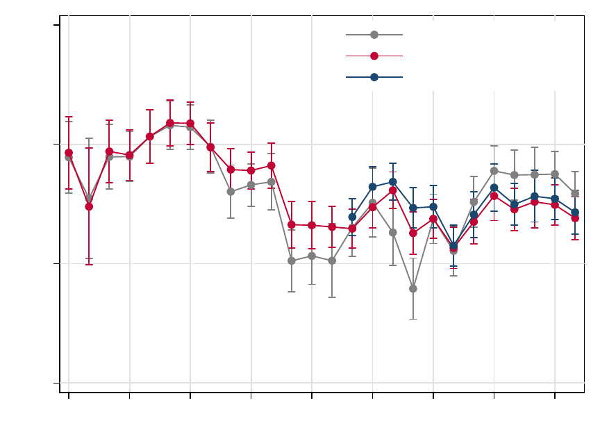
.5 .6 .7 .8

Marginal Effect

1990 1993 1996 1999 2002 2005 2008 2011 2014

Not Controlling for 2nd Liens

Controlling for 2nd Liens

Only 1st Liens

Figure A.1. Comparison of Author-Identified First Liens and those Identified by HMDA

Note: This graph plots coeﬃcients from regressions of individual loan amounts on income and covariates

from HMDA data. The blue line plots the coeﬃcients only using ﬁrst liens as identiﬁed by HMDA. The

grey line does not make any correction for second liens. The red line uses the authors’ algorithm to identify

second liens back to 1990, and corrects the loan amount to account for both mortgages.

Source: HMDA.

Ordinary Least Squares

Income Coefﬁcients Expected Mortgage Amounts Income Coefﬁencients

No CBSA-Year Fixed Effects No CBSA-Year Fixed Effects With CBSA-Year Fixed Effects

.6 .65 .7 .75 .8 .85 .9

Effects on Linear Prediction

1990 1995 2000 2005 2010 2015

11.25 11.5 11.75 12 12.25

Linear Prediction

1990 1995 2000 2005 2010 2015

.6 .65 .7 .75 .8 .85 .9

Effects on Linear Prediction

1990 1995 2000 2005 2010 2015

Using Tract-Level Census Income as an IV for Individual-Level HMDA Income

Income Coefﬁcients Expected Mortgage Amounts Income Coefﬁcients

No CBSA-Year Fixed Effects No CBSA-Year Fixed Effects With CBSA-Year Fixed Effects

.9 1 1.1 1.2 1.3 1.4

Effects on Linear Prediction

1990 1995 2000 2005 2010 2015

11.25 11.5 11.75 12 12.25

Effects on Linear Prediction

1990 1995 2000 2005 2010 2015

.9 1 1.1 1.2 1.3 1.4

Effects on Linear Prediction

1990 1995 2000 2005 2010 2015

Figure A.2. Canonical Regression using Individual-Level HMDA Mortgage Balances and Income Levels

Note: These panels graph income coeﬃcients (and 95 percent conﬁdence intervals) from regressions of individual purchase-mortgage origination

amounts determined from HMDA on measures of income. The top panels use individual income as reported in HMDA. The bottom panels instrument

for HMDA income using the most recently available Census tract income from the Census and ACS. CBSA-year ﬁxed eﬀects are omitted in the ﬁrst

and second panels of each row. All speciﬁcations control for the borrower’s race and gender interacted with year. Expected mortgage amounts are

predictions, holding income constant at its average value across all years.

Source: HMDA, decennial Census, and the American Community Survey.

Baseline Results (5-percent Sample Truncation Rule, No Fixed Effects)

Income Coefﬁcients Expected Mortgage Amounts

.2 .3 .4 .5 .6 .7 .8

Effects on Linear Prediction

1985 1987 1989 1991 1993 1995 1997 1999 2001 2003 2005 2007 2009 2011 2013

AHS Survey Year

10.5 11 11.5 12

Linear Prediction

1985 1987 1989 1991 1993 1995 1997 1999 2001 2003 2005 2007 2009 2011 2013

AHS Survey Year

Baseline Sample with Region-Year Fixed Effects

Income Coefﬁcients Expected Mortgage Amounts

.2 .3 .4 .5 .6 .7 .8

Effects on Linear Prediction

1985 1987 1989 1991 1993 1995 1997 1999 2001 2003 2005 2007 2009 2011 2013

AHS Survey Year

10.5 11 11.5 12 12.5

Linear Prediction

1985 1987 1989 1991 1993 1995 1997 1999 2001 2003 2005 2007 2009 2011 2013

AHS Survey Year

REGION=1

REGION=2

REGION=3

REGION=4

Additional Checks for Income Coefﬁcients

No 5-percent Truncation Rule With Truncation, Quantile Regression

.2 .3 .4 .5 .6 .7 .8

Effects on Linear Prediction

1985 1987 1989 1991 1993 1995 1997 1999 2001 2003 2005 2007 2009 2011 2013

AHS Survey Year

.2 .3 .4 .5 .6 .7 .8

Effects on Linear Prediction

1985 1987 1989 1991 1993 1995 1997 1999 2001 2003 2005 2007 2009 2011 2013

AHS Survey Year

Figure A.3. Robustness Checks for AHS Regressions

Note: The top row reprints the baseline AHS results from Figure 5, which are generated by a regression run

on a sample that imposes a 5-percent truncation rule for debt and income outliers. The middle row adds

ﬁxed eﬀects that are generated by interacting Census region and year. The bottom row displays income

coeﬃcients from a regression that uses a non-truncated sample (left panel) and from a quantile regression

that uses the baseline truncated sample (right panel).

Source: AHS.