Wireless Communications with
Matlab and Simulink: IEEE802.16
(WiMax) Physical Layer
by
Roberto Cristi
Professor
Dept of Electrical and Computer Engineering
Naval Postgraduate School
Monterey, CA 93943
August 2009
Table of Content:
1. Introduction: WiMax, Matlab and Simulink
2. Introduction to Digital Signal Processing and Matlab
2.1 Discrete time Signals and Systems
2.2 Fast Fourier Transform (FFT) and its Inverse (IFFT)
2.3 Convolution and Correlation
Lab 1: Matlab/Simulink Code
3. Digital Communications Fundamentals
3.1 General Structure of a Digital Communication System
3.2 Channel Losses and Noise
3.3 Complex Baseband Representation
3.4 Bit Error Probabilities
3.5 Simulink Implementation
Lab 2: Matlab/Simulink Code
4. Channel Models
4.1 Introduction and Channel Losses
4.2 Models of Fading Channels
4.3 Channel Parameterization
4.4 Estimation of Channel Parameters from Data
Lab 3: Matlab/Simulink Code
5. Multi Carrier Modulation and OFDM
5.1 Single Carrier and Multi Carrier Modulation
5.2 Orthogonal Frequency Division Multiplexing (OFDM)
5.3 Example: basics of IEEE 802.11a (WiFi)
Lab 4: Matlab/Simulink Code
6. Error Correction Coding
6.1 Channel Capacity and Error Correction Coding
6.2 Block Codes
6.3 Convolutional Codes
6.4 Code Shortening and Puncturing
6.5 Simulink Implementation of IEEE802.16 coding schemes
Simulink/Matlab Code: Error Correction
7. IEEE802.16 Implementation
7.1 Time Synchronization and Channel Estimation using the
Preamble
7.2 Channel Tracking for Mobile Applications
7.3 Simulink Implementation of IEEE802.16-2004 (Fixed)
7.4 Simulink Implementation of IEEE802.16e-2005 (Mobile)
Simulink/Matlab Code: IEEE802.16 Implementation
8. Multi Antennas
8.1 Receive Diversity
8.2 Transmit Diversity
8.3 Space Time Coding
8.4 Transmit Diversity with Space Coding in IEEE802.16
9. Issues in OFDM Systems Implementations
9.1 Peak to Average Power Ratio (PAPR)
9.2 IQ Imbalance
9.3 Frequency Offset

Introduction to IEEE 802.16 and WiMax
Existing “Area Networks” for wireless communications:
• Personal (PAN), up to a few meters. It requires simple “thumb like” transmitters
receivers. Typical: Bluetooth.
• Local (LAN), up to 300m. It requires simple “box like” devices. Typical: WiFi
(IEEE802.11)
• Wide (WAN), up to a few miles. It requires towers and cellular technology. Typical: W-
CDMA, CDMA 2000, UMTS …
IEEE 802.16 (WiMax) are possible future technologies for WAN.

• IEEE802.16 is a standard for Broadband Wireless Access (BWA) Air Interface. It is
purely technical (not commercial);
•“The WiMAX Forum®
is an industry-led, not-for-profit organization formed to certify
and promote the compatibility and interoperability of broadband wireless products
based upon the harmonized IEEE 802.16/ETSI HiperMAN standard. A WiMAX Forum
goal is to accelerate the introduction of these systems into the marketplace. WiMAX
Forum Certified™ products are fully interoperable and support broadband fixed,
portable and mobile services. Along these lines, the WiMAX Forum works closely with
service providers and regulators to ensure that WiMAX Forum Certified systems meet
customer and government requirements” (from the WiMax website
www.wimaxforum.org)
IEEE 802.16 and WiMax

Current WAN Technologies for Voice and Data
3G: CDMA2000 and UMTS. All based on Spread Spectrum
3.5G: increased capacity by combining CDMA with TDM (Time Division Multiplexing).
Voice and Data on separate channels. Current technology;
4G : to provide voice, data, multimedia services at low cost on an all IP (packets)
network. IEEE802.16 (WiMax) is one of the technologies considered.
TODAY: voice and data on separate networks;
TOMORROW: voice and data on the same network. Data using Voice Over IP
(VoIP). Advantages: flexibility, control of QoS, scalable.

Evolution of IEEE802.16:
SC, 256OFDM,
128, 512,
1024, 2048
OFDMA
Fixed, Mobile,
NOLOS
2-6GHzDec 2005802.16e-2005
SC, 256
OFDM, 2048
OFDMA
Fixed, NOLOS2-11GHzJune 2004802.16-2004
Single CarrierFixed, LOS 10-66GHzDec 2001802.16
In addition, IEEE802.16-2004 and 2005 have options based on Multi Antennas
techniques.

Introduction to Simulink
• Matlab based
• Both Continuous Time and Discrete Time Simulation
• Based on Blocksets
• Model Based Design: a software model of the environment can be
developed and the design can be tested by simulation
• Transition between “ideal” algorithms (infinite precision, floating point) to
“real world” algorithms (finite precision, fixed point);
• Automatic Code Generation: once the design is tested and validated, real
time code can be automatically generated for the target platform
• Continuous Test and Verification

Advantages (from the MathWorks slide)
Innovation
• Rapid design iterations
• “What-if” studies
• Unique features and differentiators
Quality
• Reduce design errors
• Minimize hand coding errors
• Unambiguous communication internally and externally
Cost
• Reduce expensive physical prototypes
• Reduce re-work
• Reduce testing
Time-to-market
• Get it right the first time

Simulink
• Hierarchical block
diagram design and
simulation tool
– Built-in notions of time
and concurrency
• Digital, analog/mixed
signal and event driven
• Visualize Signals
• Co-develop with C code
• Integrated with
MATLAB

Example
Wireless
Channel
TX RX
Digital
Mod
Digital
Dem
•Design
•Test
• Automatically Generate Code
… 00010101011101010100101111
0010101010010010101001001001….
Simulink Model

Modulator Demodulator
Fading
channel
Compute Errors
Display signals

Simulink has a very rich library of blocksets:

1. Introduction to Digital Signal Processing and Matlab
1. Discrete time Signals and Systems
2. Fast Fourier Transform (FFT) and its Inverse (IFFT)
3. Convolution and Correlation

1. Discrete Time Signals
1. Continuous Time to Discrete Time
2. Fundamental Signals: Delta Function, Sinusoid,
Complex Exponential

Continuous Time and Discrete Time Signals
)(tx
(
)
[]
s
xn x nT=
ss
TF /1
=
t
s
nT
[]xn
Sampling
s
F
s
T
Sampling frequency (Hz=1/sec)
Sampling interval (sec)

Fundamental Discrete Time Signals
1. “Delta” or “Impulse”
][n
δ
n
2. Sinusoid
(
)
(
)
αωαπ
+=+=
=
nAtFAnx
s
nTt
00
cos2cos][
amplitude
phase
Frequency (Hz)
Digital
Frequency
(radians)
s
F
F
0
0
2
πω
=

Generate it in matlab: plot_a_sinusoid.m
n=0:100;
A=10;
w0=2*pi/5;
alpha=0.1;
x=A*cos(w0*n+alpha);
plot(x);
Example:
kHzF
kHzF
s
10
2
0
=
=
0
2,000 2
2
10,000 5
Hz
rad
Hz
π
ωπ
==
⇒
n=[0,1,2,…,100]
x=[10*cos(0.1), … , 10*cos((2*pi/5)*100+0.1)]
(
)
(
)
0
[ ] 10cos 4,000 0.1 10cos 0.1
s
tnT
xn t n
πω
=
=+=+
10
s
FkHz=
Digital frequency:

3. Complex Exponentials
()
(
)
44344214434421
PartImaginary
0
Part Real
0
)sin()cos(
][
00
αωαω
ω
α
αω
+++=
==
+
nAjnA
eAeAeny
nj
j
nj
where imaginary basis
1−=j
Then a sinusoid becomes the “real part” of a complex signal
()
{
}
αω
αω
+
=+
nj
AenA
0
Re)cos(
0

Sinusoids and Frequency Spectrum
Complex exponentials are the “building blocks” of signals and systems.
Reasons: all operations of interest boil down to multiplications or divisions
A sinusoid in terms of complex exponentials can also be written as
() ()
00
0
cos( )
22
jn jn
AA
An e e
ω
αωα
ωα
+
−+
+= +
0
ω
0
ω
−
with two frequencies:
positive and negative

The Fast Fourier Transform (FFT) and its Inverse (IFFT)
1. Definitions
2. Examples
3. Computation in Matlab
4. Symmetry

The Fast Fourier Transform (FFT)
Given a finite sequence of data
1,...,0],[
−
=
Nnnx
x
n
0
1N
−
1. Define the FFT
{
}
xFFTX
=
∑
−
=
−
=
1
0
2
][][
N
n
n
N
jk
enxkX
π
1,...,0
−
=
Nk
where
2. … and the IFFT (Inverse FFT)
{
}
x
IFFT X=
2
1
0
1
[] []
N
j
kn
N
k
xn Xke
N
π
−
=
=
∑
0,..., 1nN=−
where
Meaning:
1,...,0],[
−
=
NkkX
is the component of the spectrum due to frequency
N
F
kF
s
=
sampling frequency
data length
Example:
|][| kX
k
10230
220
kHzF
s
10=
Let
1024N =
kHzkHzF 15.2
1024
10
220 ==

Example: example_of_fft.m
Data length N=1024;
Sampling Frequency Fs=10kHz
X=fft(x);
k=0:1023; f=k*Fs/N; % frequency axis
plot(f,abs(X))
0 1000 2000 3000 4000 5000 6000 7000 8000 9000 10000
0
500
1000
1500
2000
2500
3000
3500
4000
FFT of cosine
Hz
Freq. = 1kHz
This corresponds to the
“negative frequency”
(disregard)

Convolution and Correlation
1. Convolution as system response
2. Autocorrelation of data
3. Crosscorrelation between data sets
4. Estimation of Impulse Response using Crosscorrelation

Operations of Interest
1. Convolution. To compute the output of a Linear Time Invariant system
][nh
[]xn []
y
n
Input
signal
output
signal
Impulse
response
Definition of Convolution:
∑
+∞
−∞=
−==
l
ll ][][][*][][ nxhnxnhny
In general you deal with sequences of finite length
0
x
0
h
Input data
Impulse
response
*
convolution
=
0
y
=
Output data
]1[]1[...]2[]2[]1[]1[][]0[][
+
−
−
+
+
−
+
−
+= MnxMhnxhnxhnxhny
1
−
N
1
−
M
2
−
+
MN

In matlab:
Let
1. h be the vector of impulse response;
2. x be the input vector
Then the output vector
y=conv(h,x);
Example: convolution_of_finite_sequences.m
h=[1,0,0,0.5,0,-0.2,0,0.1]; % impulse response
n=0:200; x=2*cos(0.1*pi*n); % input signal
y=conv(h,x); % output signal
plot(y)
2. Auto Correlation.
For a signal with zero mean, to see if the samples are “correlated” with each other
Definition of Auto Correlation:
∑
+∞
−∞=
−=
n
x
mnxnxmr ][][][
*
Again, you deal with signals of finite length
1,...,0],[
−
=
Nnnx
,][][
1
][
1
0
*
∑
−
=
−=
N
n
x
mnxnx
N
mr
Example: White Noise with standard deviation
⎪
⎩
⎪
⎨
⎧
≈
==
=
∑
−
=
otherwise ,0
0 if ,|][|
1
][
1
0
22
mnx
N
mr
N
n
x
x
σ
m
][mr
x
1,...,1
−
+
−
=
NNm
x
σ

Example: xcorr_of_white_noise.m
% data
sigx=sqrt(2)
x=sigx*randn(1,1000);
plot(x);
% autocorrelation
N=length(x);
rx=xcorr(x)/N;
max_lag=length(x)-1;
m=-max_lag:max_lag;
plot(m,rx)
0 100 200 300 400 500 600 700 800 900 1000
-4
-3
-2
-1
0
1
2
3
4
white noise sequence
-1000 -800 -600 -400 -200 0 200 400 600 800 1000
-0.2
0
0.2
0.4
0.6
0.8
1
1.2
1.4
1.6
1.8
time lag
autocorrelation of x

2. Cross Correlation.
To see if two signals are “correlated” with each other
∑
+∞
−∞=
−=
n
yx
mnxnymr ][][][
*
With finite length signals:
1,...,0],[
1,...,0],[
−=
−
=
Mnny
Nnnx
1),max(,...,1),max(,][][
1
][
1
0
*
−+−=−=
∑
−
=
MNMNmmnxny
M
mr
M
n
yx

][nx []
y
n
][nh
Case of Interest: estimation of the impulse response of a Linear Time Invariant system
from input-output data
If is white noise, then
][nx
]0[/][][
xyx
rnrnh
=

Example: impulse_response_with_xcorr.m
-1.5 -1 -0.5 0 0.5 1 1.5
x 10
4
-0.5
0
0.5
1
1.5
2
2.5
-40 -20 0 20 40 60
-0.5
0
0.5
1
1.5
2
2.5
zoom in
h=[1, 0, 0.2, -0.5, 2, -0.1]; % impulse response
y=conv(h,x);
ryx=xcorr(y,x) /length(y)
h_est=ryx/ryx(length(x));

Lab 1: Introduction to DSP and Matlab
1. Generate a sinusoidal signal of a given frequency
2. Check its frequency spectrum
A. Sinusoids and the FFT:
B. White Noise, Convolution, Correlation:
1. Generate a white noise signal with a given covariance
2. Determine the output of a given Linear Time Invariant System
3. From the input-output data, estimate the impulse response of the system

A. Sinusoids and the FFT:
A.1 Generate a sinusoid with the following parameters and plot it vs time:
Amplitude
Frequency
Sampling Frequency
Phase
Length
0.5
=
A
kHzF 0.5
0
=
kHzF
S
0.15
=
0
30=
α
samples 128
plot_a_sinusoid.mReference:

A.2 Take the FFT of the sinusoid you generated, plot its magnitude (absolute value),
and verify that you obtain the frequency you expect.
Reference: example_of_fft.m

B. White Noise, Convolution, Correlation:
1. Generate a gaussian white noise signal with the following parameters:
Standard Deviation
Length
5
=
x
σ
points data 000,10
=
N
Plot its autocorrelation and verify that it is as expected.
2. This signal is the input to a system with impulse response
]3.0,0,0,0,5.0,2,0,1[
−
=h
Determine the output sequence and verify that the crosscorrelation between
input and output is a good estimate of the impulse response of the system.
Reference: impulse_response_with_xcorr.m

2. Digital Communications Fundamentals and the
Additive White Gaussian Noise (AWGN) Channel
1. General Structure of a Digital Communication System
2. Channel Losses and Noise
3. Complex Baseband Representation
4. Bit Error Probabilities
5. Simulink Implementation
References:
J. Proakis, M. Salehi, “Digital Communications,” Prentice
Hall, 2007

1. General Structure of a Digital Communications System
1.1 General Overview
1.2 Goals
1.3 Parameters of Interest

1.1 General Overview
Digital
Mod
source of
information
channel
decision
destination
noise,
disturbances,
other users
..01010110…
I
..01010010…
Errors!
bits symbols
Discrete Time
Continuous
Time
Discrete Time
symbols bits
I
Q
I
Q
Q
I
Q
Carrier
frequency
Carrier
frequency
Digital
Dem
pulses pulses
TX RX

1.2 Goals
channel
..01010110…
..01010010…
Errors!
TX RX
• Bit Error Rate within acceptable values;
• Stay within the available resources:
Transmitted
Power
Channel
Bandwidth
Noise
Interference
Variability
…
Receiver
Complexity

1.3 Parameters
RF
channel
Digital
Modulator
DAC
Digital
Demodulator
][nx
I
DAC
][nx
Q
RF
ADC
ADC
][ny
I
][ny
Q
symbols
][na
bits
symbols
][
ˆ
na
bits
)(tw
symbol
bits
N
b
=
sec
symbols
F
S
=
symbol
Joules
E
S
=
WattsFEP
SST
=
WattsP
W
=
WattsPAP
TR
×
=
W
R
P
P
SNR =
T
R
P
P
A =
Bit Error
Rate
)(tx
I
)(tx
Q
)(ty
I
)(ty
Q
pulses
pulses

I (Re)
Q (Im)
BPSK
1
+
1
−
I
Q
1
+
1
−
4-QAM
(QPSK)
→
0
b
0
1
0
1
→
0
b
0
1
→
1
b
][
0
b
],[
10
bb
Bits to Symbols:
the Constellation Mapping in 802.16 (Gray Code)
bit/symbol 1=
b
N
lbits/symbo 2=
b
N

I
Q
16-QAM
11
→
23
,bb
],,,[
3210
bbbb
10
00 01
→
01
,bb
01
00
10
11
Notice : only one bit difference between close neighbors
lbits/symbo 4=
b
N

Symbols to Pulses:
Digital to Analog (DAC) and Analog to Digital (ADC) Conversion
n
][nx
DAC
)(tg
T
)(tx
symbol
pulse
n
][ny
ADC
)(tg
R
)(ty
symbol
pulse
)(][
S
nTtgnx
−
S
nT
t
t
t
S
nT
t
∑
+∞
−∞=
−
n
S
nTtgnx )(][

Bandwidth, Symbol Rate and Transmitted Power
)(tg
(sec)t
S
T
Symbol
interval
)(HzF
SS
TF /1=
B
)(FG
Bandwidth
Symbol Rate
Energy per symbol
∫∫
+∞
∞−
+∞
∞−
== dFFGdttgE
S
22
|)(||)(|
Transmitted Power
SS
S
S
T
FE
T
E
P ×==

-4 -3 -2 -1 0 1 2 3 4
-0.4
-0.2
0
0.2
0.4
0.6
0.8
1
t
a=0.0
a=0.3
a=0.6
-1.5 -1 -0.5 0 0.5 1 1.5
0
0.5
1
1.5
f
a=0.0
a=0.3
a=0.6
()gt
Typical: Raised Cosine
• smaller bandwidth
• more ISI
• larger bandwidth
• less ISI
)(FG
110 ≤=−≤
α
S
F
B
S
F
F

2. Channel Losses and Noise
2.1 Transmitted Pulses to Received Pulses
2.2 Energy per Symbol, Power Spectral Density
2.3 Signal to Noise Ratio and “Eb/N0”

Transmit Receive
• attenuation: free space, obstacles, foliage …
•
noise: thermal, interferences from other systems/users
•
multipath: reflections from buildings, structures, hills …
•
doppler shift: motion of transmitter, receivers, reflectors …
2.1 Transmitted Pulses to Received Pulses:

Channel Attenuation
channel
)(tw
WattsBNP
W
×
=
0
WattsPAP
TR
×=
T
R
P
P
A =
WattsFEP
SST
=
Transmitted Power
Received Power
Channel Losses and Noise
Noise
F
Noise Power
Spectral Density
2
0
N
B
B

BN
FE
SNR
SS
×
×
==
0
Power Noise
Power Signal
Energy per symbol
Symbol Rate
Noise Power Spectral Density
Bandwidth
2.2 Energy per Symbol and Power Spectral Density

Thermal Noise
• Present in all electronic systems, it is dependent on temperature;
• It is “white”, in the sense that it is equally spread in frequency.
)(HzF
Power Spectral Density
2/
0
N
TKJkTN ××==
−
)/10383.1(
23
0
temperature in kelvin
Boltzman’s constant
Ambient temperature =290K
HzdBmN
dB
/174
0
−
=
In dBm:

Example:
• Temperature = 290K (ambient)
• Bandwidth = 2.0MHz
Noise Power =
()
dBmHzdBmBN
dB
111102log10/174
6
100
−=×+−=

⎟
⎟
⎠
⎞
⎜
⎜
⎝
⎛
⎟
⎠
⎞
⎜
⎝
⎛
=
⎟
⎟
⎠
⎞
⎜
⎜
⎝
⎛
⎟
⎠
⎞
⎜
⎝
⎛
=
00
N
E
B
F
N
N
E
B
F
SNR
bS
b
SS
symbolper bits
(Joules)bit per Energy
(Joules) symbolper Energy
density spectralpower noise
sec)/1(bandwidth
(1/sec) rate symbol
0
=
=
=
=
≥==
=
b
b
S
S
S
N
E
E
N
FHzB
F
2.3 Signal to Noise Ratio and “Eb/N0”

3. Complex Baseband Representation
3.1 Complex Signals
3.2 Baseband Channel Representation

3.1 Complex Signals
][nx
I
][nx
Q
DAC
)(tg
T
(
)
tFA
c
π
2cos
DAC
)(tg
T
(
)
tFA
c
π
2sin
−
)(ty
T
][ny
I
][ny
Q
)(tg
R
(
)
tFA
c
π
2cos
)(tg
R
()
tFA
c
π
2sin
−
channel
s
T
)(ty
R
)(tx
I
)(tx
Q
)(ty
I
)(ty
Q
I
Q
I
Q
Received
Transmitted
Symbols:

Recall: Complex Numbers and Complex Exponentials
4342143421
)sin()cos(
αα
α
AjAAe
j
+=
amplitude phase (angle)
Real Part Imaginary Part
1−=j
A
α
Re
Im
As a consequence:
)2sin()2cos(
2
tFjAtFAAe
CC
tFj
C
ππ
π
+=

It is easier to define one complex signal which combines In Phase and
Quadrature components:
][][][ njxnxnx
QI
+=
DAC
)(tg
T
tFj
c
Ae
π
2
)(ty
T
)(tg
R
channel
s
T
)(ty
R
Re{.}
tFj
c
Ae
π
2−
][][][ njynyny
QI
+=
Re
Im
Re
Im

If the carrier frequency is larger than the bandwidth of the filters, then it
can be simplified as
][][][ njxnxnx
QI
+=
DAC
)(tg
T
tFj
c
e
A
π
2
2
)(tg
R
channel
s
T
tFj
c
e
A
π
2
2
−
][][][ njynyny
QI
+=
Baseband Channel
Re
Re
Im

)(tg
T
tFj
c
e
A
π
2
2
)(tg
R
tFj
c
e
A
π
2
2
−
3.2 Baseband Channel Representation
)(tx
)(ty
C
F
C
F−
F
Real channel
)(FC
)(tg
T
)(tg
R
)(tx
)(ty
F
Complex
Baseband
channel
)(
2
C
FFC
A
−
+
⇒
⇐
same
Advantage: all signals
at lower frequencies,
therefore much easier to
simulate and analyze.

Encoder
source of
information
Baseband
Channel
Digital
Modulator
Decoder
Digital
Demodulator
Received
Data
][nx
][ny
Digital Transmitter/Receiver with Baseband Channel:
complex
Binary Complex
Binary
Complex

4. Bit Error Probabilities for M-QAM Modulation
4.1 “Eb/N0” and SNR for MQAM Signals
4.2 Probability of Symbol Error in Additive White Gaussian
Noise (AWGN) Channel;

⎟
⎠
⎞
⎜
⎝
⎛
⎟
⎟
⎠
⎞
⎜
⎜
⎝
⎛
==
B
F
N
EM
BN
TE
SNR
SbSS
0
2
0
)(log/
Energy per bit
# of bits per symbol
M-QAM:
4.1 “Eb/N0” and SNR for MQAM Signals
….01001011001010…
M-QAM

SNR
MN
E
b
⎟
⎟
⎠
⎞
⎜
⎜
⎝
⎛
=
)(log
1
20
Therefore, if :
BF
S
≅
Significance: the error probabilities for MQAM are functions of
0
/ NE
b

Example.
Given:
Transmitted Power: 100mW
Bandwidth: 1.75MHz
Channel Attenuation: -120dB
Modulation: QPSK (2 bits/symbol)
Compute
:
0
/ NE
b
Assume: Thermal Noise only at ambient temperature

Solution:
1. Energy per Symbol at the transmitter
HzdBmHzmWMHzmWE
S
/4.42/1014.5775.1/100
6
−=×==
−
2. Energy per Symbols at the receiver
HzdBmE
S
/4.1621204.42
−
=
−−=
3. SNR at the receiver
dB
N
E
SNR
dB
S
6.11)174(4.162
0
=−−−=
⎟
⎟
⎠
⎞
⎜
⎜
⎝
⎛
=
4. Finally
()
dBNE
dB
b
6.82log106.11/
100
=
−
=

4.2 Probability of Symbol Error in AWGN
BPSK:
(
)
0
2
N
E
S
b
QP =
4-QAM:
M-QAM:
(
)
0
22
N
E
S
b
QP ≈
⎟
⎟
⎠
⎞
⎜
⎜
⎝
⎛
⎟
⎟
⎠
⎞
⎜
⎜
⎝
⎛
⎟
⎠
⎞
⎜
⎝
⎛
−
≈
0
2
1
log3
4
N
E
M
M
QP
b
S
Probability of Bit Error with Gray Coding:
M-QAM:
Sb
P
M
P
)(log
1
2
≈
where
⎟
⎠
⎞
⎜
⎝
⎛
=
=
∫
+∞
−
2
2
1
)(
2
1
2
x
erfc
exQ
x
dtt
π

Symbol Error Rates (Exact Values)
-5 0 5 10 15 20
10
-6
10
-5
10
-4
10
-3
10
-2
10
-1
Symbol Error Rate
Eb/No dB
Prob. bit Error
4QAM
BPSK
16QAM
64QAM

Example.
Same as previous example
Compute
: a. Symbol Error Rate, b. Bit Error Rate
Solution:
1. From the previous Example
dBNE
b
6.8/
0
=
2. Symbol Error Rate: errors per symbol (see graphs)
4
10
−
3. Bit Error Rate: errors per bit
54
1052/10
−−
×=

5. Simulink Implementation
5.1 Fundamentals of Simulink
5.2 Digital Communications in AWGN: Simulink Implementation;
5.3 Example

5.1 Fundamentals of Simulink
Simulink has three classes of blocksets:
• sources (outputs only)
• processes (inputs/outputs)
• sinks (inputs only)
source
process
sink
• generate data
• read data
•import files …
• display results
• plots, scopes…
• send data to devices

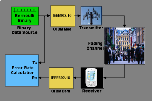
5.2 Digital Communications in AWGN: Simulink Implementation
Generate Complex Data
BaseBand
Channel
Display Received Data
Compute Bit
Error Rate
Simulink Model: AWGN_no_coding.mdl

5.3 Example
M=4; % MQAM modulation
Fs=10^6; % symbol rate (1/sec)
SNRdB=20; % SNR in dB’s
PT=5; % Transmitted Power in Watts
A=1/100; % Channel Attenuation
PR=A*PT; % Received Power
Let’s simulate a Digital Communications System with the
following parameters:

Edit > Model Properties
Enter the parameters

Generate Complex Data
• M-QAM
• Fs symbols/sec
Communications Sources
>Random Data Sources
>>
Bernoulli Binary
Modulation
>Digital Baseband Mod
>>AM
>>>
Rectangular QAM
Parameters:

Baseband Channel
⎟
⎟
⎠
⎞
⎜
⎜
⎝
⎛
+×= ][][
1
][ nw
SNR
P
nxPA
P
ny
T
T
R
Transmitter Gain
Channels
> AWGN Channel

Analysis of Data by Computer Simulation
Blocks:
• Comms Sinks > Error Rates Calculation
•Simulink > Sinks > Display
error rate
errors
bits
received
transmitted

Lab2: Digital Communications Fundamentals
M=4; % MQAM modulation
Fs=10^6; % symbol rate (1/sec)
PT=2; % Transmitted Power in Watts
A=1/50; % Channel Attenuation
PR=A*PT; % Received Power
Given a digital Communication System defined by the following parameters:
1. Simulate the system for the following values of the Signal to Noise Ratio:
SNR=5,10,20dB
2. For each case determine the probability of bit error experimentally
3. Compare with the theoretical values
References: AWGN_no_coding.mdl
bit_error.m

Probability of Symbol Error
-5 0 5 10 15 20
10
-6
10
-5
10
-4
10
-3
10
-2
10
-1
Symbol Error Rate
Eb/No dB
Prob. bit Error
4QAM
BPSK
16QAM
64QAM
Probability of Bit Error=
Probability of Symbol Error / log2(M)

3. Channel Models
1. Introduction and Channel Losses
2. Models of Fading Channels
3. Channel Parameterization
4. Estimation of Channel Parameters from Data

1. Introduction and Channel Losses
1.1. Large Scale fading: Free Space Losses
1.2. Medium Scale Fading: Shadowing
1.3. Small Scale Fading: Multipath
References:
A. Goldsmith, Wireless Communications, Cambridge Univ.
Press, 2005 – Chapter 2.

1. Large Scale
Fading: due to
distance and
multipath
2. Medium Scale
Fading: due to
shadowing and
obstacles
3. Small Scale
Fading: due to
multipath
Signal Losses due to three Effects:

Wireless Channel
Several Effects:
• Path Loss due to dissipation of energy: it depends on distance only
• Shadowing due to obstacles such as buildings, trees, walls. Is caused by
absorption, reflection, scattering …
• Self-Interference due to Multipath.
transm
rec
P
P
10
log10
distancelog
10
Frequencies of Interest: in the UHF (.3GHz – 3GHz) and SHF (3GHz – 30 GHz)
bands;

Line of Sight (LOS) only
Non Line of Sight (NOLOS)
Frequencies:
30GHz
3GHz
300MHz
UHF
SHF
6GHz
Line of Sight and Frequencies

Path Loss due to Free Space Propagation:
Transmit
antenna
Receive
antenna
2
4
rec transm
PP
d
λ
π
⎛⎞
=
⎜⎟
⎝⎠
wavelength
c
F
λ
=
d
Path Loss in dB:
10 10 10
10log 20log ( ( )) 20log ( ( )) 32.45
transm
rec
P
LFMHzdkm
P
⎛⎞
== ++
⎜⎟
⎝⎠
1.1. Large Scale Propagation: Free Space
For isotropic antennas:

Free Space Attenuation
10
log ( )d
distance
0
10d
0
d
decdB /20
Valid for:
• Satellite Communicationss
• Point to Point LOS Microwave
• Reference for Path Loss Models
p
L
dBL
p
20=Δ
100/20
2121 recrecpp
PPdBLL
=
⇒=−

Typical of open environments such as rural roads
T
h
R
h
T
h
R
h
T
x
R
x
l
T
x
R
x
l
1
j
e
φ
−
Δ
+
2
TR
xx
φπ
λ
+−
Δ=
l
d
• Small to medium distances
constructive/distructive interference
• Large distances
monotonic
Multipath Models: Two Ray Reflection

10
0
10
1
10
2
10
3
10
4
10
5
-220
-200
-180
-160
-140
-120
-100
-80
-60
-40
-20
d in meters
P
rec
/P
trans
in dB
f=0.3GHz
f=3GHz
f=30GHz
Two Ray Model Power Received
40 /dB dec
−
independent of
frequency
rec
trans
P
P
4
22
d
hh
P
P
RT
trans
rec
≈
Assume: reflecting surface a pure dielectric

Free Space:
Two Ray Approximation:
T
h
R
h
10
log ( )d
p
L
10
1
10
−
0
10
2
10
−
20dB
40dB
)(log20)4/(log20
1010
dL
p
+
−=
πλ
)(log40)(log20
1010
dhhL
RTp
+
−=
Compare the two:

2. Medium Scale Fading: Losses due to Buildings, Trees,
Hills, Walls …
{
}
χ
+
=
pp
LEL
The Power Loss in dB is random:
approximately gaussian with
dB126
−
≈
σ
expected value
random, zero mean

0
0
10
log10}{ L
d
d
LE
p
+
⎟
⎟
⎠
⎞
⎜
⎜
⎝
⎛
=
γ
Path loss
exponent
Reference distance
• indoor 1-10m
• outdoor 10-100m
Free space loss at reference
distance
dB
Values for Exponent :
Free Space 2
Urban 2.7-3.5
Indoors (LOS) 1.6-1.8
Indoors(NLOS) 4-6
γ
Average Loss

• Okumura: urban macrocells 1-100km, frequencies 0.15-1.5GHz,
BS antenna 30-100m high;
• Hata: similar to Okumura, but simplified
• COST 231: Hata model extended by European study to 2GHz
Empirical Models for Propagation Losses to Environment

Typical: Hata Models (1980)
Frequencies 0.15-1.5GHz
10
44.9 6.55lo
g
()h
β
=−
01010
2
010
2
010 10
69.55 26.16lo
g
( ) 13.82lo
g
() ()
2log ( /28) 5.4
4.78log ( ) 18.33log ( ) 40.94
TR
f
hah
f
ff
α
α
αα
αα
== + − −
=− −
=− + −
urban
suburban
rural
10
log ( )d
p
L
f = frequency in MHz
h
T
, h
R
= transmitter antenna elevation over average terrain (in
meters)
where
Propagation Loss
10
lo
g
()
p
L
d
α
β
=+
()
R
ah
corrective factor for receiver antenna

()
(
)
10 10
( ) 1.1log ( ) 0.7 1.56log ( ) 0.8
RR
ah f h f dB=−− −
()
2
10
( ) 3.2 log (11.75 ) 4.97
RR
ah h dB=−
Receiver antenna correcting factor
Small to medium city
Large city

COST 231 Model: Urban Model
10
44.9 6.55lo
g
()h
β
=−
01010
46.3 33.9lo
g
( ) 13.82lo
g
() ()
TR
f
hah
α
α
== + − −
where
Propagation Loss
10
log ( )
p
M
L
dC
α
β
=+ +
0 medium sized city and suburbs
3 metropolitan area
M
dB
C
dB
⎧
=
⎨
⎩
Restrictions:
1.5 2
30 200
110
120
T
R
GHz f GHz
mh m
mh m
km d km
<
<
<<
<<
<<

Example:
Base
Station
Subscriber
md 500
=
T
P
?
=
R
P

χγ
++
⎟
⎟
⎠
⎞
⎜
⎜
⎝
⎛
=
0
0
10
log10 L
d
d
L
p
Channel:
dB
dBL
md
6
3
45
1
0
0
=
=
=
=
σ
γ
Transmitted Power:
dBmWatt 300.1
=
Received Power:
χ
χ
+
−
=
+
+
×
×
−
=
−
= dBmLP
pR
96)45500log310(3030
10
Bandwidth: 10MHz
Noise:
Given:
HzdBmN /174
0
−
=
thermal
Noise at the Receiver:
dBmP
Noise
10410log10174
7
10
−=+−=
Then:
SNR at the receiver:
dBSNR
χ
χ
+=
−
−
+
−
=
8)104(96
random

Probability that the SNR is sufficiently large
()
⎟
⎠
⎞
⎜
⎝
⎛
==>
∫
+∞
⎟
⎠
⎞
⎜
⎝
⎛
−
σσπ
χ
σ
2
2
1
2
1
2
2
1
a
erfcdxeaP
a
x
Where we define
∫
+∞
−
=
x
t
dtexerfc
2
2
)(
π
()( )
⎟
⎟
⎠
⎞
⎜
⎜
⎝
⎛
−
=>+=>
62
8
2
1
8
a
erfcaPaSNRP
χ
BPSK: a=3dB 16QAM: a=14.7dB
-1 -0.5 0 0.5 1 1.5 2
0
0.1
0.2
0.3
0.4
0.5
0.6
0.7
0.8
0.9
1
(1/2)erfc(x)
x
75.0
10.0
Required for low BER:
16QAM 10% of
the time
BPSK 75% of
the time
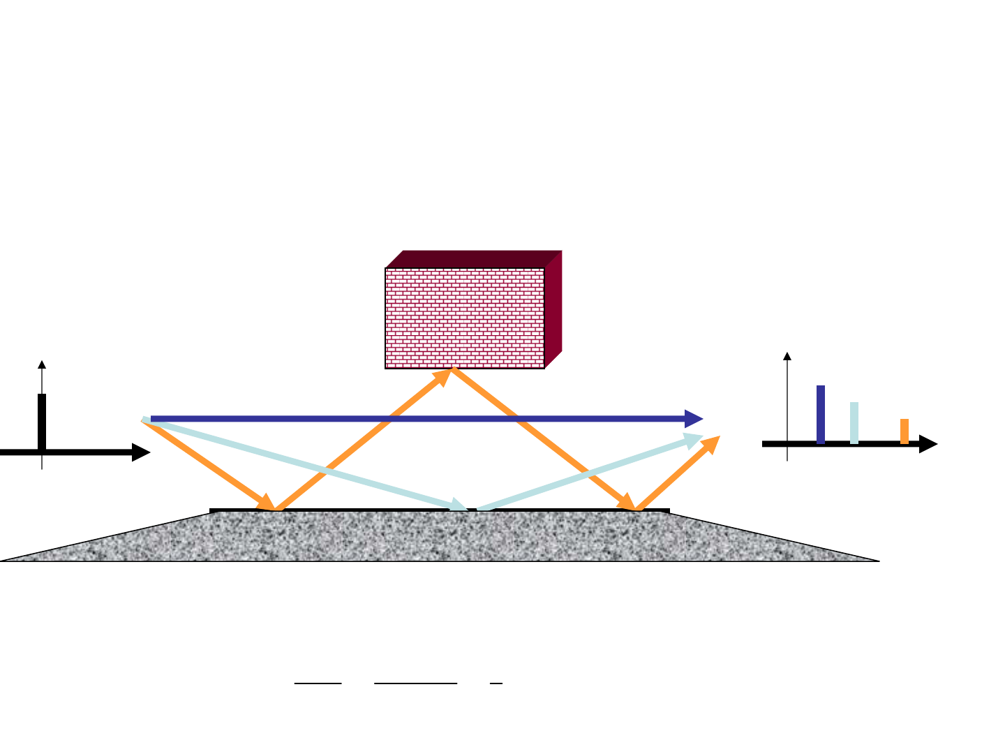
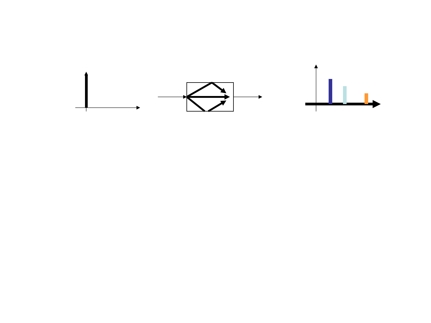
3. Small Scale Fading due to Multipath.
a. Spreading in Time: different paths have different lengths;
time
Transmit
Receive
0
() ( )
x
ttt
δ
=−
0
t
0
( ) ( ) ...
kk
yt h t t
δ
τ
=
+−−+L
1
τ
2
τ
3
τ
0
t
2
1
3
8
100 10
sec
310c
τμ
== =
×
Example for 100m path difference we have a time delay
Typical values channel time spread:
channel
0
() ( )
x
ttt
δ
=−
1
τ
2
τ
M
AX
τ
0
t
0
t
1
Indoor 10 50 sec
Suburbs 2 10 2 sec
Urban 1 3 sec
Hilly 3-10 sec
n
μ
μ
μ
−
−
×−
−

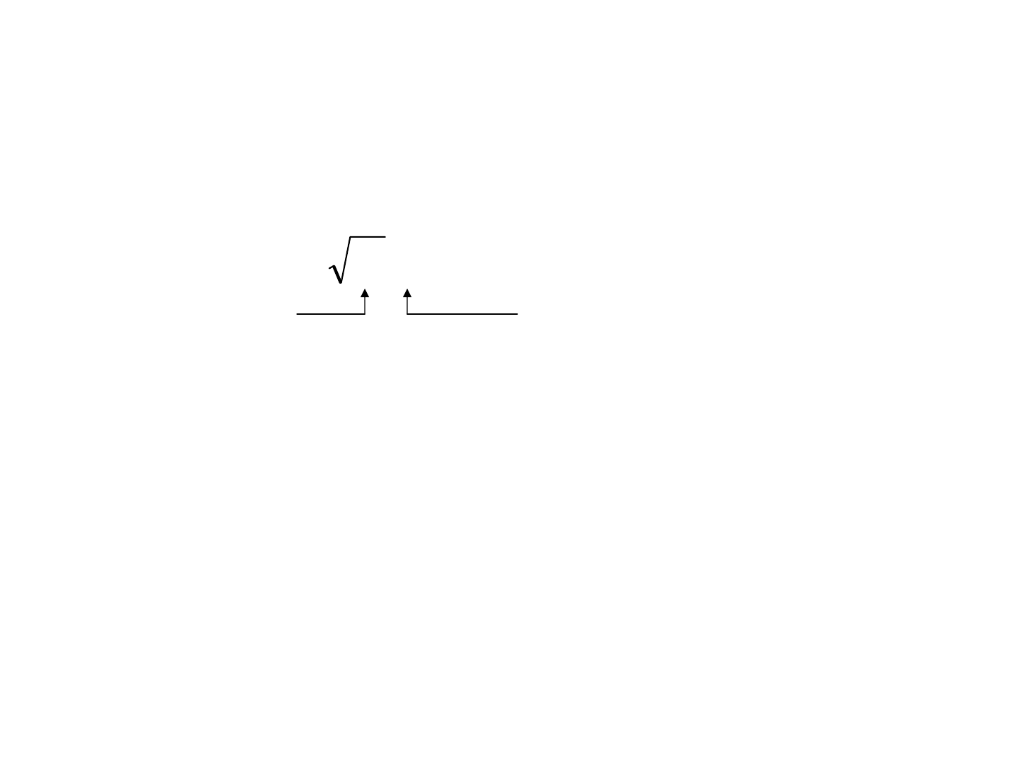
b. Spreading in Frequency: motion causes frequency shift (Doppler)
time
time
Transmit
Receive
Frequency (Hz)
Doppler Shift
v
c
f
2
()
c
j
ft
T
xt Xe
π
=
(
)
2
()
c
j
fft
R
yt Ye
π
+Δ
=
for each path
c
f
f
+
Δ
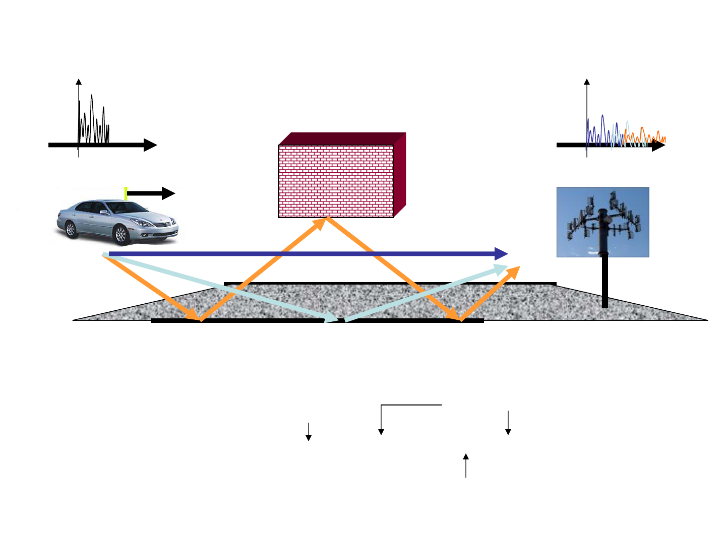
time
Transmit Receive
v
Put everything together
time
2( )( )
() Re ( )
kc k
jF tF
k
k k
yt xt ea
τπ
τ
+−Δ
⎧
⎫
=−
⎨
⎬
⎩⎭
∑
Each path has … …shift in time …
…shift in frequency …
… attenuation…
(this causes small scale time variations)
)(tx )(ty
paths

2. Models of Fading Channels
2.1. Statistical Models of Fading Channels
2.2. Non Line of Sight (Rayleigh) and Line of Sight (Rice) Channels
2.3. Simulink Example

2.1 Statistical Models of Fading Channels
Several Reflectors:
Transmit
Receive
v
()
x
t
() ()yt y t=
∑
l
l
each reflector has several
paths all with different time
delays and doppler shifts

For each path with NO Line Of Sight (NOLOS):
v
r
()yt
l
τ
l
average time delay
2( ( ))
() Re ( )
c kk
jF t
k k
F
k
yt ae xt
πτε
τ ε
+−−Δ
⎧⎫
⎛⎞
=−−
⎨⎬
⎜⎟
⎝⎠
⎩⎭
∑
l
ll
• each time delay
• each doppler shift
k
τ
ε
+
l
cos( )
k k
F
v
θ
λ
Δ =

{}
22() 2
2
() Re ( )
Re () ()cos(2 ) ()sin(2 )
kkkcc
c
jtjF jFt
k
jFt
IcQc
k
F
k
F
yt e ea xt e
rte r t Ft r t Ft
τππ π
π
τ
ππ
−+ΔΔ
⎧⎫
⎛⎞
=−
⎨⎬
⎜⎟
⎝⎠
⎩⎭
== −
∑
In Phase and Quadrature Components
(
)
2( )
2
() () () ( )
ck k
k
jFF
jFt
IQ k
k
rt r t jr t ae e xt
πτε
π
τ
−+Δ+
Δ
=+ ≅ −
∑
l
l
Assume
() ( )
k
xt xt
ε
≅
−
… leading to this:
() () ( )rt c txt
τ
=−
ll
with
(
)
2( )
2
()
ck k
k
jFF
jFt
k
k
ct ae e
π
τε
π
−+Δ+
Δ
=
∑
l
l
Some mathematical manipulation …
random, time varying

Statistical Model for the time varying coefficients
()
2cos 2( cos)
1
()
kkkc
vv
M
jtjF
k
k
ct ae e
ππτ
λλ
θθ
ε
−+ +
=
=
∑
l
l
random
random
{()} 0Ec t =
l
k
θ
since random uniformly distributed in
[0,2 ]
π
{}
2cos
*2
1
() ( ) {| |}
k
v
M
j
t
k
k
Ectc t t E a e
π θ
λ
−
Δ
=
+Δ =
∑
ll
By the CLT is gaussian with:
()ct
l
Assume
Then
2
{| | }
k
P
Ea
M
=
l
{}
2cos 2cos
*
1
1
() ( )
k
vv
M
j
t
j
t
k
Ectc t t P e PE e
M
π θπ θ
λλ
−Δ −Δ
=
⎧
⎫
+Δ = =
⎨
⎬
⎩⎭
∑
ll l l
2
2cos
0
0
1
(2 )
2
v
jt
D
P
edPJFt
π
π
λ
θ
θπ
π
−Δ
=
=Δ
∫
ll

Each coefficient is complex, gaussian, WSS with autocorrelation
{
}
*
0
() ( ) (2 )
D
Ectc t t PJ F t
π
+
Δ= Δ
ll l
()ct
l
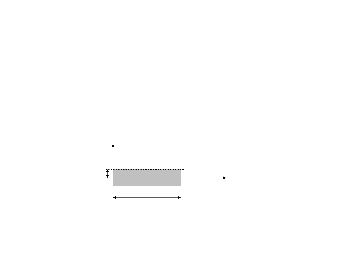
And PSD
2
21
if | |
()
1(/ )
0 otherwise
D
D
D
P
FF
F
SF
FF
π
⎧
<
⎪
=
−
⎨
⎪
⎩
l
l
with maximum Doppler frequency.
D
F
)(FS
l
D
F
F
This is called Jakes
spectrum.

Bottom Line. This:
time
v
time
)(tx )(ty
1
τ
1
()ct
τ
l
()ct
l
N
τ
()
N
ct
L
L
()yt
∑
)(tx
… can be modeled as:
delays
1
τ
τ
l
N
τ
time
time
time
For each path
)()( tgPtc
ll
=
• unit power
• time varying (from autocorrelation)
• time invariant
• from power distribution

Parameters for a Multipath Channel (No Line of Sight):
Time delays:
[
]
L
τ
τ
τ
L
21
sec
Power Attenuations:
[
]
L
PPP L
21
dB
Doppler Shift:
D
F
Hz

Non Line of Sight (NOLOS) and Line of Sight (LOS) Fading Channels
1. Rayleigh (No Line of Sight).
Specified by
:
Time delays
Power distribution
],...,,[
21 N
T
τ
τ
τ
=
],...,,[
21 N
PPPP
=
Maximum Doppler
D
F
0)}({ =tcE
l
2. Ricean (Line of Sight)
0)}({
≠
tcE
l
Same as Rayleigh, plus Ricean Factor
Power through LOS
Power through NOLOS
TotalLOS
P
K
K
P
+
=
1
TotalNOLOS
P
K
P
+
=
1
1
K

-K-
Transmitter
Gain
B-FFT
Spectrum
Scope
Rectangular
QAM
Rectangular QAM
Modulator
Baseband
-K-
Receiver
Gain
Rayleigh
Fading
Multipath Rayleigh
Fading Channel
-K-
Channel
Attenuation
Bernoulli
Binary
Bernoulli Binary
Generator
Simulink Example
Rayleigh Fading Channel
Parameters
M-QAM Modulation
Bit Rate

Set Numerical Values:
modulation
power
channel
CD
F
c
v
F =
Recall the Doppler Frequency:
carrier freq.
sec/103
8
m×
velocity
Easy to show that:
(
)
(
)()
GHz
C
hkm
Hz
D
FvF
/
≈

Typical Received Power Spectrum
-K-
Transmitter
Gain
B-FFT
Spectrum
Scope
Rectangular
QAM
Rectangular QAM
Modulator
Baseband
-K-
Receiver
Gain
Rayleigh
Fading
Multipath Rayleigh
Fading Channel
-K-
Channel
Attenuation
Bernoulli
Binary
Bernoulli Binary
Generator
2/
S
F
2/
S
F−
HzF
D
70
=
MHzF
S
10
=
MHzF
b
20
=
2 (QPSK)
Doppler freq:
Symbol rate:
Bit rate:
Bits/Symbol:

Similar Example, different parameters
-K-
Transmitter
Gain
B-FFT
Spectrum
Scope
Rectangular
QAM
Rectangular QAM
Modulator
Baseband
-K-
Receiver
Gain
Rayleigh
Fading
Multipath Rayleigh
Fading Channel
-K-
Channel
Attenuation
Bernoulli
Binary
Bernoulli Binary
Generator
2/
S
F
2/
S
F−
HzF
D
2
=
MHzF
S
10
=
MHzF
b
20
=
2 (QPSK)
Doppler freq:
Symbol rate:
Bit rate:
Bits/Symbol:

Channel Parameterization
1. Time Spread and Frequency Coherence Bandwidth
2. Flat Fading vs Frequency Selective Fading
3. Doppler Frequency Spread and Time Coherence
4. Slow Fading vs Fast Fading
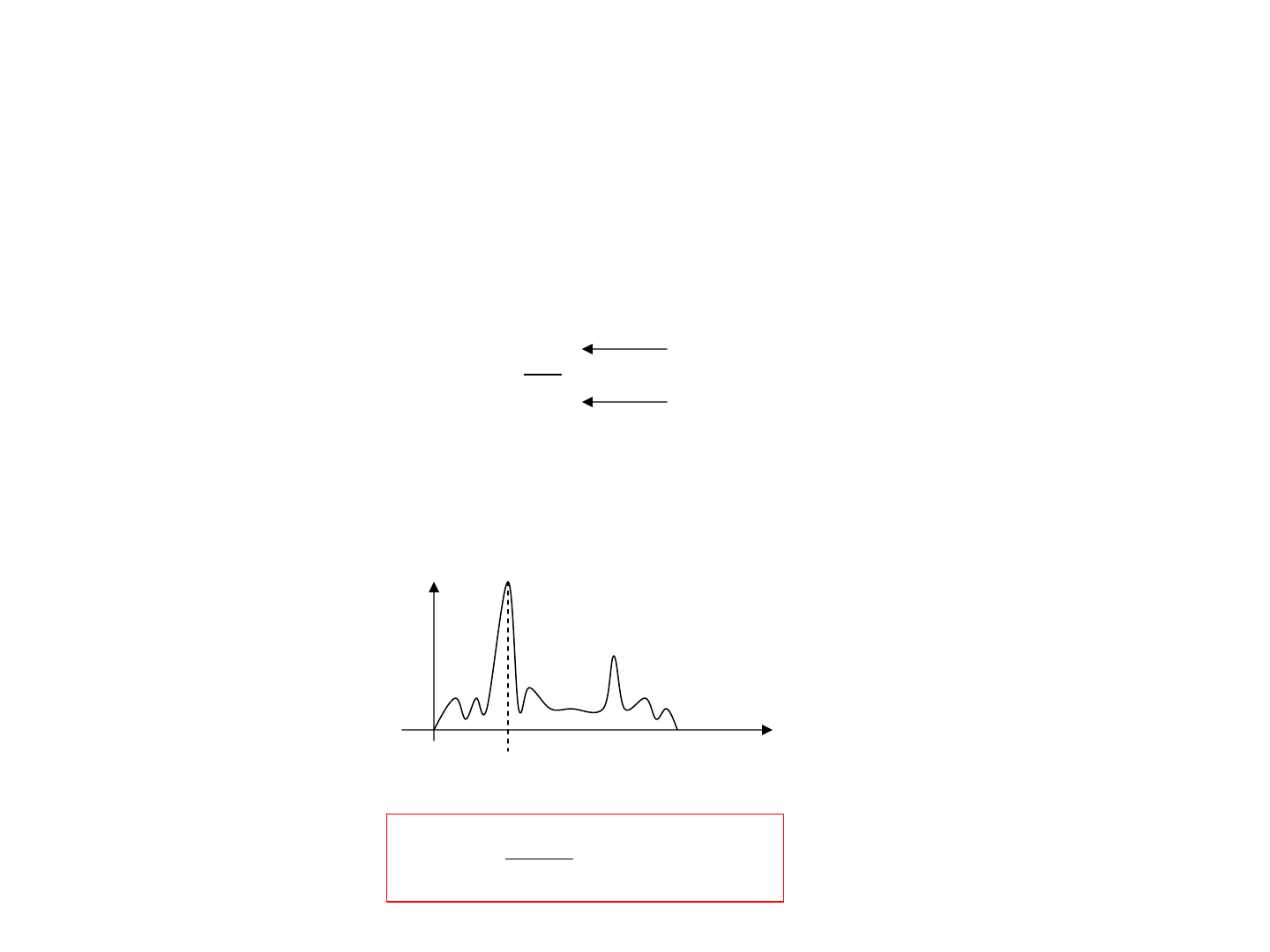
Recall that the Channel Spreads in Time (due to Multipath):
channel
0
() ( )
x
ttt
δ
=−
M
AX
τ
0
t
RMS
τ
0
10
−
20
−
Received Power
time
1
5
c
R
MS
B
τ
=
×
1. Time Spread and Frequency Coherence Bandwidth
FT
frequency
Coherence Bandwidth
Channel “Flat” up to the
Coherence Bandwidth

2. Flat Fading vs Frequency Selective Fading
• Based on Channel Time Spread:
Signal
Bandwidth
Frequency Coherence
Signal Bandwidth
<
>
Frequency Selective
Fading
Flat Fading
F
F
Frequency
coherence
Just attenuation, no distortion
Distortion!!!
F
1
5
c
R
MS
B
τ
=
×

Example: Flat Fading
Channel : Delays T=[0 10e-6 15e-6] sec
Power P=[0, -3, -8] dB
Symbol Rate Fs=10kHz
Doppler Fd=0.1Hz
Modulation QPSK
Spectrum: fairly uniform
Very low Inter Symbol
Interference (ISI)

Example: Frequency Selective Fading
Channel : Delays T=[0 10e-6 15e-6] sec
Power P=[0, -3, -8] dB
Symbol Rate Fs=1MHz
Doppler Fd=0.1Hz
Modulation QPSK
Spectrum with deep
variations
Very high ISI

3. Doppler Frequency Spread and Time Coherence
C
T
⎫
⎪
⎪
⎪
⎬
⎪
⎪
⎪
⎭
same
response
()xt ()yt
9
16
C
D
T
F
π
≈
Coherence Time:
Max Doppler
different
response
∑
=
−=
M
txtcty
1
)()()(
l
ll
τ
)()( ttctc
Δ
+
≅
ll
DC
FTt /1|| <
≤
Δ
if
4. Slow Fading vs Fast Fading
• Based on Doppler Spread Delay and Time Coherence:
Symbol
period
Time Coherence
Symbol period
<
>
Slow Fading
Fast Fading
Time
coherence
tt
Channel quickly changing
Channel almost time invariant
9
16
C
D
T
F
π
≈

Time Spread
Frequency Spread
),( FtS
F
t
RMS
τ
D
F
Summary of Time/Frequency spread of the channel
Frequency
Coherence
1
5
c
R
MS
B
τ
=
×
Time
Coherence
9
16
C
D
T
F
π
≈
mean
τ

Channel Estimation from Data
1. Recall Impulse Response Identification from
Correlation
2. Estimation of Time Spread and Doppler Shift
3. Simulink/Matlab Example
4. Stanford University Interim (SUI) Channel Models
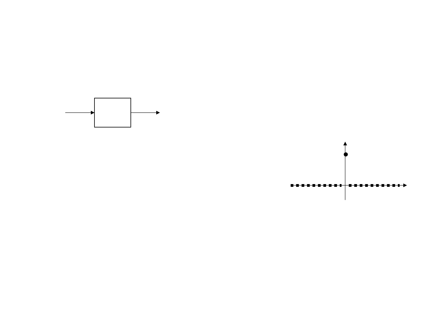
Estimation of Channel Characteristics from Input - Output data.
1. For Linear Time Invariant (LTI) systems:
][nx
][ny
][nh
∑
+∞
−∞=
−==
m
knxkhnxnhny ][][][*][][
Excite the system with white noise and unit variance
{
}
][][][][
*
mmnxnxEmR
xx
δ
=−=
m
and compute the crosscorrelation between input and output
{}
{}
][][][][][][
][][][
*
*
mhkmkhmnxknxEkh
mnxnyEmR
kk
yx
=−=−−=
−=
∑∑
∞+
−∞=
∞+
−∞=
δ

In matlab:
x
y
][nx
][ny
?
1. Get data (same length for simplicity):
2. Compute crosscorrelation between input and output:
h=xcorr(x,y);
If x[n] is white noise, h[n] is the impulse response.

2. For a Linear Time Varying Channel:
][nx
][ny
],[ nmh
∑
+∞
−∞=
−=
k
knxnkhny ][],[][
Known:
1. Sampling frequency
2. Upper bound on max Doppler Frequency
s
F
maxD
F

1. Collect Data and partition in blocks of length :
x
y
L
L
minDs
TTN
<
<×
maxD
s
F
F
N <<
xN=reshape(x,N,length(x)/N);
yN=reshape(x,N,length(y)/N);
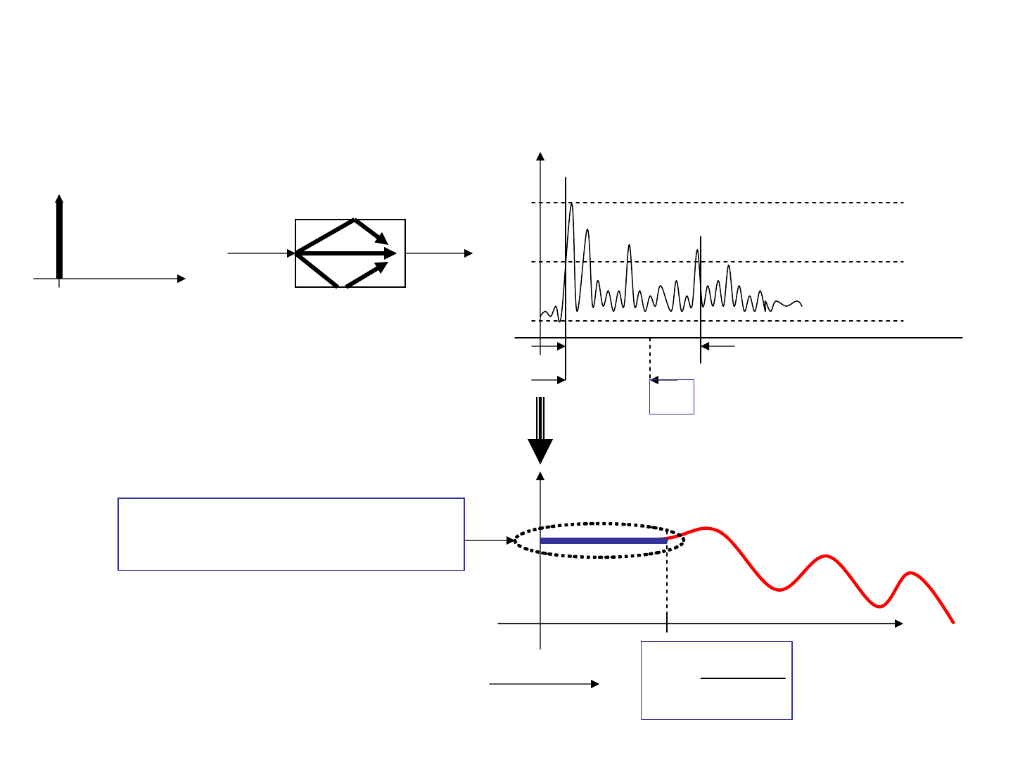
[]
L
N
xN,yN=
2. Estimate impulse response in each block
0=nNn = Nn 2
=
Nn l
=
hN=xcorr(xN,yN);
L
hN=
[
Nn
nmh
l=
],[
l
m
B
N
B
N
]
L
L
NNn
B
×
=

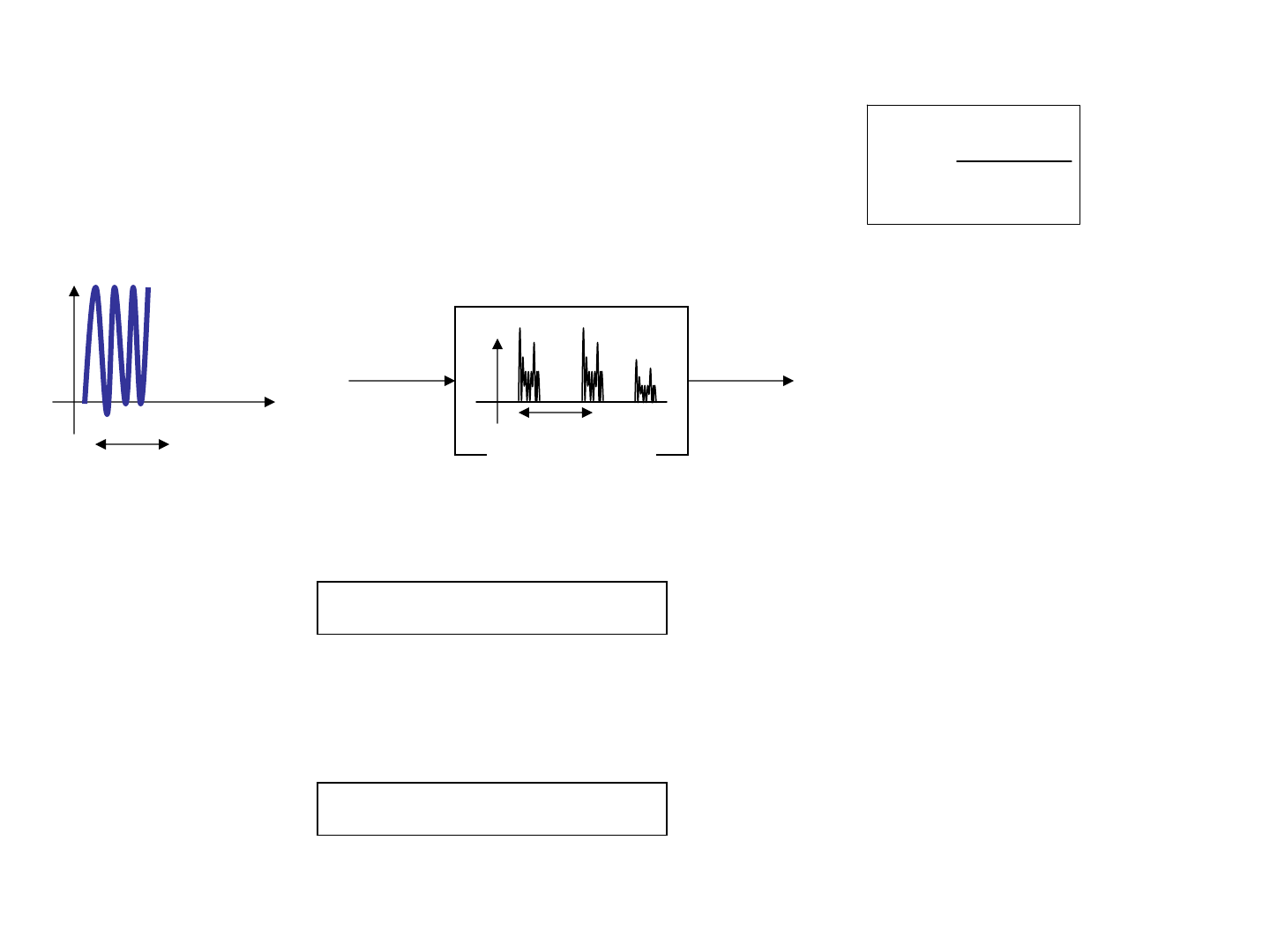
3. Compute Power Spectrum on each row, to determine time variability of the
channel (If the channel is Time Invariant all columns of hN are the same):
hN=
[
Nn
nmh
l=
],[
l
m
L
L
S=fft(hN’);
S=S’.*conj(S’);
S=
[
],[ kmS
(time) m
(freq.) k
]
]
N
B
N
⇒

4. Take the sum over rows for Doppler Spread and sum over columns for
Time Spread (fftshift each vector to have “zero” term (sec or Hz) in the
middle
s
Fmt /
=
B
s
N
NF
kf
)/(
=
St
Sf
Frequency Resolution:
Hz
NN
F
F
B
S
)length(sec data total
1
=
×
=Δ
Therefore if we want to a resolution in the doppler spread of (say) 1Hz,
we need to collect at least 1 sec of data.
Time Resolution:
S
Ft /1
=
Δ

Example: % channel
Fs=10^6; % sampling freq. In Hz
P=[0,-2,-3]; % attenuations in dB
T=[0, 10, 15]*10^(-6); % time delays in sec
fd=70; %doppler shift in Hz
y
To Workspace1
x
To Workspace
Rectangular
QAM
Rectangular QAM
Modulator
Baseband
Rayleigh
Fading
Multipath Rayleigh
Fading Channel
Bernoulli
Binary
Bernoulli Binary
Generator
test_scattering.mdl

Channel Freq. Response:

-1.5 -1 -0.5 0 0.5 1
x 10
-4
0
1
2
3
4
5
6
7
8
9
x 10
-3
Time Spread
time (sec)
-1000 -800 -600 -400 -200 0 200 400 600 800 1000
0
0.2
0.4
0.6
0.8
1
1.2
x 10
-3
Frequency Spread
frequency (Hz)
Time Spread
Hz70
+
Hz70
−
Frequency Spread
sec15
μ
St(t)
Sf(f)
[St, Sf,t,f]=scattering(x,y,Fs,Tmax, FDmax);Tmax=10^(-4) sec;
FDmax=150Hz;

Stanford University Interim (SUI) Channel Models
Extension of Work done at AT&T Wireless and Erceg etal.
Three terrain types:
• Category A: Hilly/Moderate to Heavy Tree density;
• Category B: Hilly/ Light Tree density or Flat/Moderate to Heavy Tree density
• Category C: Flat/Light Tree density
Six different Scenarios (SUI-1 – SUI-6).
Found in
IEEE 802.16.3c-01/29r4, “Channel Models for Wireless Applications,”
http://wirelessman.org/tg3/contrib/802163c-01_29r4.pdf
V. Erceg etal, “An Empirical Based Path Loss Model for Wireless
Channels in Suburban Environments,” IEEE Selected Areas in
Communications, Vol 17, no 7, July 1999

In this project you want to identify the time and frequency spreads of a channel. Refer to
the simulink model Lab3.mdl for the setup.
You know that the mobile channel you are trying to model has a maximum doppler
frequency not exceeding 50Hz and a maximum time spread smaller than 20
microseconds. In order to have a clear picture of the channel spread in time and
frequency we want a time resolution of 1 microsecond and a frequency resolution of
1Hz;
1. Based on the time and frequency resolutions, determine a suitable symbol rate of the
transmitted sequence and an adequate data length in time;
2. With the above parameters, run the model Lab3.mdl to collect the transmitted and
received data. Use the program scattering.m to estimate the time and frequency
spreads of the channel. Compare the result with the parameters of the channel in the
simulink block;
3. Just to compare, try different values of symbol rate and data length and see how the
resolutions in time and frequency are affected.
Lab 3

4. Multi Carrier Modulation and OFDM
1. Single Carrier and Multi Carrier Modulation
2. Orthogonal Frequency Division Multiplexing (OFDM)
3. Example: basics of IEEE 802.11a (WiFi)

Single Carrier and Multi Carrier Modulation
1. Transmission of Data through Frequency Selective and Time
Varying Channels
2. Single Carrier Modulation in Flat Fading Channels
3. Single Carrier Modulation in Frequency Selective Channels
4. Simulink Example of Single Carrier Modulation
5. The Multi Carrier Approach
1. Transmission of Data Through Frequency Selective Time Varying
Channels
We have seen a wireless channel is characterized by time spread and
frequency spread.
Time Spread
Frequency Spread
),( FtS
F
t
MAX
t
MAX
F
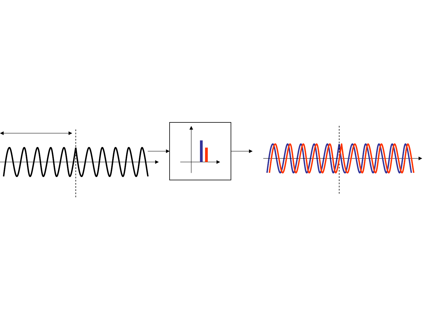
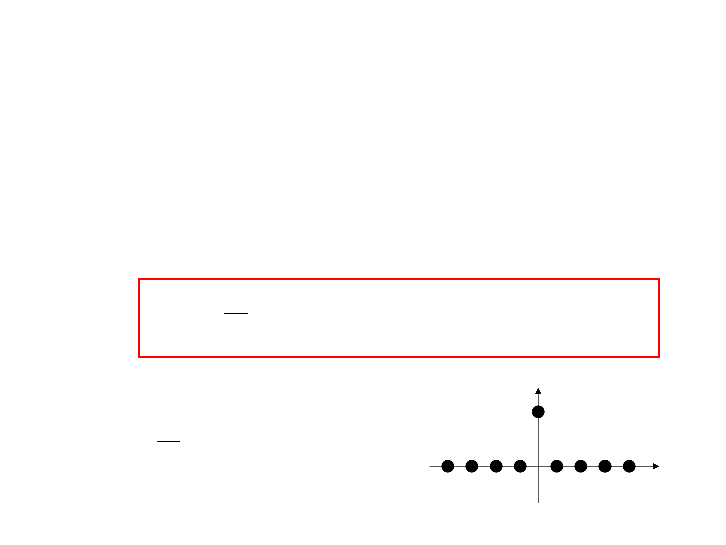
2. Single Carrier Modulation in Flat Fading Channels:
•if symbol duration >> time spread then there is almost no Inter Symbol
Interference (ISI).
10
time
channel
10
phase still recognizable
S
T
Problem with this: Low Data Rate!!!

• this corresponds to Flat Fading
Frequency
Frequency
channel
S
T/1
Flat Freq. Response
Frequency

3. Single Carrier Modulation in Frequency Selective Channels:
•if symbol duration ~ time spread then there is considerable Inter
Symbol Interference (ISI).
10
time
channel
??
phase not recognizable

One Solution: we need equalization
10
time
channel equalizer
10
time
Channel and
Equalizer
Problems with equalization:
• it might require training data (thus loss of bandwidth)
• if blind, it can be expensive in terms computational effort
• always a problem when the channel is time varying
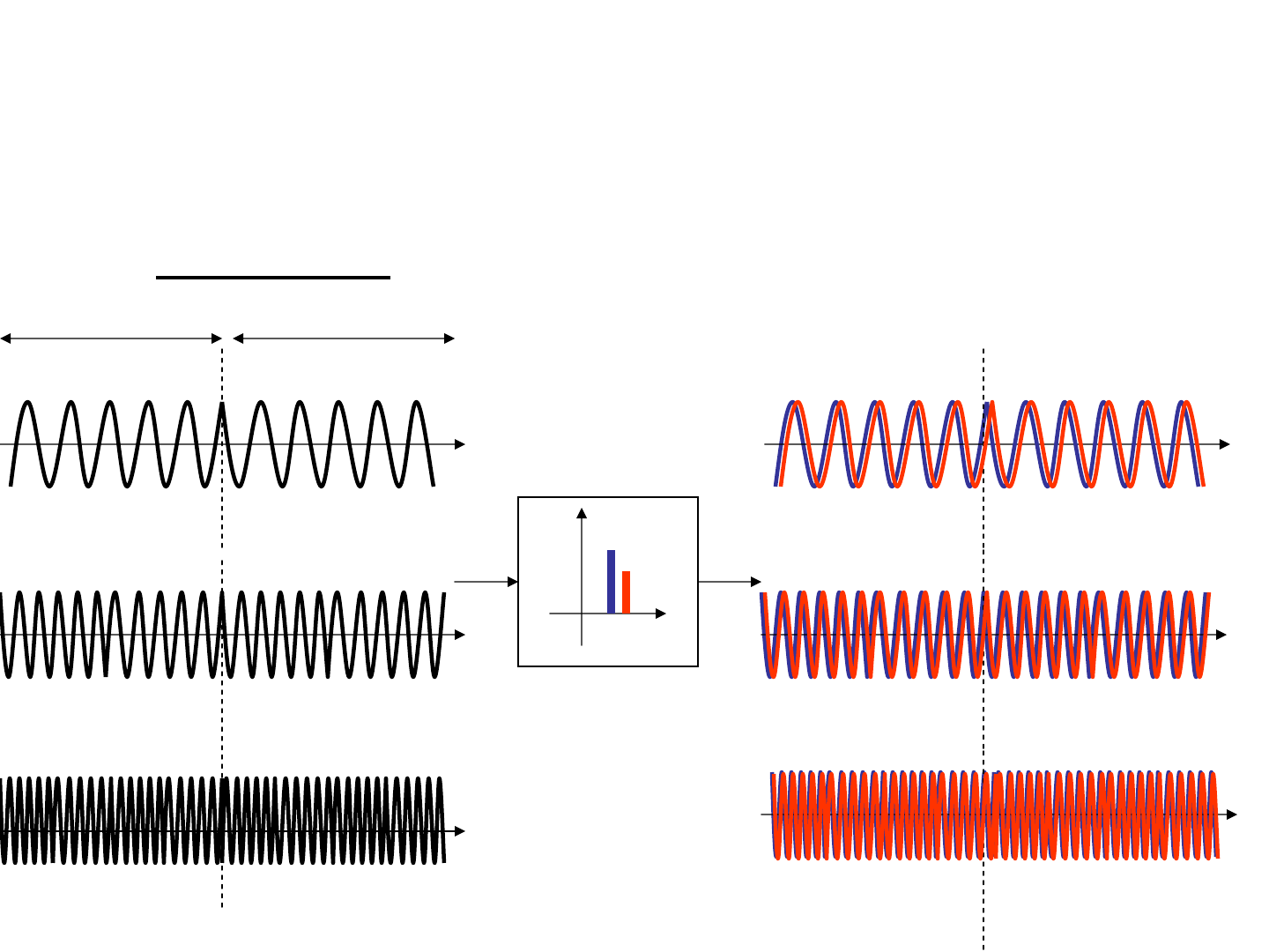
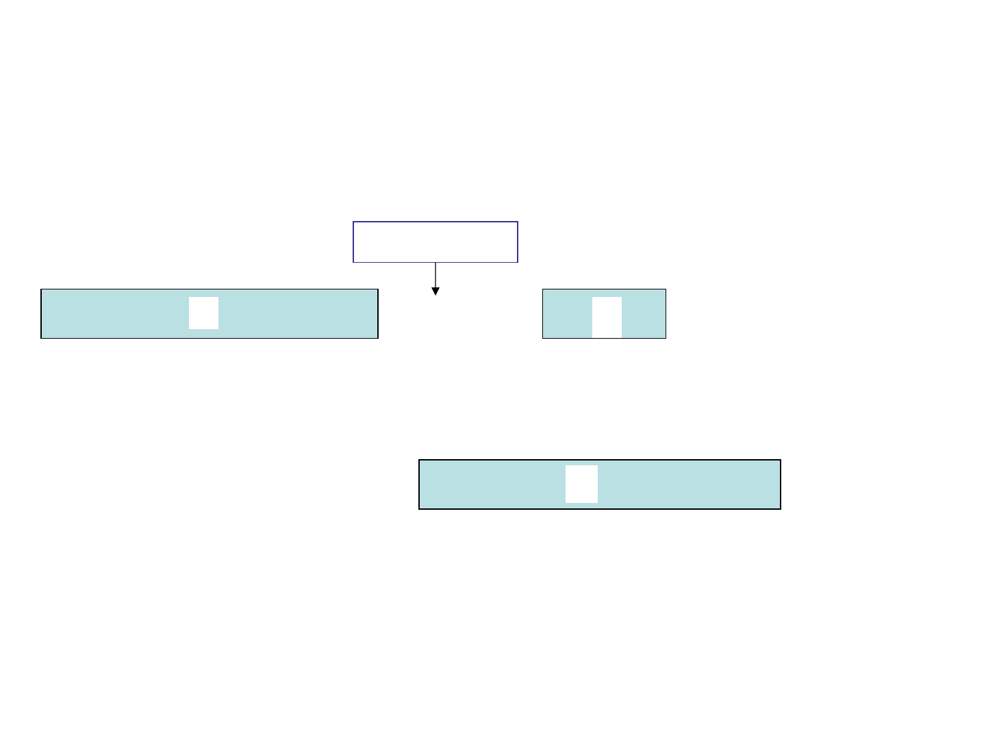
4. The Multi Carrier Approach:
•let symbol duration >> time spread so there is almost no Inter Symbol
Interference (ISI);
• send a
block of data using a number of carriers (Multi Carrier)
1
0
time
channel
time
time
0
0
1
1
“symbol” “symbol”

Compare Single Carrier and Multi Carrier Modulation
Frequency
Frequency
channel
0 1 0 1 1 1
Block of
symbols
subcarriers
Each subcarrier sees
a Flat Fading
Channel: Easy
Demod
MC
Frequency
1
One symbol
Frequency
Flat Fading Channel:
Easy Demod
SC
101 1
LL
0 1 0 1 1 1
LL

Orthogonal Frequency Division Multiplexing (OFDM)
1. Basic Structure of Multi Carrier Modulation
2. “Orthogonal” Subcarriers and OFDM
3. Generating the OFDM Symbol using the IFFT

In MC modulation each “MC symbol” is defined on a time interval and it contains a
block of data
g
T
b
T
Symbol
T
data interval
t
guard interval
()
⎪
⎭
⎪
⎬
⎫
⎪
⎩
⎪
⎨
⎧
=
⎪
⎭
⎪
⎬
⎫
⎪
⎩
⎪
⎨
⎧
=
∑∑
−=
Δ
−=
Δ+
2
2
2
2
2
2
2
ReRe)(
F
F
C
F
F
C
N
N
k
Ftkj
k
tFj
N
N
k
tFkFj
k
ecAeecAts
π
ππ
Symbol
Tt
≤
≤
0
LL
time
OFDM Symbol
data datadatadata
data
data

•Each data point is modulated by a subcarrier
c
F
c
F−
2
BW
c
F −
2
BW
c
F
+
2
BW
c
F
+
−
2
BW
c
F −−
carrier
F
|)(| FS
FkFF
Ck
Δ
+
=
FNBW
F
Δ
×
=
k
c
0,
2
,...,
2
, ≠−=Δ+= k
NN
kFkFF
FF
Ck
•Subcarrier is not used since its magnitude and phase would be influenced
by the carrier
0=k
C
F

LL
L
L
}
the “guard time” is long
enough, so the multipath in
one block does not affect the
next block
TX
RX
NO Inter Symbol Interference!
Data Block
Data Block
TX RX
We leave a “guard time”
between blocks to allow
multipath
g
T
Guard Time
b
T
Symbol
T
data+guard

∑
=
≠
−=
−Δ
=
2
2
0
)(2
)(
F
N
F
N
g
k
k
k
TtFkj
k
ecAtx
π
Modulated Signal:
frequencycarrier
=
C
F
data
=
k
c
offsetfrequency subcarrier
=
Δ
Fk
Symbol
Tt
≤
≤
0
{
}
)(Re)(
2
txets
tFj
c
π
=
Baseband Complex Signal:
just a gain
C
F
C
F−
F
FT
F
FT

Limitations of OFDM
b
T
Symbol
T
t
data
guard
T
bguard
TT
<
<
Overhead
(no data)
•To minimize overhead
ie the longer the data frame the better!
•The Guard Time (or Cyclic Prefix) does not carry data and
therefore it represents a loss of power
symbol
b
guard
symbol
guardb
b
data
P
T
T
P
TT
T
P
⎟
⎟
⎠
⎞
⎜
⎜
⎝
⎛
+
=
+
=
1
1

However, as expected, the channel (not the sky!) is the limit.
Time Spread
Frequency Spread
),( FtS
F
t
sec
μ
≈
MAX
t
kHzF
MAX
<
OFDM Symbol Duration:
MAXb
tT >>
OFDM Freq. Spacing:
MAX
S
F
N
F
F >>=Δ
Are these two compatible?
to minimize CP overhead
to ensure orthogonality
Since we have:
bS
S
TNTN
F
11
==
MAXbMAX
FTt /1
<
<
<
<
sec10
6−
sec10
3−
roughly!!!

2. “Orthogonal” Subcarriers and OFDM
g
T
b
T
data interval
t
guard interval
F
C
F
F
Δ
b
T
F
1
=Δ
FkFF
Ck
Δ
+
=
⎩
⎨
⎧
≠
=
==
∫∫
+
Δ−
+
−
l
l
l
l
k
k
dte
T
dtee
T
bb
k
Tt
t
Ftkj
b
Tt
t
tFjtFj
b
if 0
if 1
11
0
0
0
0
)(2
22
π
ππ
Choose:
Orthogonality:

)(th
t
0
tFj
k
k
eFH
π
2
)(
0
transient
response
bg
TT
+
bgg
TTtT
+
≤
≤
still orthogonal at the receiver!!!
Since the channel is Linear and Time Invariant (at least for the duration
of the frame), the exponentials are still orthogonal at the
receiver in steady state
, ie after the transient has died.
tFj
k
e
π
2
tFj
k
e
π
2
g
T
steady state
response
bg
TT +
Transmitted
subcarrier
channel
Received
subcarrier

Each OFDM symbol is generated in discrete time.
Let
• be the sampling frequency;
• be the number of data samples in each symbol;
• the subcarriers spacing
• A=1/N
Then:
S
F
()
NFTNF
SS
//1 ==Δ
∑∑
−=
−
−=
−
==
Δ
2
2
)(
2
2
)(2
2
11
)(
F
F
N
F
F
s
F
F
N
N
k
Lnjk
k
N
N
k
Lnkj
kS
ec
N
ec
N
nTx
π
π
1,..,0
−
+
=
NLn
F
NN >
With the guard time.
Sg
TLT ×=

SS
FT /1
=
t
0
g
T
L
b
T
F
NN >
Sampling Interval
guard data
OFDM Symbol: discrete time
TIME:
NFF
S
/=
Δ
F
N
F
N
S
F
2
−
Freq spacing
FREQUENCY:
2/
S
F
2/
S
F
−
N
F
N
S
F
2
0
4. Generating the OFDM symbol using the IFFT
# samples
# subcarriers
Sampling Frequency
BandwidthF
S
>

This can be written as
{}
][][
1
11
1
][
1
0
1
2
)(
2
1
2
2
2
22
2
kXIFFTekX
N
ec
N
ec
N
ec
N
Lnx
N
k
njk
N
k
nkNj
k
N
k
njk
k
N
N
k
njk
k
N
F
N
F
N
F
F
N
∑
∑∑
∑
−
=
−
−=
+
=
−=
==
+=
=+
π
ππ
π
otherwise ,0][
2/,...,1 ,][
2/,...,1 ,][
=
−−==+
=
=
kX
NkckNX
NkckX
Fk
Fk
Where:
positive subcarriers
negative subcarriers

][][ nNxnx
+
=
{
}
1,...,0],[]1[],...,[
−
=
=
−
+
NkkXIFFTNLxLx
N
0
L
1
−
+
NL
43421
43421
CP from the periodicity:
]1[]1[
...
]1[]1[
][]0[
−+=−
+=
=
NLxLx
Nxx
Nxx
⇒
Guard Time with Cyclic Prefix (CP)
IFFT{ X }CP

M
IFF
T
k
n
0 0
1−N
0
0
0
1
c
1
(
)
2/
F
N
M
2/
F
N
c
1
−
N
(
)
2/
F
NN
−
M
1−
c
2/
F
N
c
−
data
1
−
N
M
][Lx
]1[
−
+
NLx
M
OFDM Symbol
]1[]1[
−
+
=
−
LNxLx
][]0[ Nxx
=
M
Cyclic
Prefix

Summary of OFDM
… and relevant parameters
Channel (given parameters):
1. Max Time Spread
t_MAX in sec
2. Doppler Spread
F_D in Hz
3. Bandwidth
BW in Hz
OFDM (design parameters):
1. Sampling Frequency Fs>BW in Hz
2. Cyclic Prefix
L > t_MAX * Fs, integer
3. FFT size (power of 2) 4*L<
N<<Fs/F_D, integer
4. Number of Carriers
NF=[N*BW/Fs], integer

Test in Simulation:
][nh
][nw
OFDM
TX
OFDM
RX
]0[
m
X
][kX
m
]1[ −NX
m
]0[
m
Y
][kY
m
]1[
−
NY
m
M
M
M
M
m-th data
block
(data, pilots
and nulls)
⎪
⎪
⎩
⎪
⎪
⎨
⎧
Recall that for every transmitted block of data we receive
][][][][ kWkXkHkY
mmmm
+
=
With the frequency response of the channel within the time block
][kH
m
In order to estimate we need to know the channel.
][kX
m

A way to avoid it is to use differential encoding:
][kd
m
Data:
][][][
1
kXkdkX
mmm −
=
Delay
one
frame
][
1
kX
m−
With QPSK it is equivalent to accumulating the phase
][][][
1
kdkXkX
mmm
∠
+
∠
=
∠
−

][
][][][
][][][
][
][
][
ˆ
1111
kd
kWkXkH
kWkXkH
kY
kY
kd
m
mmm
mmm
m
m
m
≅
+
+
==
−−−−
Provided:
a. The channel changes slowly
b. High SNR
0][][
1
≠
≅
−
kHkH
mm
At the receiver
][kd
m
Delay
one
frame
][
1
kY
m−
][kY
m
div

Lab 4: Single Carrier vs. OFDM Modulation
Goal: In this Lab we want to compare Single Carrier (SC) modulation
with Orthogonal Frequency Division Multiplexing (OFDM), with
Differential Modulation .
1. Using the Simulink model test_SC.mdl see the received signal for
various values of the symbol rate
kHzF
S
0.2000,0.200,0.20,0.2
=
As the symbol rate increases, notice the effect of Inter Symbol
Interference in the scattering plot.
2. Repeat the same with the Simulink model test_OFDM.mdl and see
the received signal for the same values of the symbol rate. Notice how
you can increase the data rate and still be able to demodulate the
received signal.

Example: IEEE 802.11a (WiFi)
1. Parameters
2. Simulink Example
3. “Frame based” and “Sample based”
signals

Parameters of IEEE802.11a:
Channel (given parameters):
1. Max Time Spread
t_MAX=0.5 microsec
2. Doppler Spread F_D=50Hz
3. Bandwidth BW=16MHz
OFDM (design parameters):
1. Sampling Frequency Fs=20MHz
2. Cyclic Prefix L=16 > 0.5*20=10
3. FFT size (power of 2)
N=64<<20e06/50
4. Number of Carriers
NF=52=[64*16/20]

Sub-carriers: (48 data + 4 pilots) + (12 nulls) = 64
0
1
26
38
63
M
M
M
NULL
NULL
0
63
M
M
M
M
Frequency Time
1
c
26
c
26−
c
1−
c
0
x
63
x
IFFT
Pilots at: -21, -7, 7, 21
52=
F
N
64
=
N

k
26
38
(
)
64 26−
20 /64 312.5FMHz kHz
Δ
==
()
F
MHz
L
L
8.1258.125
−
CARRIER
F
)(MHzF
MHz25.16
DATA
Frequencies:
s
TMHz /120
=
1
63
Subcarriers index
10−
CARRIER
F
10
+
CARRIER
F

Time Block:
sec2.3
μ
=
FFT
T
sec105064/
9−
×==
FFTs
TT
sec8.0
μ
=
G
T
sec0.4
μ
=
FRAME
T
time

Overall Implementation (IEEE 802.11a with 16QAM).
1. Map encoded data into blocks of
192 bits and 48 symbols:
data
Encode
Interleave
…010011010101…
Buffer
(192 bits)
1110
0111
1000
…
1101
4x48=192 bits
Map to
16QAM
…
48
4
+1+j3
-1+j
+3-j3
…
+1-j
a
l
48

Overall Implementation (IEEE 802.11a with 16QAM).
2. Map each block of
48 symbols into 64 samples
[]
m
X
k
+1+j3
…
-3-j
+3-j3
…
+1-j
M
0
1
26
27
6427
+
−
M
M
6426
+
−
M
[0]
m
x
IFFT
0
1
2
63
62
time domain
frequency domain
null
null
⎩
⎨
⎧
⎩
⎨
⎧
⎩
⎨
⎧
24 data
2 pilots
24 data
2 pilots
⎭
⎬
⎫
⎭
⎬
⎫
M
LL
k
1
26
26−
641
+
−
1−
[]
m
a l []
m
x
n
1:48=l 0:63k
=
0:63n
=
[1]
m
x
[62]
m
x
[63]
m
x

Simulink Example
To make it simpler:
1. let the number of carrier be the same as the FFT length, ie
N=NF;
2. Use Differential QPSK Encoding and Decoding, so that we do
not need to estimate the channel’s frequency response.

Initial Callback function:
% OFDM parameters (IEEE802.11a)
Fs=20e6; % symbol data rate (uncoded) in Hz
N=64; % FFT sample size
L=16; % Cyclic Prefix sample length
% Channel Parameters
% 1. Doppler Spread
FC=5.0; % carrier freq. in GHz
v=50; % speed in km/h
FD=v*FC; % doppler freq in Hz
%2. Time Spread
tau=[0, 0.1, 0.4]*1e-6; % time delays in seconds
P=[0, -2, -4]; % attenuations in dB
% Additive Noise
SNRdB=20; % dB

Simulink Implementation of OFDM IEEE802.11a
Recall how we compute the IFFT at the Modulator
0
1
26
38
63
M
M
M
NULL
NULL
0
63
M
M
M
M
1
d
26
d
27
d
52
d
)1(x
)64(x
IFFT
Block of 52 data
points (data + pilots)
CP
)49(x
)64(x
)1(x
)64(x
Block of 80 samples
IN:
OUT:
M
M
M
Recall: vectors in
Matlab begin at n=1

Vector operations.
OFDM Modulator
:
52 data points
(include the pilots)
26
26
1
110
0
IFFT
64
ADD CP
80
Split
Data
26
26
52
Transmitted FrameConcatenate
in a vector

OFDM Modulator:
Simulink > Commonly
Used Blocks > demux
Simulink > Math Operations > Matrix
Concatenate
Simulink > Signal Routing > Selector
repeat last 16 entries
[49:64, 1:64]

OFDM Demodulator:
80
Remove
CP
26
26
1
11
FFT
64
Concatenate
in a vector
26
26
52
Received Frame
Received Data

Simulink > Signal Routing > Selector
Signal Processing >
Signal Management >
Signal Attributes
demux
Simulink > Math Operations > Matrix
Concatenate
Simulink > Commonly Used
Blocks > Terminator

Put Everything Together:
Differential enc/dec
M=4 (QPSK)
f_D=doppler freq.

3. “Frame based” and “Sample based”
In Simulink a signal can be
• Frame based
• Sample based
This is particularly important when the signals are vectors.
• Some blocks want the input to be Frame based, others want it Sample
based, others don’t care
• When you have to process a large number of data, it is more efficient to
process blocks of samples, using Frames, rather than one sample at a
time.

Frame Based [Nx1]
N
“Frame based”
Each vector is part (a “frame”) of the same signal

Sample Based [Nx1]
N
“Sample based”
There are N different signals. Each element of the vector
belongs to a different signal.

Typical Example: the FFT block
FFT
To
Frame
[Nx1]
[Nx1]
[Nx1]
frame sample
frame

IEEE 802.16 Standard
IEEE 802.16 2004:
Part 16: Air Interface for Fixed Broadband Wireless Access
Systems
From the Abstract:
• It specifies air interface for fixed Broadband Wireless Access (BWA) systems
supporting multimedia services;
• MAC supports point to multipoint with optional mesh topology;
• multiple physical layer (PHY) each suited to a particular operational environment:

IEEE 802.16-2004 Standard
• WirelessMAN-SC, Single Carrier (SC), Line of Sight (LOS), 10-66GHz, TDD/FDD
• WirelessMAN-SCa, SC, 2-11GHz licensed bands,TDD/FDD
• WirelessMAN OFDM, 2-11GHZ licensed bands,TDD/FDD
• WirelessMAN-OFDMA, 2-11GHz licensed bands,TDD/FDD
• WirelessHUMAN 2-11GHz, unlicensed,TDD
MAN: Metropolitan Area Network
HUMAN: High Speed Unlicensed MAN
Table 1 (Section 1.3.4) Air Interface Nomenclature:

IEEE 802.16e 2005:
Part 16: Air Interface for Fixed and Mobile Broadband
Wireless Access Systems
Amendment 2: Physical and Medium Access Control Layers
for Combined Fixed and Mobile Operation in Licensed
Bands
and
Corrigendum 1
Scope (Section 1.1):
• it enhances IEEE 802.16-2004 to support mobility at vehicular speed, for combined
fixed and mobile Broadband Wireless Access;
• higher level handover between base stations;
• licensed bands below 6GHz.

IEEE 802.16-2004: Reference Model (Section 1.4), Figure 1
By Layers:
Service Specific Convergence
Sublayer (CS)
CS-SAP
SAP=Service Access Point
MAC Common Part Convergence
Sublayer (CS)
MAC-SAP
Security Sublayer
Physical Layer
PHY-SAP
MAC
PHY
Section 5
Section 6
Section 7
Section 8
External Data

Parameters for IEEE 802.16 (OFDM only)
(1,2,4,8)x1.75MHz
(1,4,8,12)x1.25MHz
8.75MHz
(1,2,4,8)x1.75MHz
(1,4,8,12)x1.25MHz
8.75MHz
Channel Bandwidth
TDD or FDDTDD or FDDDuplexing
1Mbps-75Mbps1Mbps-75MbpsTransmission Rate
QPSK, 16QAM, 64QAMQPSK, 16QAM, 64QAMModulation
OFDM: 256
OFDMA: 128, 256, 512,1024,
2048
OFDM: 256
OFDMA: 2048
OFDM carriers
2GHz-11GHz fixed
2GHz-6GHz mobile
2GHz-11GHzFrequency Band
802.16e-2005802.16-2004

randomization
data
Error
Correction
Coding
TX
IEEE802.16 Structure
M-QAM
mod
OFDM
mod
De-rand.
data
Error
Correction
Decoding
RX
M-QAM
dem
OFDM
dem
3/4
5/6
2/3
1/2
Coding rates
16
64
4
2
M-QAM
1024
2048
512
256
OFDM
carriers
Choices:
10 MHz
…
5 MHz
1.25 MHz
Channel
B/width

OFDM and OFDMA (Orthogonal Frequency Division Multiple Access)
• Mobile WiMax is based on OFDMA;
• OFDMA allows for subchannellization of data in both uplink and downlink;
• Subchannels are just subsets of the OFDM carriers: they can use contiguous or
randomly allocated frequencies;
• FUSC: Full Use of Subcarriers. Each subchannel has up to 48 subcarriers evenly
distributed through the entire band;
• PUSC: Partial Use of Subcarriers. Each subchannel has subcarriers randomly
allocated within clusters (14 subcarriers per cluster) .

Section 8.3.2: OFDM Symbol Parameters and Transmitted Signal
OFDM Symbol
g
T
b
T
s
T
dataguard
(CP)
Cyclic Prefix has a variable length. It represents a loss of
(
)
)/(log10
gbbCP
TTTL +
=
11 1 1
,, ,
481632
g
b
T
T
=

An OFDM Symbol is made of
• Data Carriers: data
• Pilot Carriers: synchronization and estimation
• Null Carriers: guard frequency bands and DC (at the modulating carrier)
channel
frequency
pilots
data
Guard
band
Guard
band
to provide frequency guards between channels
1 (DC subcarrier is always zero)
pilots for channel tracking and synchronization
data subcarriers
guards
nulls guards
pilots
data
used pilots dat
N
NN
N
N
NN N
=
=+
=
=
=+
a

Recall the OFDM symbol is of the form
⎪
⎭
⎪
⎬
⎫
⎪
⎩
⎪
⎨
⎧
=
∑
=
≠
−=
−Δ
2
2
0
)(2
2
Re)(
used
N
used
N
g
c
k
k
k
Ttfkj
k
tfj
ecets
π
π
c
f
c
f−
2
BW
c
f −
2
BW
c
f
+
2
BW
c
f
+
−
2
BW
c
f −−
carrier
f
|)(| fS

153676838496192N_data
1668242128N_pilots
346174862056N_nulls
1702850426108200N_used
20481024512128256FFT size
OFDM Subcarrier Parameters:
Fixed
WiMax
444444344444421
Fixed and
Mobile
WiMax

In 802.16 2004 we have
200
256
=
=
used
FFT
N
N
fNF
FFTs
Δ
=
2
s
F
2
s
F
−
2
BW
2
BW
−
s
FFT
used
used
F
N
N
fNBW
=Δ=
Sampling frequency
Bandwidth
Since we want the sampling rate to be integer multiple of a fixed rate (say
8kHz), the formula for the sampling rate is
(
)
000,8000,8/
×
×
= BWnfloorF
s
With n a factor (Table 213) of the order
200
256
,
50
57
,
275
316
,
125
144
,
75
86
,
7
8
≈=n
Frequency Spacing
b
Tf /1l_lengthdata_symbo/1 =
=
Δ

IEEE 802.16, with N=256
0
100
155
255
M
M
M
13
38
88
63
168
218
193
243
101
M
][ Lnx
+
][kX
0
255
IFFT
data
pilots
nulls
12
24
24
24
12
12
12
24
24
24
↓
k
↓
n
156

Implementation of WiMax 2004 in Simulink
NFFT=256
NCP=64
Data in 192x1

5. Error Correcting Coding
1. Channel Capacity and Error Correction Coding
2. Block Coding
3. Code Shortening and Puncturing
4. Simulink Implementation of Block Codes
5. Convolutional Codes
6. Simulink Implementation of Convolutional Codes
7. Concatenated Codes in IEEE802.16

1. Channel Capacity and Error Correction Coding
1.1 Channel Capacity
1.2 Error Correction Coding
1.3 Minimum SNR Requirement
and Shannon Limit

1. Channel Capacity
Problem: given a AWGN Channel, defined in terms of
•
Signal to Noise Ratio (SNR)
• Bandwidth B
and a desired Bit Error Rate (BER),
what is the
maximum data rate we can transmit?
channel
..01010110…
Errors!
..01010010…
MOD DEM
noise
Transmitted Received

(
)
SNRBC
+
=
1log
2
bits/sec
Significance: if the transmitted data rate R<C then we can always
find a coding scheme to make the bit error rate arbitrarily small.
Define the
Channel Capacity:
Example:
SNRdB=20dB
B=10MHz
⇒
(
)
sec/5.66101log10
10/20
2
7
MbitsC =+=
Problem: How do we encode the data to obtain an acceptable error rate?
Use Error Correction Coding!

2. Error Correction Coding
Purpose: detect and Correct Errors by adding redundant information.
How to Define an Encoder:
• code rate
u
R
ue
RR >
encoder
data rate
1<=
e
u
c
R
R
r
c
r
• number of errors corrected
Encoded data
rate
bits of # total
errorin bits #
=BER

Relation to Channel Capacity
C
CR
u
<
encoder
c
r
channel
SNR
C
decoder
c
r
u
R
B
ER
Given
• a data rate
•a desired Bit Error Rate (BER) arbitrarily small
you can always find a code
with coding rate
1<≤
C
R
r
u
c
CR
u
<
with desired BER.

Clearly the Complexity goes up with the coding rate.
c
r
16/15
Code
Complexity
$$$
code rate
Example
: see two situations with the same and
5
10
−
=BER
A. Convolutional Encoder with rate
B.
Block Code (65520, 61425) low density parity check, with coding
rate
2/1
=
c
r
dBNE
b
4/
0
≈
16
15
65520
61425
==
c
r
2/1

For a given Coding Rate, what is the minimum we can have?
0
/ NE
b
dB
N
E
b
6.1
0
−>
3. Minimum SNR Requirements
-2 -1 0 1 2 3 4 5 6 7 8
0
0.1
0.2
0.3
0.4
0.5
0.6
0.7
0.8
0.9
1
Shannon Limit
EbN0 dB
coding rate
dB6.1−
Notice: always!!!

2. Block Coding
2.1 Parameters of Block Codes
2.2 Probability of Error
2.3 Reed Solomon Codes (non binary data)
2.3 Simulink Implementation

1. Parameters of Block Codes
encoder
raw data
encoded data
k symbols
n> k symbols
Code Rate
n
k
r
c
=
),,( tkn
It encodes k blocks of data symbols into n blocks of encoded symbols:
Parameters
:
),,( tkn
Max. number of errors corrected
⎟
⎠
⎞
⎜
⎝
⎛
−
≤
2
1
min
d
floort
1
min
+
−
≤
knd
where
Minimum distance between codewords

codewords
non -codewords
L
L
min
d
t
A
B
C
D
A
transmit
receive
decode
channel decoder
C
A
D B
Error !!!
where
tADd
tACd
>
≤
),(
),(

If the code corrects up to t errors, the probability that the wrong
codeword is decoded is given by
()
2/
1
min
)1(4)12()1(
d
k
n
tj
jnj
e
pppp
j
n
P −−≤−
⎟
⎟
⎠
⎞
⎜
⎜
⎝
⎛
≤
∑
+=
−
“j” bits wrong
“n-j” bits right
with p the probability of error for one bit.
(
)
0
/2 NEQp
c
=
For BPSK, QPSK:
bc
E
n
k
E Bit Coded ofEnergy ==
2. Probability of Error
k
P
pp
j
n
jP
e
n
tj
jnj
b
≈−
⎟
⎟
⎠
⎞
⎜
⎜
⎝
⎛
≈
∑
+=
−
1
)1(
Bit Error Probability for HDD
codeword error
bits per codeword

4 5 6 7 8 9 10 11
-7
-6.5
-6
-5.5
-5
-4.5
-4
-3.5
-3
-2.5
-2
Eb/N0 dB
log10(Prob of error)
Probability of Error: BPSK coded and uncoded
Some Probabilities of Error for BPSK:
Uncoded
Golay (24,12,3)
BCH (127,64,10)

⎟
⎟
⎠
⎞
⎜
⎜
⎝
⎛
−
=
2
2 k
floort
m
Good for Burst Error Correction at relatively high SNR
3. Reed Solomon Codes (non Binary Data)
Example: (255,239,8)
239 symbols
255 symbols
RS
(
)
tkn ,,
12 −=
m
n
coded symbols
k<n uncoded
symbols
errors corrected
1 symbol = m bits
239 symbols
=
16
data
parity

Based on polynomials:
RS
uncoded block
coded block
]1[],...,0[ −kuu ]1[],...,0[
−
ncc
1
]1[...]1[]0[)(
−
−+++=
k
XkuXuuXu
1
]1[...]1[]0[)(
−
−+++=
n
XncXccXc
)()()( XuXgXc
=
)(Xu
)(Xg
encoder
)(Xe
errors
)()()(
)()()(
XeXuXg
XeXcXy
+=
+
=
)(
)(
Xg
Xy
)(Xu
)(Xe
quotient
remainder

3. Code Shortening and Puncturing
3.1 Code Shortening
3.2 Code Puncturing
3.3 RS Coding in IEEE802.16

1. Code Shortening
Start with a block code, say RS (n=255, k=239, t=8).
We can generate a different code by
Shortening:
1. Shortened to k’ data bytes by adding 239-k’ null symbols
2. At the output eliminate the corresponding 239-k’ terms
k’
(255, 239,8)
16 00000
239 symbols
k’ 00000
255 symbols
(k’+16,k’,8)
k’ k’ 16

By shortening Reed Solomon (255,239,8) we obtain codes
()
,8,',16' kk
+
All these codes correct up to 8 errors (bytes).
239'0
≤
<
k
(k’+16,k’,8)
k’ k’ 16

By puncturing we eliminate L parity bytes to obtain a code correcting
8-T errors. Therefore we determine L from
()
TLT
L
T
kN
28
2
16
8
2
=⇒−=
−
⇒−=
−
}
bytesparity
2. Code Puncturing

Puncturing Reed Solomon Codes
1. The last 16 bytes are parity bytes
2. For a code, correcting 8-T errors, just eliminate
the first 2T bytes of the parity check.
()
TkTk
−
−+ 8,',216'
()
8,',16' kk +
Code:
(
)
,8,',16' kk
+
239'0
≤
<
k
(k’+16,k’,8)
k’ k’ 16
(k’+16,k’,8-T)
k’ k’
()
TkTk −−+ 8,',216'
16-2T parity

RS codes used in IEEE802.16:
(32,24,4)
(40,36,2)
(64,48,8)
(80,72,4)
(108,96,6)
(120,108,6)
k’=24, T=4
k’=36, T=6
k’=48, T=0
k’=72, T=4
k’=96, T=2
k’=108, T=2
(
)
TkTk
−
−
+
8,',216'

4. Simulink Implementation of Block Codes
4.1 Shortened Codes
4.2 Punctured Codes

Simulink Implementation of Shortened RS Codes
Let’s implement the code (52,36,8) by shortening
1. Shortened to k’=36 data bytes (=36x8=288 bits) by adding 239-k’
null symbols at the beginning of the block
2. At the output eliminate the first 239-k’ terms
36
20336239
=
−
52
203
255239
RS
bits to
symbols
symbols
to bits
8 bits/symbol
8 bits/symbol
288 bits
416 bits

RS Encoder
Raw data
288 bits
Encoded data
416 bits

RS Decoder
Raw data
288 bits
Received data
416 bits
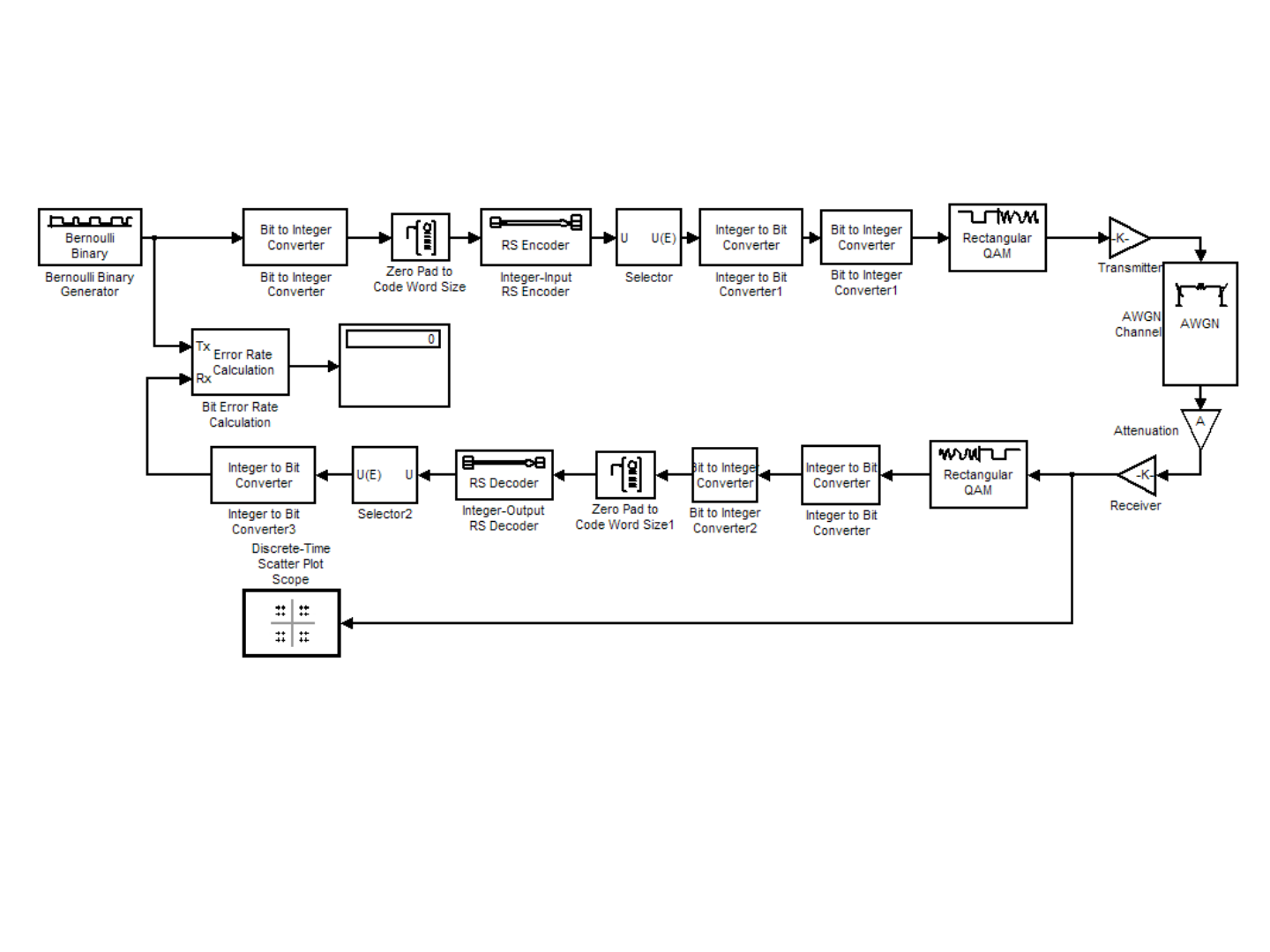
Put Everything together:

It is easier to create subsystems:
RS encoder
RS decoder
MQAM Mod
MQAM Demod
Channel
Select each group of blocks and use
Edit > Create Subsystem
It cannot be undone!


Masked Subsystems
In Simulink we can create customized blocks, where we can enter
parameters values.
Example: Reed Solomon Encoder and Decoder
data
'n
encoded
data
RS
Encoder
RS
Decoder
datablock

[239-k+1:255]
RS Encoder:
1. edit
2. right click on subsystem and select Mask Subsystem
3. Edit Mask:
add parameters

You can customize the icon
When you “click” on the icon, you get the following:
the two
parameters from
previous slide
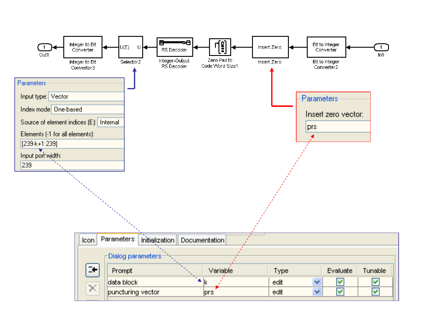
RS Decoder:
2. right click on subsystem and select Mask Subsystem
3. Edit Mask:

Simulink Implementation of (40,36,2).
1. Start with the previous code (52,36,8);
2. Puncture
it by eliminating 2T=12 (ie T=6) bytes in the parity

RS (40,36,2) encoder
RS (40,36,2) decoder
Sequence Operations>Puncture
same vector
Sequence Operations>Insert Zero
Eliminate last 12 bytes
Insert 12 zeros
Convolutional Encoders
1. Definition of Convolutional Encoders
2. Puncturing
3. Simulink Implementation

Convolutional Encoders
M
M
k
n
CC
L
L
LL
n
k
Rate
raw data
Coded data
It continuously updates k data symbols into n>k coded symbols.

Example: a 2/3 encoder
1−
z
1−
z
1−
z
1−
z
1−
z
1−
z
1−
z
1
x
2
x
1
y
2
y
3
y

Polynomial description:
1−
z
1−
z
1−
z
1−
z
1−
z
1−
z
1−
z
1
x
2
x
1
y
2
y
3
y
[][]
⎥
⎦
⎤
⎢
⎣
⎡
=
232221
131211
21321
aaa
aaa
xxyyy
111
1
1
1
1
11
1
11
00
00
0
0
23)011()10(
8811
=
=
→ a
35)101()11(
8812
=
=
→ a
5)101()0(
8822
=
=
→ a
13)011()1(
8823
=
=
→ a

[][]
⎥
⎦
⎤
⎢
⎣
⎡
=
1350
03523
21321
xxyyy
Therefore the code is described by the matrix (all entries are octal)
no connection
31
yx →
no connection
12
yx →
The parameters are then:
CONSTRAINED_LENGTH = [4,3]
CODEGENERATOR=[23,35,0; 0,5,13]
which call the function “poly2trellis”

In IEEE802.16e the Convolutinal Code has rate ½ and constrained
length 7:
1−
z
1−
z
1−
z
1−
z
x
1
y
2
y
1−
z
1−
z
],[],[
2121
aaxyy =
7length dconstraine
133)011()011()1(
171)001()111()1(
8882
8881
=
==
=
=
a
a

Note: in some books (as in [Costello]) the binary coefficients are
determined in reverse order.
Example: the code in the previous page is defined by he polynomials
(begin counting from the right
) as
(
)
(
)
(
)
()()()
1550110111
1171110011
888
2
888
1
==
=
=
g
g

Punctured Codes
From an (k,n) convolutional code make a code with higher rate (less
correcting capabilities), by periodically eliminating output bits.
Example in IEEE 802.16e:
The code [171,133] seen before is a (1,2) code:
KK ],[, nx
KK ],[],[,
21
nyny
encoder

KK ],[],1[, nxnx −
KK ],[],[],1[],1[,
2121
nynynyny
−
−
encoder
Rate 2/3:
We can represent it as a matrix with 2 rows:
⎥
⎦
⎤
⎢
⎣
⎡
=
11
01
P
KK ],[],[],1[],1[,
2121
nynynyny
−
−
1
1
0
1
Since:

KK ],[],1[],2[, nxnxnx −−
KK ],[],[],1[],1[],2[],2[,
212121
nynynynynyny
−
−
−
−
encoder
Rate 3/4:
We can represent it as a matrix with 2 rows:
⎥
⎦
⎤
⎢
⎣
⎡
=
011
101
P
1
1
0
1
Since:
KK ],[],[],1[],1[],2[],2[,
212121
nynynynynyny −
−
−
−
1
0

KK ],[],1[],2[],3[],4[, nxnxnxnxnx
−
−−−
KK ],[],[],1[],1[],2[],2[],3[],3[],4[],4[,
2121212121
nynynynynynynynynyny
−
−
−
−
−
−
−−
encoder
Rate 5/6:
We can represent it as a matrix with 2 rows:
⎥
⎦
⎤
⎢
⎣
⎡
=
01011
10101
P
1
1
0
1
Since:
1
0
KK ],[],[],1[],1[],2[],2[],3[],3[],4[],4[,
2121212121
nynynynynynynynynyny
−
−
−
−
−
−
−−
0
1
0
1

Simulink Implementation
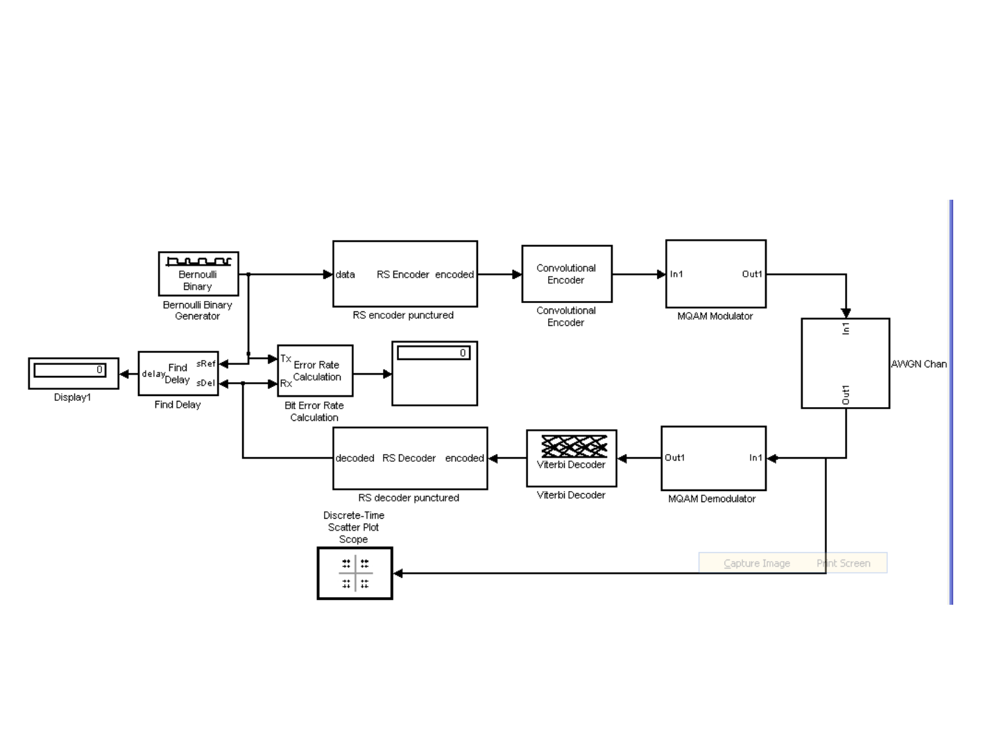
Implementation of Concatenated Codes using Simulink
AWGN_RSCC_masked.mdl

Variable DataRates with Concatenated Codes in IEEE802.16
• It is highly desirable to be able to set the system to a number of different data and
coding rates to adapt to channel conditions;
•IEEE802.16 achieves variable data rates by a combination of mechanisms:
• coding (shortening, puncturing)
• data block length (subchannelization)
• different rates have to be easily achieved by changing appropriate parameters
without major reconfigurations.
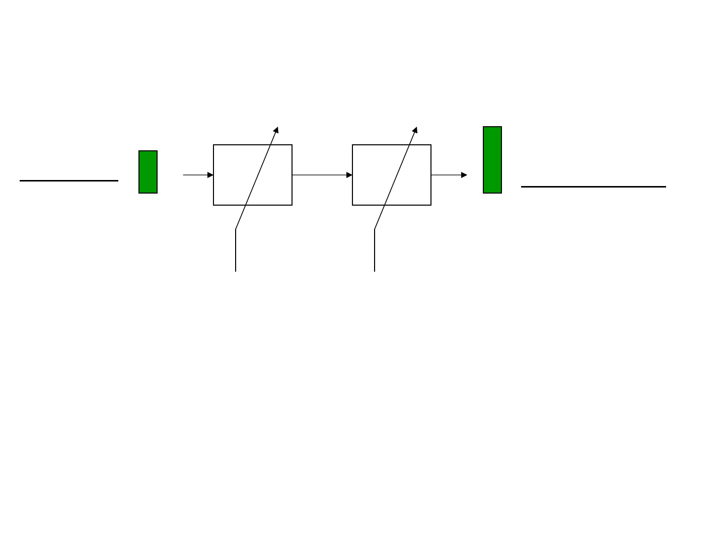
Recall from previous units:
k
RS
encoder
CC
encoder
RS
n
n
Raw Data in
Encoded Data out
RS parameters CC parameters
• encoder/decoder
• reduction
• puncturing
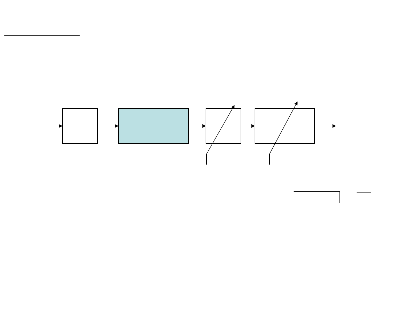
Zero
Pad
RS
(255,239,8)
select puncture
k
239 255
16
+
k
Tkn
RS
216
−
+
=
]0,...,0,1,...,1[
=
RS
p
321
321
Tk 216
−
+
T
2
RS Encoder
k
()
TkTk
−
−
+ 8,,216

Convolutional Encoder with coding rate
RS
n
CC
[171,133]
puncture
RS
n2
CC
RS
r
n
n =
CC
r
]0,1,1,0,0,1,1,0,1,1[,6/5
]0,1,1,0,1,1[,4/3
]1,0,1,1[,3/2
]1,1[,2/1
==
==
==
=
=
Pr
Pr
Pr
Pr
CC
CC
CC
CC

By combining the two codes we obtain a number of data rates (section 8.3.3.2 of the
standard):
5/6(120,108,6)3/4144108646
3/4(108,96,6)2/314496645
5/6(80,72,4)3/49672164
2/3(64,48,8)1/29648163
5/6(40,36,2)3/4483642
2/3(32,24,4)1/2482441
1/2(12,12,0)1/2241220
CC
coding
rate
RS CodeCoding
rate
k/n
Coded
block n
(bytes)
Data
block k
(bytes)
M-
QAM
Rate ID

Example:
take Rate_ID=2
36
RS
encoder
CC
encoder
40
48
6/5
40
=
Raw Data in
Encoded Data out
RS parameters CC parameters
5/6(40,36,2)3/4483642
CC coding
rate
RS CodeCoding rate
k/n
Coded
block n
(bytes)
Data block k
(bytes)
M-QAMRate ID
]0,...,0,1,...,1[=
RS
p
321
321
40621636 =×−+ 1262
=
×
36=k
]0,1,1,0,0,1,1,0,1,1[=
CC
p

This yields a table of parameters for each “Rate_ID”:
5/6144[1,1,0,1,1,0,0,1,1,0][ones(1,120),zeros(1,4)]108646
3/4144[1,1,0,1,1,0][ones(1,108),zeros(1,4)]96645
5/696[1,1,0,1,1,0,0,1,1,0][ones(1,80),zeros(1,8)]72164
2/396[1,1,0,1]148163
5/648[1,1,0,1,1,0,0,1,1,0][ones(1,40),zeros(1,12)]3642
2/348[1,1,0,1][ones(1,32),zeros(1,8)]2441
1/224[1,1]No RS1220
CC
coding
rate
Coded
block n
(bytes)
Data
block
k
(bytes)
M-
QAM
Rate
ID
RS
p
CC
p

All parameters can be
computed from the
matlab program
coding.m

The Coding Rates and the MQAM modulation parameters are designed in such a way
that, in all cases
symbols
M
n
192
)(2log
*8
=
Row Data
Block
k
RS
Coded Data
Block
nRS
MQAM
Symbol Block
From Data
Source
To IFFT
CC
Coded Data
Block
n
bytes:

In all cases of NFFT=256,512,1024,2048 the number of data symbols transmitted is a
multiple of 192.
Recall this table:
153676838496192N_data
1668242128N_pilots
346174862056N_nulls
1702850426108200N_used
20481024512128256FFT size
2x192 4x192 8x192

Put Everything together for IEEE802.16 2004 with AWGN Channel
WiMax256.mdl

IEEE802.16 Implementation
In addition to OFDM Modulator/Demodulator and Coding we need
• Time Synchronization: to detect when the packet begins
• Channel Estimation: needed in OFDM demodulator
• Channel Tracking: to track the time varying channel (for mobile only)
In addition we need
• Frequency Offset Estimation: to compensate for phase errors and noise in the
oscillators
• Offset tracking: to track synchronization errors

Basic Structure of the Receiver
WiMax Demodulator
Demodulated
Data
Received
Signal
Time Synchronization:
detect the beginning of
the packet and OFDM
symbol
Channel Estimation:
estimate the frequency
response of the channel

In IEEE802.16 (256 carriers, 64 CP) Time and Frequency Synchronization are
performed by the Preamble.
Long Preamble: composed of 2 OFDM Symbols
Short Preamble: only the Second OFDM Symbol
First OFDM Symbol Second OFDM Symbol
320 samples
320 samples
L
4 repetitions of a short
pulse+CP
64
2 repetitions of a long
pulse + CP
64
64
64 64 128 128
d
T
g
T
d
T
g
T
64
Time Synchronization

The standard specifies the Down Link preamble as QPSK for subcarriers between -100
and +100:
⎩
⎨
⎧
++−−=±±
=
otherwise ,0
100,...,1,1,...,100 ,1
][
kj
kP
ALL
Using the periodicity of the FFT:
100,...,1],[ =kkP
ALL
1
100
156
255
1,...,100],256[][
−
−
=
+
= kkPkP
ALLALL

64
64
64 64
][
4
kP
][
4
np
0 255
L
0 4
8
252 255
F
F
T
• Short Preamble, to obtain the 4 repetitions, choose only subcarriers multiple of 4:
⎩
⎨
⎧
=
=
otherwise ,0
04mod if ],[2
][
*
4
kkP
kP
ALL
Add Cyclic Prefix:
64
64
64 64
0
319
64
255
][
4
np

• Long Preamble: to obtain the 2 repetitions, choose only subcarriers multiple of 2 :
⎩
⎨
⎧
=
=
otherwise ,0
02mod if ],[2
][
2
kkP
kP
ALL
128
][
2
kP
][
2
np
0 255
L
0
4 8
252
255
F
F
T
2
254
6
128
Add Cyclic Prefix:
64
0
319
][
2
np
128 128
43421
CP

Several combinations for Up Link, Down Link and Multiple Antennas.
We can generate a number of preambles as follows:
⎩
⎨
⎧
=
=
otherwise ,0
02mod if ],[2
][
0
2
kkP
kP
ALL
⎩
⎨
⎧
=
=
otherwise ,0
12mod if ],[2
][
1
2
kkP
kP
ALL
⎩
⎨
⎧
=−+
=
otherwise ,0
4mod if ],2[
][
*
4
mkmkP
kP
ALL
m
⎩
⎨
⎧
=
=
otherwise ,0
04mod if ],[2
][
*
0
4
kkP
kP
ALL
3,2,1=m
0=m
With 2 Transmitting Antennas:
With 4 Transmitting Antennas:

Time Synchronization from Long Preamble
preamble OFDM Symbols
64 128 128
L
Received signal:
128−
z
xcorr
][ny
⎟
⎠
⎞
⎜
⎝
⎛
−−×
⎟
⎠
⎞
⎜
⎝
⎛
−
−−−
=
∑∑
∑
==
=
127
0
2
127
0
2
2
127
0
*
2
]128[][
]128[][
][
ll
l
ll
ll
nyny
nyny
nr
y
0
n
Compute Crosscorrelation Coefficient:
1. Coarse Time Synchronization using Signal Autocorrelation
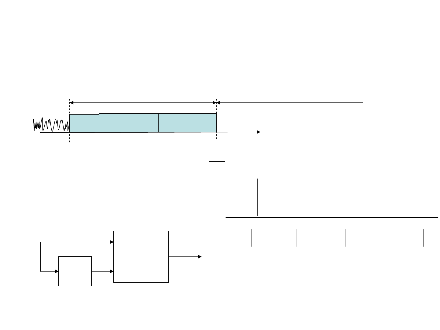
Time Synchronization from Long Preamble
preamble OFDM Symbols
64 128 128
L
Received signal:
128−
z
xcorr
][ny
⎟
⎠
⎞
⎜
⎝
⎛
−−×
⎟
⎠
⎞
⎜
⎝
⎛
−
−−−
=
∑∑
∑
==
=
127
0
2
127
0
2
2
127
0
*
2
]128[][
]128[][
][
ll
l
ll
ll
nyny
nyny
nr
y
0
n
Compute Autocorrelation :
1. Coarse Time Synchronization using Signal Autocorrelation

1
][
2
nr
y
0
n
n
MAX when
]128[][
−
=
nyny
][ny
64 128 128
L
0
n
]128[ −ny
64 128 128
L
n
n
Effect of Periodicity on Autocorrelation:
64
0
−
n

][ny
2
127
0
*
]128[][
∑
=
−−−
l
ll nyny
⎟
⎠
⎞
⎜
⎝
⎛
−−
⎟
⎠
⎞
⎜
⎝
⎛
−
∑∑
==
127
0
2
127
0
2
]128[][
ll
ll nyny
Compute it in Simulink:
][
2
nr
y
1
Sync
u
2
Square
Product1
Product
max
MinMax
u
2
Math
Function
Divide
DF FIR
Digital Filter2
DF FIR
Digital Filter
z
-128
Delay1
z
-128
Delay
-C-
Constant
u
Conj.
>= 0.8
Compare
To Constant
|u|
Abs1
|u|
Abs
1
In1

Example: perfect channel (no spread in time)
64
][nr
y
The packet begins
somewhere in here

2. Fine Time Synchronization using Cross Corelation with Preamble
xcorr
][ny
][np
⎟
⎠
⎞
⎜
⎝
⎛
⎟
⎠
⎞
⎜
⎝
⎛
−
−
=
∑∑
∑
==
=
127
0
2
127
0
2
2
127
0
*
][][
][][
][
ll
l
yp
pny
pny
nr
ll
ll
Since the preamble is random (almost like white noise), it has a short autocorrelation:
][ny
64 128 128
L
0
n
n
n
128
0 127
][np
0
n
128
0
−
n
][
2
nr
yp
1

… with dispersive channel
xcorr
][ny
][np
⎟
⎠
⎞
⎜
⎝
⎛
⎟
⎠
⎞
⎜
⎝
⎛
−
−
=
∑∑
∑
==
=
127
0
2
127
0
2
2
127
0
*
][][
][][
][
ll
l
yp
pny
pny
nr
ll
ll
Since the preamble is random, almost white, recall that the crosscorrelation yields the
impulse response of the channel
][ny
64 128 128
L
0
n
n
n
128
0 127
][np
0
n
128
0
−
n
][nr
yp
1
|][| nh
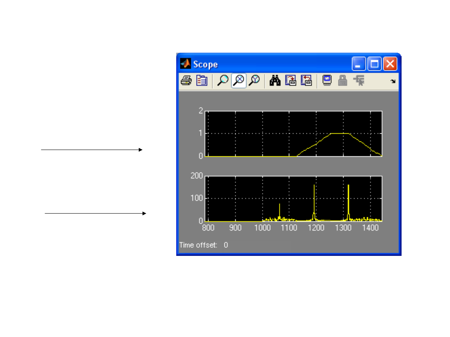
Compare the two (non dispersive channel):
y
r
yp
r
Autocorrelation of
received data
Crosscorrelation with
preamble

Synchronization with Dispersive Channel
Let L be the length of the channel impulse response
L
−
64
Channel impulse
response

In order to determine the starting point, compute the energy on a sliding window and
choose the point of maximum energy
][nr
yp
1
xcorr
][ny
][np
Σ
n
∑
−
=
−=
1
0
][][
M
k
yp
knrnc
][nc
][nr
yp
Maximum
energy
][nc
M=max length of
channel = length of CP
1+− Mn

][nr
yp
xcorr
][ny
][np
Σ
][nc
Impulse response
of channel
Example

Σ
][nc
Auto
correlation
Cross
correlation
][np
][ny
max

Autocorrelation (saw
previously)
Cross correlation
Sum
Detect
MAX

][nh
][nw
OFDM
TX
OFDM
RX
]0[
m
X
][kX
m
]1[ −NX
m
]0[
m
Y
][kY
m
]1[
−
NY
m
M
M
M
M
][kX
m
][][][][ kWkXkHkY
mm
+
=
][kH
][kW
m-th data block
⎪
⎪
⎩
⎪
⎪
⎨
⎧
Channel Estimation
Recall that, at the receiver, we need the frequency response of the channel:
Transmitted:
Received:
channel freq.
response

From the Preamble: at the beginning of the received packet. The transmitted signal in
the preamble is known at the receiver: after time synchronization, we take the FFT of
the received preamble
]0[Y
64 128 128
Received Preamble:
Estimated initial time
256 samples
L
FFT
L
]255[Y
][kY
255,...,0],[][][][
=
+
= kkWkXkHkY
p
255,...,0],[][][][
=
+
= kkWkXkHkY
p
Solve for using a Wiener Filter (due to noise):
22
*
|][|
][][
][
ˆ
wp
kX
kXkY
kH
preamble
σ
+
=
noise covariance
][kH
Problem: when we cannot compute the corresponding
frequency response
0][
=
kX
p
][kH
Fact: by definition,
jkX
p
±
±
=
1][
254,...,158,156
100,...,4,2
=
=
k
k
if
0][
=
kX
p
otherwise (ie DC, odd values,
frequency guards)

Two solutions:
1. Compute the channel estimate
22
*
|][|
][][
][
ˆ
wp
kX
kXkY
kH
preamble
σ
+
=
only for the frequencies k such that
0][
≠
kX
p
and interpolate for the other frequencies. This might not yield good results and the
channel estimate might be unreliable;
k
LL
known
interpolate

2. Recall the FFT and use the fact that we know the maximum length L of the
channel impulse response
][][2][][][
*
1
0
2
*
kXkWenhkXkY
p
L
n
n
N
jk
p
+
⎟
⎟
⎠
⎞
⎜
⎜
⎝
⎛
=
∑
−
=
−
π
][][][][ kWkXkHkY
p
+
=
Since the the preamble is such that either or
0|][|
=
kX
p
2|][| =kX
p
For the indices where we can write:
254,...,158,156
100,...,4,2
=
=
k
k
for
so that we have 100 equations and L=64 unknowns.
This is solved by a matrix multiplication
(
)
*
pinv
YXFh =
164
×
1100
×
2|][| =kX
p

Data in
Trigger when preamble is detected
Channel
Estimate out
Simulink Implementation
][ny
][kY
][
*
kX
p
][nh
][kH

Example:
Spectrum of
Received Signal
Estimated
Frequency
Response of
Channel
NOT TO
SCALE
As expected, it
does not match in
the Frequency
Guards

WiMax-2004 Demodulator
WiMax256.mdl
data
Ch.
Start after processing
preamble
Standard OFDM
Demod (256 carriers)
Error Correction
Decoding

Channel Tracking
In mobile applications, the channel changes and we need to track it.
IEEE802.16-2005 tracks the channel by embedding pilots within the data.
In the FUSC (Full Use of Sub Carriers) scheme, the pilots subcarriers are chosen
within the non-null subcarriers as
139
+
+
mk
with
[
]
2,1,03mod exsymbol_ind
=
=
m
⎪
⎪
⎩
⎪
⎪
⎨
⎧
=
=
=
=
=
128for 11,...,0
512for 47,...,0
1024for 95,...,0
2048for 191,...,0
FFT
FFT
FFT
FFT
N
N
N
N
k

nulls
DC
(null)
pilots
data
nulls
OFDM
Symbol
m
subcarrier
k
0
1
4
7
L

Expand the
Demodulator

Demodulator
Channel
tracking

Multiple Antenna Systems (MIMO)
TX
RX
M
M
T
N
R
N
Transmit
Antennas
Receive
Antennas
MM
RT
NN
×
Different paths
Two cases:
1. Array Gain: if all paths are strongly correlated to which other the SNR can be
increased by array processing;
2. Diversity Gain: if all paths are uncorrelated, the effect of channel fading can be
attenuated by diversity combining

Receive Diversity:
TX
RX
M
1=
T
N
R
N
Transmit
Antennas
Receive
Antennas
M
R
N
Different paths
s
1
y
R
N
y
⎥
⎥
⎥
⎦
⎤
⎢
⎢
⎢
⎣
⎡
+
⎥
⎥
⎥
⎦
⎤
⎢
⎢
⎢
⎣
⎡
=
⎥
⎥
⎥
⎦
⎤
⎢
⎢
⎢
⎣
⎡
RRR
N
S
NN
w
w
NsE
h
h
y
y
MMM
1
0
11
1
h
R
N
h
Noise PSD
Energy per
symbol

Assume we know the channels at the receiver. Then we can decode the signal as
∑∑∑
===
+==
RRR
N
i
ii
N
i
iS
N
i
ii
whNshEyhy
1
*
0
1
2
1
*
||
signal
noise
and the Signal to Nose Ratio
0
1
2
||
N
E
hSNR
S
N
i
i
R
⎟
⎟
⎠
⎞
⎜
⎜
⎝
⎛
=
∑
=

Now there are two possibilities:
1. Channels strongly correlated. Assume they are all the same for simplicity
hhhh
R
N
=
=
=
=
...
21
In the Wireless case the channels are random, therefore is a random variable
∑
=
R
N
i
i
h
1
2
||
Then
2
2
2
1
2
||||
χ
RR
N
i
i
NhNh
R
==
∑
=
and
()
0
2
2
0
2
2
1
||
N
E
N
N
E
hNSNR
S
R
S
R
⎟
⎠
⎞
⎜
⎝
⎛
==
χ
assuming
{
}
1||
2
=hE
{}
0
N
E
NSNREm
S
RSNR
==
{}
0
2
var
N
E
N
SNR
S
R
SNR
==
σ
better on average …
… but with deep fades!
From the properties of the Chi-Square distribution:
Define the coefficient of variation
2
1
var
==
SNR
SNR
m
σ
μ
In this case we say that there is no diversity.

Recall the Chi-Square distribution:
2
n
y
χ
=
22
2
2
1
...
n
xxxy +++=
...,)1,0( diirealNx
i
≈
1. Real Case. Let
Then
ny
nyE
2}var{
}{
=
=
with
2
2
2
1
n
y
χ
=
22
2
2
1
||...||||
n
xxxy +++=
...,)1,0( diigaussiancomplexCNjbax
iii
≈
+
=
2. Complex Case. Let
Then
ny
nyE
2
1
}var{
}{
=
=
with

2. Channels Completely Uncorrelated.
2
2
1
2
2
1
||
R
R
N
N
i
i
h
χ
=
∑
=
0
1
2
||
N
E
hSNR
S
N
i
i
R
⎟
⎟
⎠
⎞
⎜
⎜
⎝
⎛
=
∑
=
Since:
0
2
2
2
1
N
E
SNR
S
N
R
⎟
⎠
⎞
⎜
⎝
⎛
=
χ
with
{}
0
N
E
NSNRE
S
R
=
{}
0
2
var
N
E
N
SNR
S
R
=
R
SNR
SNR
N
m
2
1
var
==
σ
μ
Diversity of order
R
N

0 20 40 60 80 100 120 140 160 180 200
-25
-20
-15
-10
-5
0
5
10
15
Example: overall receiver gain with receiver diversity.
1
=
R
N
2
=
R
N
10
=
R
N

Transmitter Diversity
TX RX
M
T
N
1
=
R
N
Transmit
Antennas
Receive
Antennas
M
T
N
Different paths
s
y
1
h
R
N
h
wNsh
N
E
y
T
N
i
i
T
S
0
1
+
⎟
⎟
⎠
⎞
⎜
⎜
⎝
⎛
=
∑
=
Total energy equally distributed
on transmit antennas
Equivalent to one channel,
with no benefit.

However there is a gain if we use Space Time Coding.
Take the case of Transmitter diversity with two antennas
TX RX
][ny
1
h
2
h
][
1
nx
][
2
nx
Given two sequences
code them within the two antennas as follows
][],[
21
nsns
n212
+
n
1
s
2
s
*
2
s−
*
1
s
1
x
2
x
()
102211
2
]2[ wNshsh
E
ny
S
++=
()
20
*
12
*
21
2
]12[ wNshsh
E
ny
S
++−=+

This can be written as:
⎥
⎦
⎤
⎢
⎣
⎡
+
⎥
⎦
⎤
⎢
⎣
⎡
⎥
⎦
⎤
⎢
⎣
⎡
−
=
⎥
⎦
⎤
⎢
⎣
⎡
+
*
2
1
0
2
1
*
1
*
2
21
*
2
]12[
]2[
w
w
N
s
s
hh
hh
E
ny
ny
S
To decode, notice that
()
*
111
2
12
0
*
*
222
21
[2 ]
|| || || ||
[2 1]
2
S
z
sw
yn
hh
E
hNh
z
sw
yn
hh
⎛⎞
⎡⎤
⎡⎤ ⎡⎤ ⎡ ⎤
⎡⎤
==+
⎜⎟
⎢⎥
⎢⎥ ⎢⎥ ⎢ ⎥
⎢⎥
⎜⎟
+
−
⎣⎦
⎣⎦ ⎣⎦ ⎣ ⎦
⎣⎦
⎝⎠
%
%
Use a Wiener Filter to estimate “s”:
(
)
()
]12[]2[
ˆ
]12[]2[
ˆ
*
1
*
21
*
2
*
11
+−=
++=
nyhnyhKs
nyhnyhKs
S
S
ENhh
E
K
/2||||
/2
0
2
2
2
1
++
=
with

It is like having two independent channels
1
z
1
s
2
s
2
||||
2
h
E
S
2
||||
2
h
E
S
2
z
01
|| ||Nhw
%
0
2
2
||||
N
E
h
SNR
S
=
Apart from the factor ½, it has the same SNR as the receive diversity of order 2.
02
|| ||Nhw
%
2
4
2
2
2
1
2
2
1
||||||||
χ
=+= hhh
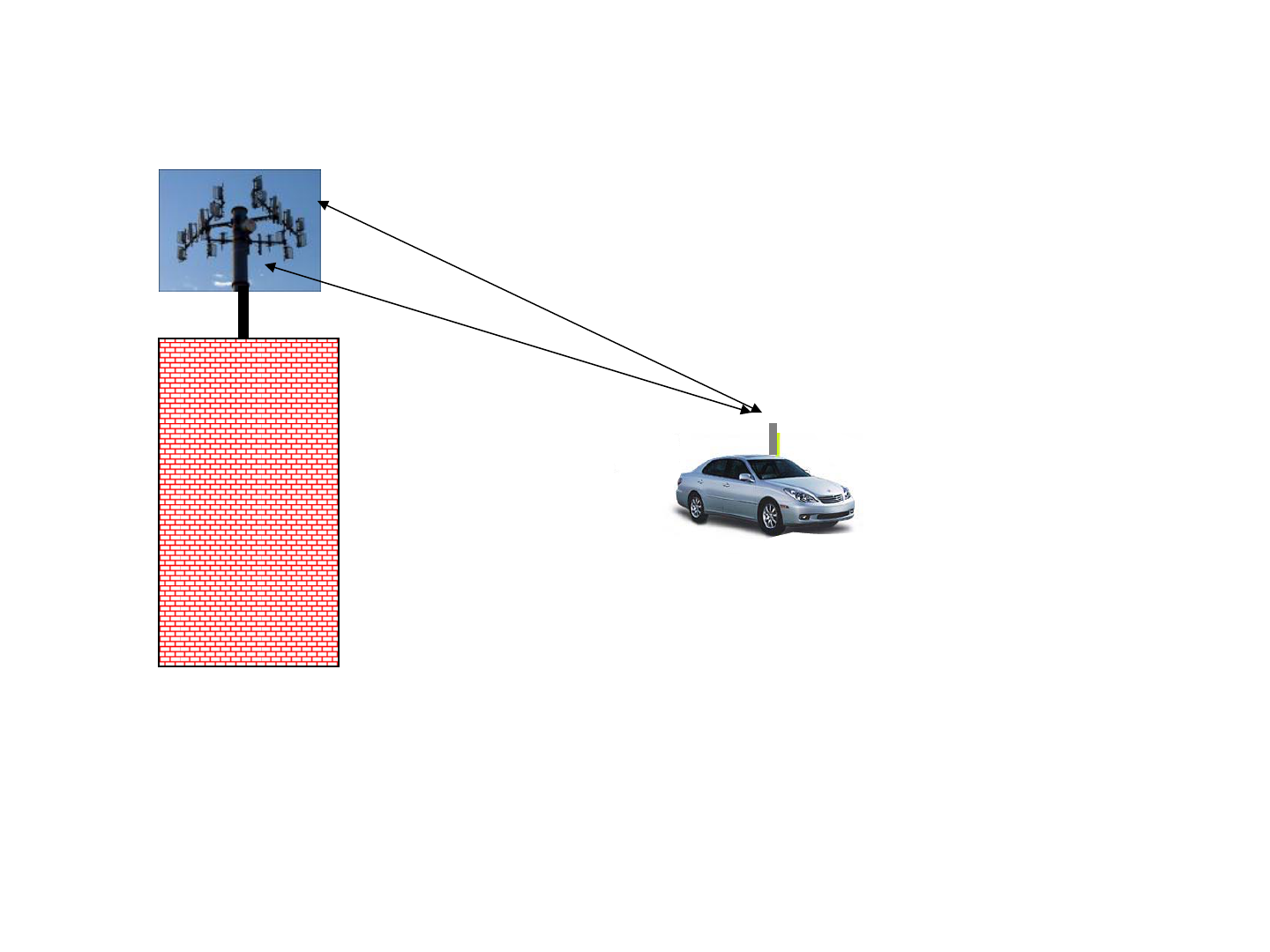
WiMax Implementation
1
h
2
h
Base Station
Subscriber
Station
Down Link (DL): BS -> SS Transmit Diversity
Uplink (UL): SS->BS Receive Diversity
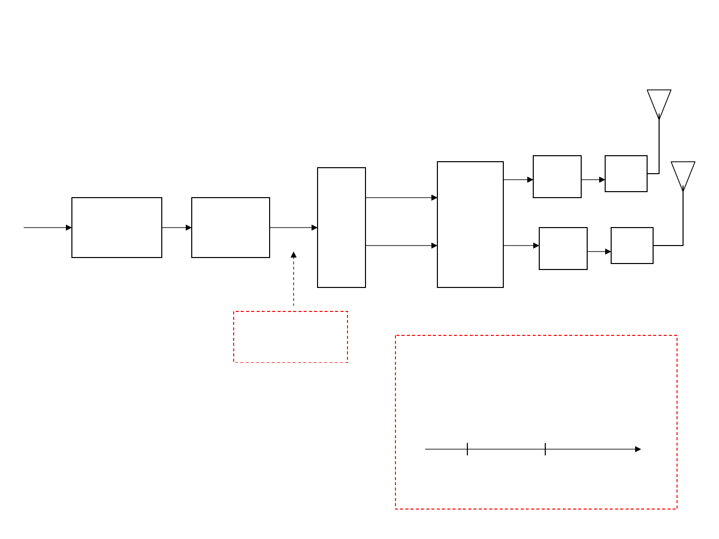
Down Link: Transmit Diversity
Use Alamouti Space Time Coding:
Error
Coding
Data in
M-QAM buffer
n
X
Block to be
transmitted
m
X
2
12
−m
X
STC
IFFT TX
IFFT TX
m2 12
+
m
m
X
2
12
−m
X
*
12 −
−
m
X
*
2
m
X
Space Time Coding
time
Transmitter:
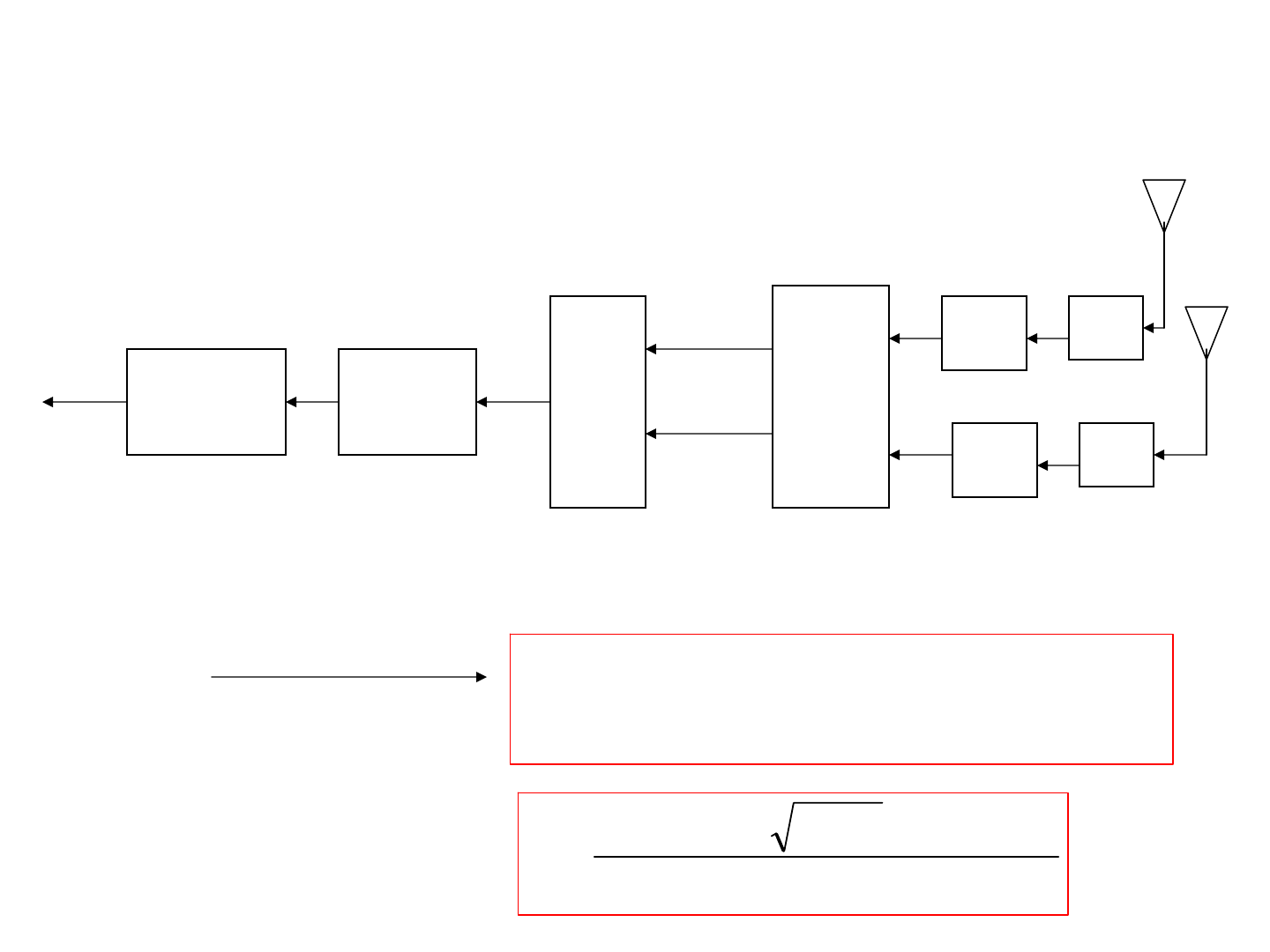
Error
Correction
Data out
M-QAM
Un-
buffer
n
X
m
X
2
12
−m
X
STD
FFT RX
FFT RX
Receiver:
m
Y
2
12
+m
Y
(
)
()
][][][][][
ˆ
][][][][][
ˆ
*
1212
*
212
*
1222
*
12
kYkHkYkHKkX
kYkHkYkHKkX
mmm
mmm
+−
+
−=
+=
S
S
ENkHkH
E
K
/2|][||][|
/2
0
2
2
2
1
++
=
with
Space Time Decoding:
For each subcarrier k
compute:

Preamble, Synchronization and Channel Estimation with
Transmit Diversity (DL)
The two antennas transmit two preambles at the same time, using different sets of
subcarriers
128
128
64
CP
L L
k
100− 100
−
0
128
128
128
64
CP
128
EVEN subcarriers
ODD subcarriers
][
0
np
][
1
np
++
+
-
n
0 319
time
frequency

Both preambles have a symmetry:
]128[][
]128[][
11
00
−−=
−=
npnp
npnp
319,...,128
=
n
][
0
nh
][
1
nh
][ny
][
0
np
][
1
np
received signal from
the two antennas
Problems:
• time synchronization
• estimation of both channels

One possibility: use symmetry of the preambles
][ny
128−
z
][*][2][
111
npnhny
=
+
+
+
−
][*][2][
000
npnhny
=
0
n
64 256
128
0
+
n
64 128
128
0
+
n
64 128
The two preambles can be easily separated

MIMO Channel Simulation
Take the general 2x2 channel
3
ϕ
j
e
4
ϕ
j
e
T
ρ
T
ρ
T
ρ
T
ρ
1
ϕ
j
e
2
ϕ
j
e
Rayleigh
Rayleigh
][
1
nx
][
2
nx
][
1
ny
][
2
ny
dBPPP
N
N
][
sec][
1
1
L
L
=
=
τ
τ
τ
10 ≤≤
T
ρ
10 ≤≤
R
ρ
Correlation at the receiver
Correlation at the transmitter

OFDM Transceiver
IFFT
M M
P/S
I
Q
LPF
LPF
MOD
BPF
MOD
BPF
I
F
F
CIF
F
F
−
Power
Amp
DAC
DAC
oscillator
BPF
DEM
BPF
FFT
M M
S/P
I
Q
LPF
LPF
DEM
ADC
ADC
I
F
F
CIF
F
F
−
oscillator
Low Noise
Amp
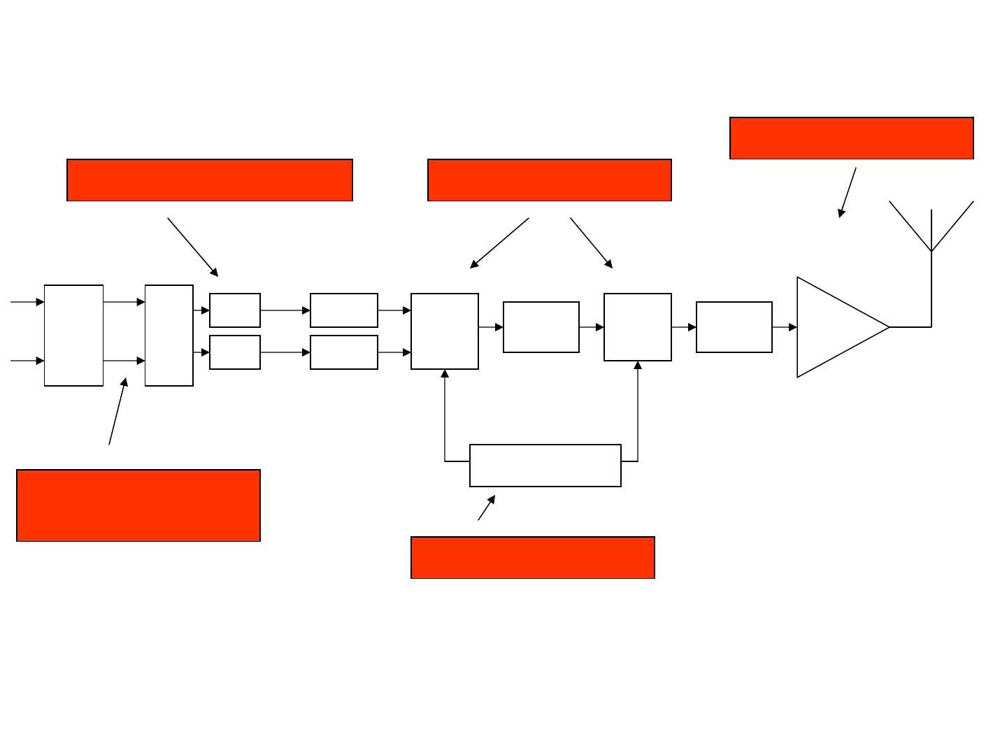
Problems!!!
IFFT
M M
P/S
I
Q
LPF
LPF
MOD
BPF
MOD
BPF
I
F
F
CIF
F
F
−
Power
Amp
DAC
DAC
oscillator
Quantization Errors I/Q Imbalance
Peak to Average
Power Ratio
Non Linearities
Frequency Drift

• Peak to Average Power Ratio (PAR)
A Single Carrier QPSK signal has a constant amplitude, since only the phase is
modulated.
A Multi Carrier OFDM signal has a random amplitude.
0 2 4 6 8 10 12
x 10
5
0
0.005
0.01
0.015
Pmax=0.014
Pave=2e-4
Pmax/Pave=66.88=18dB
Example: see an OFDM signal with 1024 subcarriers. Plot 1,000 OFDM
symbols

Effects:
• On the ADC
: larger number of bits to accommodate large dynamics
• On the Power Amplifier:
it has to be linear within a wider range
Remedies:
• the signal needs to be clipped to avoid saturating the amplifier
• the output power of the signal has to be reduced

Cause of large peaks:
OFDM signal is a sum of sinusoids. When all in phase, the sum can be large (peak
value) with respect to the average.
∑
−
=
=
1
0
2
][
1
][
N
k
njk
N
ekY
N
ny
π
Assume all subcarriers Y[k] are i.i.d.:
{} {}{}
2
1
0
2
2
2
|][|
1
|][|
1
|][| kYE
N
kYE
N
nyE
N
k
==
∑
−
=
Average Power:
Peak Power when all subcarriers are aligned:
{
}
2
2
||][|][| YYkYnyE ≤=
N
P
P
Ave
Peak
∝
It increases with the number of subcarriers

How bad is PAR?
Probability Distribution of PAR
{}
(
)
(
)
2.8
Pr 1 1
N
z
PAR z e
−
>=−−
fairly accurate for number of carriers
64N ≥
By the Central Limit Theorem the received signal is gaussian
The amplitude is Rayleigh distributed and the power is Chi-square.
Therefore we can compute the Cumulative Density Function analytically:
][ny

Notice:
1. The probability that PAR=N, the number of subcarriers, is almost zero;
2. The probability that PAR>4=12dB is of the order of
2 4 6 8 10 12 14
-7
-6
-5
-4
-3
-2
-1
0
z dB
()
)log
10
zPARP >
N=128,256,512,1024
5.35.4
1010
−−
−

Remedies:
1. Data randomizing
: if there is an error due to PAR, resend the data and most
likely it will be fine
2. Clipping
: easy thing to do, at the expenses of introducing errors
3. Coding
: potentially the best, but still not reliable solutions (not in the standard)
4. A number of iterative
techniques: too complex for real time implementation

ZOH
][nv
in
)(tv
out
QCL
η
DAC
][nv
in
)(tv
out
⇔
In the DAC there are two sources of errors:
• Quantization Error;
• Saturation error due to clipping
For a fixed number of bits, we need to compromise between two sources of
errors:
Effects of PAR on Digital to Analog
Converters (DAC)
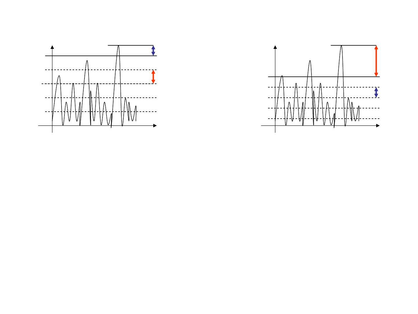
Compromise between Number of Bits in DAC and Clipping Level
min
V
MAX
V
min
V
MAX
V
Small clipping error, Large
Quantization Noise
Large clipping error, Small
Quantization Noise
t
t
We choose Clipping Level for best compromise between clipping error and
quantization noise.

ZOH
][nv
in
)(tv
out
QCL
η
()
2/3
8
2
2
1
11
2
)2(
212
μ
π
μ
μ
eSNR
SNR
SNRSNRSNR
CL
b
Q
CLQQCL
=
×
=
+=
−
−−
DAC
][nv
in
)(tv
out
⇔
/
CLIP
A
μ
σ
=
where
{
}
2
|][| nxE=
σ
Total SNR due to Q and CL:
SNR due to Q :
SNR due to CL :
b = number of bits per sample
ideal

/
CLIP
A
μ
σ
=
()SNR dB
8b
=
9b
=
10b
=
11b
=
12b
=
2 3 4 5 6 7 8
15
20
25
30
35
40
45
50
55
60
65
MAX around
/45
CLIP
A
μ
σ
=
=−
{
}
2
][4 nvEV
inMAX
≈
Choose max clipping value:
number of bits
See both combined:
We have seen that the probability that PAR>4=12dB is very small.

in
P
out
P
MAX
P
ave
P
Input
Back Off
(IBO)
()
p
p
x
xg
2
1
2
1
1
)(
+
=
)(tx
(
)
)()( txgty
=
g
p of the order of 3
Rapp’s model of a Power Amplifier:
Effects of PAR on Power Amplifiers

PAR
P
P
IBO
ave
MAX
>=
10
log10
10
10logPAR N
≤
Ideally you want the Input Back Off (IBO) to be larger than the PAR.
This can be excessive and very inefficient.
Example
: with N=256 carriers you need a IBO of
dBPARIBO 24256
=
=
=
to guarantee that the amplifier always operates in the linear region.

Remedies: Clipping
][nx
⎩
⎨
⎧
≤
>
=
∠
Anxnx
AnxAe
nx
nxj
CL
|][| if ][
|][| if
][
][
clip
A
|][| nx
|][][| nxnx
CL
−
time
time
FT
frequency
wide band noise

][
~
][][ nxnxnx
CL
−
=
A
|][| nx
time
i
n
][nx
clip Filter
∑
∑
−−≅
−−=
i
i
j
i
i
i
j
iW
nnweanx
nnweanwnxnx
i
i
][][
][][*][][
φ
φ
∑
−=
i
i
j
i
nneanx
i
][][
~
δ
φ
)(FX
)(
~
FX
F
F
)(FW

It has two effects:
1. Additive Noise in the demodulated subcarriers
2. It generates out of band noise, so we need to add a Low Pass Filter
The latter is not allowed, since it interferes with neighboring channels.

Example:
See one of OFDM symbol with the following parameters (this is not random but
chosen with high PAR):
FFT length N=256
Data Carriers: Nused=200
Modulation: 4QAM
0 50 100 150 200 250 300
0
0.05
0.1
0.15
0.2
0.25
0.3
0.35
0.4
|][| nx
n
Large peak value

Clip it to 5dB (no filtering):
See the Frequency Spectrum:
S
F
F
f =
0
2
1
2
1
−
N
Nused 2/
N
Nused 2/
−
data
nullsnulls
-0.5 -0.4 -0.3 -0.2 -0.1 0 0.1 0.2 0.3 0.4 0.5
-25
-20
-15
-10
-5
0
5
unfiltered clipped signal
Large values in
the freq. guards

-15 -10 -5 0 5 10 15
-0.2
0
0.2
0.4
0.6
0.8
1
1.2
window
-0.5 -0.4 -0.3 -0.2 -0.1 0 0.1 0.2 0.3 0.4 0.5
-60
-50
-40
-30
-20
-10
0
10
FT of window
Choose a filter with this characteristics:
f
5.0
stop
f
pass
f
(
)
NNusedf
pass
2/
=
2/1
<
<
stoppass
ff
In matlab: use firpm
h=firpm(M, [0,fpass,fstop,0.5]*2, [1,1,0,0]);
filter order, say M=40
1
][nh
|)(| fH

-0.5 -0.4 -0.3 -0.2 -0.1 0 0.1 0.2 0.3 0.4 0.5
-80
-70
-60
-50
-40
-30
-20
-10
0
10
filtered and unfiltered clipped signal
F/Fs
dB
Clipped and Filtered:
Clipped only (no filter)
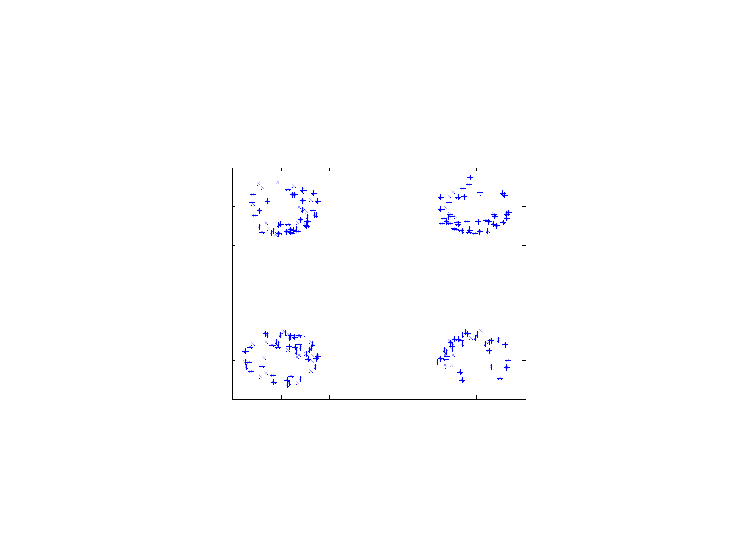
Negative effect on data!!!
-1.5 -1 -0.5 0 0.5 1 1.5
-1.5
-1
-0.5
0
0.5
1
1.5

Peak Cancellation
Detect and Cancel the peak to reduce out of band noise.
Detect
peak
Generate
impulses
LPF
+
-
t
t
0
t
0
t
(
)
)()(
0
)(
0
0
ttAetx
txj
−−
∠
δ
A
|)(| tx
(
)
)()(
0
)(
0
0
ttgAetx
txj
−−
∠
It spreads the error to
neighboring values.
Larger in band noise

Effects:
• The LPF completely controls the out of band noise. It can be completely eliminated;
• It reduced PAR and therefore the Input Back Off.
• It causes an increase of in band noise and therefore a higher BER.

Effect of I/Q Imbalance
Ideally the received signal is of the form
][][][][
1
0
2
njynyekYny
QI
N
k
njk
N
+==
∑
−
=
π
In practice the I and Q components have different gains, as
()
[] [] []
(1 ) [ ] (1 ) [ ]
Q
I
j
j
II QQ
jj j
IQ
yn Ae y n jAe y n
A
eeynjeyn
ϕ
ϕ
ϕε ε
δδ
−
=+
=+ +−
2
2
QI
QI
AA
A
ϕϕ
ϕ
+
=
+
=
with
QI
QI
QI
QI
AA
AA
ϕϕ
ϕϕ
ε
δ
+
−
=
+
−
=

The two parameters express the magnitude and phase of the I/Q imbalance.
Assume them small:
εδεδδ
ε
jje
j
++≅++≅+ 1)1)(1()1(
(1 ) (1 )(1 ) 1
j
e
jj
ε
δ
δεδε
−
−≅−−≅−−
(
)
(
)
*
[] [] []
j
y
nAe
y
n
jy
n
ϕ
δε
=++
After a bit of algebra:
2
1
0
[] []
N
N
j
kn
k
yn Yke
π
−
=
=
∑
Substitute:
ε
δ
,
()
22
2
11
*
00
1
*
0
[] [] ( ) []
[ ] ( ) [ ]
NN
N
NN
j
kn j n
j
k
N
jk n
j
k
yn Ae Yke j Y e
Ae Y k j Y N k e
ππ
π
ϕ
ϕ
δε
δε
−−
−
==
−
=
⎛⎞
=++
⎜⎟
⎝⎠
⎛⎞
=++−
⎜⎟
⎝⎠
∑∑
∑
l
l
l
to obtain:

The effect is subcarrier N-k leaking into subcarrier k
kN
−
k
It is as having extra noise added to the signal:
][ny
noise
I/Q Imbalance
L
ε
δ
j
+
][kY []YN k
−

The factor is called Negative Frequency Rejection and it can be
modeled as covariance of additive noise.
||
ε
δ
j+
][ny
noise
I/Q Imbalance
][
1
nw
][
2
nw
][ny
(
)
10
21
101log101log10log10log10
2
1
2
2
2
1
2
2
2
2
1
2
SNRSNR
yy
−
+−=
⎟
⎟
⎠
⎞
⎜
⎜
⎝
⎛
+−=−
+
σ
σ
σ
σ
σσ
σ
2
2
log10
i
y
i
SNR
σ
σ
=
Define:
Implementation Loss:

Example: let
dBSNR
dBSNR
IQ
noise
35
20
=
=
Implementation Loss
(
)
135.0101log10
10
3520
−=+−
−
Total SNR:
dBILSNR
noise
65.18135.020
=
−
=
+

Frequency Synchronization
• Drifts and errors in the oscillator frequencies cause a frequency offset, like a doppler
shift;
• This causes loss of subcarriers orthogonality and Inter Carrier Interference (ICI).
• The effect of ICI can be modeled as additive noise, which can be quantified

Fact: to maintain satisfactory SNR we need to limit the frequency offset
to
%4
/
||
≤
Δ
=
NF
F
S
ε
0 0.02 0.04 0.06 0.08 0.1
5
10
15
20
25
30
epsilon
dB
SNR

• Frequency Synchronization from Long Preamble.
0
n
CP
n
][nx
P
x
P
x
If there is a frequency offset (due to oscillator drifts or doppler shift) the
received signal has an extra phase term
2
0
[] []
j
fn
yn y ne
π
Δ
=
with the digital frequency offset. Take the two received parts of the long
preamble:
fΔ
(
)
()
2
10 1
2( )
20 2
[] [] []
[] [] []
jfn
jfnN
yn yne wn
y
n
y
ne w n
πα
πα
Δ+
Δ++
=+
=+
1,...,0
−
=
Nn
128
=
N 128=N

Comparing the two in vector form:
2
21
jfN
yy
ew
π
Δ
=+
[]
T
iii
Nyyy ]1[]0[ −= Lwhere
Then:
*22*
12 1 1
|| ||
TjfNT
yy y e yw
π
Δ
=+
which yields the estimate of the frequency offset
{
}
{}
*
12
*
12
Im
1
arctan
2
Re
T
T
yy
f
N
yy
π
⎛⎞
Δ=
⎜⎟
⎜⎟
⎝⎠
Since, then the frequency offset has to be at the most
1
2
f
N
Δ<
π
<|arctan|
with N being the FFT length.
