
BMG LABTECH
Omega Software Manual - Part III: MARS Data Analysis
1/81
0415F0045A
27.07.2017
Part III: MARS Data Analysis
Version 3.31

Omega Software Manual - Part III: MARS Data Analysis
BMG LABTECH
27.07.2017
0415F0045A
2/81
This manual was designed to guide users through the software features.
Although these instructions were carefully written and checked, we cannot accept responsibility for problems encountered when using
this manual. Suggestions for improving this manual will be gratefully accepted.
BMG LABTECH reserves the right to change or update this manual at any time. The Revision-Number is stated at the bottom of every
page.
Copyright © 2017 BMG LABTECH. All rights reserved. All BMG LABTECH brand and product names are trademarks of BMG LABTECH. Other brand and
product names are trademarks or registered trademarks of their respective holders.

BMG LABTECH
Omega Software Manual - Part III: MARS Data Analysis
3/81
0415F0045A
27.07.2017
TABLE OF CONTENT
1 Overview 5
1.1 Main Screen of MARS 5
1.2 Login 5
1.2.1 Login at Start Up 5
1.2.2 Changing the User 5
1.3 Multiple Installations 5
1.4 Run MARS in automatic mode 5
2 Manage Test runs 6
2.1 Different Table Views 7
2.1.1 Microplates Table 7
2.1.2 BMG LVis Micro Drop plates Table 7
2.2 Group and Filter Test Runs 7
2.2.1 Sorting the Table 7
2.2.2 Grouping the Table 8
2.2.3 Change the Position of a Column 8
2.2.4 Filtering the Table 8
2.3 Import / Export Test Runs 8
2.3.1 Import Test Runs 8
2.3.2 Export Test Runs 9
2.4 Merging Test Runs 9
2.4.1 What Means Merging Test Runs 9
2.4.2 Merge Cycles / Intervals 9
2.4.3 Merge Wavelength 9
2.4.4 Merge Wells 10
2.5 Test Run Settings 10
3 Explore Data 10
3.1 Navigation Tree 11
3.1.1 Using the Tree 11
3.1.2 Detailed Information on the Selected Node 15
3.2 Content Filter Tree 15
3.3 Microplate View 15
3.3.1 View Modes 16
3.3.2 Selecting Wells 17
3.3.3 Details of a Well 18
3.3.4 Zooming 18
3.3.5 Exclude Wells 18
3.3.6 Microplate Bar Chart 18
3.3.7 BMG LVis Micro Drop Plates 19
3.4 Table View 19
3.5 Well Scan Area Statistic Table 20
3.6 Common Chart Functions 20
3.6.1 Chart Axes and Curves 21
3.6.2 Changing chart legend entries 21
3.6.3 Crosshair 21
3.6.4 Chart Popup Menu 21
3.6.5 Zooming 22
3.6.6 Chart Comments 22
3.7 Change Settings of a Chart Axis 22
3.8 Change Chart Curve Settings 23
3.9 Chart Title Settings 24
3.10 Chart Legend Settings 24
3.11 Signal Curve 24
3.11.1 Range Functions in the Chart 25
3.11.2 Show Injection Markers 25
3.11.3 Show Error Bars 25
3.12 Spectrum Curve 25
3.12.1 Adding, Changing or Removing Wavelengths 26
3.12.2 Change the Lambda Value of a Discrete
Wavelength 27
3.12.3 Deleting a Discrete Wavelength 27
3.12.4 Spectra and Kinetics 27
3.12.5 Combined excitation and emission spectra 27
3.13 Standard Curve 28
3.13.1 Error Bars, Replicates of Standards, Confidence
Band and Recalculated Values 28
3.13.2 Fit Result Window 29
3.14 Enzyme Kinetic Fit Curves 30
3.14.1 Error Bars 30
3.14.2 Fit Result Window 30
3.15 Binding Kinetics Fit Curves 30
3.15.1 Fit Result Window 31
3.16 Protocol Information 31
3.17 21 CFR part 11 31
3.18 Measurement Notifications 32
3.19 Color Settings 32
3.19.1 Two Colors (Good, Bad) 32
3.19.2 Three Colors (Range) 32
3.19.3 Color Gradient 32
3.20 Printing Your Data 32
3.20.1 Preview 33
3.20.2 Define Page Margins 34
3.20.3 Define Print Header and Footer 34
3.20.4 Quick Print Function 35
3.20.5 Print Settings 35
3.21 Export Data 36
3.21.1 Export Displayed Data 36
3.21.2 Exporting Fit Results 37
3.21.3 Define an Excel Report 37
3.22 Well Scanning Data 37
3.22.1 Detailed View of Well Scanning Data for a
Selected Well 37
3.23 View Microplate Layout 40
3.24 Settings 40
3.24.1 MARS Settings 40
3.24.2 Excel Export Settings 41
3.24.3 File Export Settings 41
3.24.4 Spectrum Display Settings 42
3.24.5 Number Format Settings 43
3.24.6 Number Format Settings for Data Nodes and
Chart Axes 44
3.25 Outlier Detection 45
4 Perform Calculations 45
4.1 Ranges 46
4.1.1 Predefined Ranges 46
4.1.2 Individual Ranges 46
4.1.3 Define a Range 46
4.2 Variables 47
4.2.1 Define and Use Variables 47
4.2.2 Manage Variables 48
4.2.3 Select a Variable 49
4.3 Calculations 50
4.4 Corrections 51
4.4.1 Content Based Corrections 51

Omega Software Manual - Part III: MARS Data Analysis
BMG LABTECH
27.07.2017
0415F0045A
4/81
4.4.2 Blank Corrections 51
4.4.3 Negative Control Corrections 51
4.4.4 Baseline Corrections 52
4.5 Statistics 52
4.6 FP and TR-FRET Calculations 52
4.6.1 FP Calculations 53
4.6.2 TR-FRET Calculations 53
4.7 Curve Smoothing 53
4.7.1 Preview of the smoothed curve 54
4.8 Kinetic Calculations 54
4.9 Kinetic Fit Calculations 55
4.10 Standard Calculations 56
4.10.1 Fit Result 58
4.11 Concentration Calculations 59
4.12 Data Calculations 59
4.13 Validations 59
4.14 Assay Quality 60
4.15 User Defined Formula 61
4.15.1 Enter a formula 61
4.15.2 Export and Import a Formula 62
4.16 Enzyme Kinetic Calculations 63
4.16.1 Define Enzyme Dilution Factor(s) and Extinction
Coefficient(s) 63
4.16.2 Consider zero concentration reaction 64
4.16.3 Calculation Result 64
4.16.4 How to Perform an Enzyme Kinetic Experiment64
4.17 Curve Scaling 65
4.18 Spectrum Calculations 66
4.18.1 Extended parameters 67
4.18.2 Preview the smoothed curves 67
4.19 Statistic over Wells 67
4.20 Well Scan Statistics 67
4.21 Standard Calculation Wizard 68
4.21.1 When Can You Use the Wizard? 68
4.21.2 How the Wizard Works 68
4.22 ORAC Evaluation 69
4.22.1 Changing the Layout for ORAC Test Runs 69
4.22.2 ORAC Templates 69
4.22.3 Optimized Settings for ORAC Measurements 70
4.22.4 Trolox Equivalents (TE Values) 70
4.23 Robust Statistics 70
4.24 Curve Analysis 70
4.25 Binding Kinetics Calculations 71
4.25.1 Calculation Result 71
4.26 User defined fit formulas 71
4.27 Integration Time Wizard 71
5 Using Templates 72
5.1 Why Assign Templates to Protocols? 72
5.2 Manage Templates 73
5.2.1 List of Templates 73
5.2.2 Change Template Name 73
5.2.3 Assign Protocols to Templates 73
5.2.4 Removing Assigned Protocols From the
Template 74
5.2.5 Edit Parameters 74
5.2.6 Export and Import Templates 74
5.2.7 Delete Templates 74
5.3 Create a Template 74
5.4 Assigning Templates 75
5.4.1 Assign a Template to a Test Run 75
5.4.2 Assign a Template to a Protocol 75
5.5 Template Buttons 76
5.5.1 Templates Button 76
5.5.2 Add a User Template Button 76
5.5.3 Changing and Deleting User Template Buttons76
5.5.4 Manage Template Buttons 77
5.6 Transfer of Standard Fit Results 77
6 Test Run Layout 77
6.1 Changing Layout 77
6.1.1 Changing Plate IDs 78
6.1.2 Changing Layout Contents 78
6.1.3 Changing Concentrations, Dilutions and Sample
IDs 79
6.1.4 Changing Path Length Correction Settings 79
6.1.5 Changing Crosstalk Correction Settings 79
6.2 Manage Layouts 79
6.2.1 Assign a Saved Layout to a Test Run 80
6.2.2 Create and Edit Saved Layouts 80
6.2.3 Delete Layouts 80
6.2.4 Export and Import Layouts 80
7 Sign a Test Run 80
8 Support 81

BMG LABTECH
Omega Software Manual - Part III: MARS Data Analysis
5/81
0415F0045A
27.07.2017
1 Overview
1.1 Main Screen of MARS
After starting MARS, either from the control software or directly,
you will see a window with all available test runs (see chapter 2:
Manage Test Runs) of the logged in user (chapter 1.2 Login).
After selecting a test run and opening it, the data of the test run
will be available in the main window as shown below (this
picture was taken from a test run, measured with a CLARIOstar
with a build in monochromator and spectrometer):
The window is divided in two areas: The navigation tree on the
left side and the working area on the right side. The working area
displays your data in different ways, providing several pages
which you can access by clicking on the relevant tabs on the top
of the working area, e.g. Microplate View (the default page),
Table View, Spectrum, Standard Curve, etc. How data is displayed
in each page is explained in detail in the chapter 3: Explore Data.
The Ribbon with its task oriented tabs and groups gains you
access to all available task.
The status bar at the bottom of the screen shows the reader
series used to generate the data and the details of the user
logged in with the data path showing where the data is stored.
The status icon on the right side of the status bar shows if the
application is busy (red) or ready to accept user activities (green).
To check the version numbers of the software and the modules
used, click the File tab and then click Info. These version numbers
are needed when completing a technical support request.
1.2 Login
1.2.1 Login at Start Up
When starting MARS from the control software screen you do
not need to select a login user again. The software automatically
starts with the same user as used in the control software. If more
than one reader is installed on the computer, or if more than one
copy of the software is needed then please read the chapter 1.3:
Multiple Installations for more details.
If starting MARS without having the control software running,
you will get the same login window as if you had started the
control software. Enter the user name and the correct password
to log into the desired user.
If a user with the limited rights is used, some of the functions are
not available in MARS.
More details about the functions of the login window can be
found in the help of the control software or by pressing the F1
key on the keyboard, when the login window is shown.
1.2.2 Changing the User
To change to a new user account in MARS you can either click on
the status bar showing the current user or by clicking Change
User in the Test Runs group on the Home tab of the
Ribbon. Then the login window appears and you can log into the
desired user.
1.3 Multiple Installations
It is possible to install the control software part of the reader
more than once. For more details on how to do this see chapter
2 of software manual part I: Installation.
For each installation (called instances) of the control part there is
a corresponding instance of MARS. Starting MARS from the
control software automatically selects the same instance.
Beside instances you can start MARS more than once even with
the same user if you start it directly and not from the control
software screen.
1.4 Run MARS in automatic mode
It is possible to run MARS in an automatic mode. This mode can
be used to generate automatically character separated value
(CSV) text files (see chapter 3.21: Export Data) containing e.g. the
result of a calculation (like concentration calculations based on a
standards fit).
What happens exactly, when MARS runs in automatic mode?
MARS watches the test run data base.
Whenever a new test run was generated with the BMG
Labtech control software, this new test run will be opened in
background.
If a template is associated to the protocol of the test run, this
template is applied and the defined calculations will be
performed (see chapter 5: Using Templates).
A CSV file based on the table view contents is generated then
(the contents of the table view must be defined in the
template!).
The test run will be closed automatically and MARS waits for
the next new test run.
MARS can be started in the automatic mode by calling it with the
following parameters:
First Parameter
Reader Short ID (see Reader Short ID table below)
Second Parameter
Username
Third Parameter
User data directory (enclosed in " if the path
contains spaces)
Fourth Parameter
-3
Note: You can also call MARS only with the parameter -3 to
run it in automatic mode. You will be asked for the
used reader (if more than one is installed on the
computer) and the log-in dialog will be shown to select
the user.
Reader Short ID table: the Reader Short ID is an ID that identifies
the used reader to create the test run:
Reader Series
Short ID
CLARIOstar
CL
PHERAstar FS, FSX and PHERAstar Plus
PH
SPECTROstar Nano
SP
Omega
OM

Omega Software Manual - Part III: MARS Data Analysis
BMG LABTECH
27.07.2017
0415F0045A
6/81
Example:
If the reader is a CLARIOstar, the software was installed into the
default directory (c:\program files (x86)\bmg), the BMG User is
USER and the user data directory is the default directory
(c:\program files (x86)\bmg\CLARIOstar\User) then MARS must
be called like:
"c:\program files (x86)\bmg\mars\mars" CL
USER "c:\program files
(x86)\bmg\CLARIOstar\User" -3
You can perform this call manually if you open the Run... menu in
the Windows START menu and enter the call like in the example
above.
For an automatic starting of MARS you can insert this call in any
batch or script tool that allows calling other programs (like
windows batch files or BMG LABTECH's script language).
Note: If MARS was started in automatic mode, no window is
opened. You can only see the program item in the
notification area of the task bar. If you click on the item
the following window opens:
To close MARS, press the right mouse button over the program
item and select the Close menu or click on the item and press the
Close Application button.
To see and change the settings for the generated ASCII file, click
on the Settings... button to open the file export settings window
(see chapter 3.24.3: File Export Settings).
The status line of the AutoMode window shows if a valid
connection to the data base succeeded. Click Show Log to see a
detailed list of the performed steps and occurred events during
the automatic mode.
Click the Change to normal mode... button to stop the automatic
mode and start MARS in normal mode.
2 Manage Test runs
The Manage Test Runs window shows you all available test runs
of the current user.
You can reach the Manage Test Runs window by clicking Open in
the Test Runs group on the Home tab of the Ribbon, or click
Open in the File menu.
Note: This window opens automatically when you open
MARS or change the user, but not if you select Open
Last Test Run in the control software.
Note: The displayed window shows also a menu item above
the table for recent test runs and LVis plates. The LVis
tab is only visible, if test runs measured with the LVis
Mirco Drop plate are in the test run data base. To
change the displayed table, click on the appropriate
menu item.
Select a test run in the table by clicking on it with the mouse.
More than one test run can be selected by holding down the Ctrl-
Key whilst highlighting the desired test runs with the mouse and
clicking on them.
The test run window comes with several possibilities to sort,
arrange and filter your test runs. This is explained in detail in the
chapter 2.2: Group and Filter Test Runs.
The window provides you the following functions:
Opens all selected test runs and creates a node for each in the
navigation tree
Creates a copy of the selected test runs (creating a copy flag
indicated by a C in the state column)
Deletes all selected test runs.
Export the selected test runs (for more details see the chapter
2.3: Import / Export Test Runs).
Import one or more test runs (for more details see the chapter
2.3: Import / Export Test Runs).
Merge test runs. Learn more about merging test runs in the
chapter 2.4: Merging Test Runs
These functions (except the merge functions) are also available
on the popup menu of the window. You can open the popup
menu by pressing the right mouse button. The popup menu
contains three further menu entries:
Reset Test Run Settings and Changed Layout: Select this menu
entry to reset the settings and changed layout of the selected
test run(s). See chapter 2.5: Test Run Settings and 6.1: Changing
Layout.

BMG LABTECH
Omega Software Manual - Part III: MARS Data Analysis
7/81
0415F0045A
27.07.2017
Assign Layout: Select this menu entry to assign a saved layout to
the test run. See chapter 6.2.1: Assign a Saved Layout to a Test
Run.
Export Multiple ASCII files...: Select this menu entry to export
the selected test runs into ASCII (CSV) files. You will be asked
where to save the generated files. Standard file export settings
will be used like in the MARS auto mode.
To search a specific test run, you can press CTRL+F Key and enter
the text to search. The test run list will then be filtered displaying
only these test runs containing the entered text in one of its
columns.
If you open a test run created with a quick start protocol the first
time, you will see following dialog, to decide, whether to change
the well content information of the test run directly or to open
the test run normally:
Note: The user can change the order of the columns so they
may not appear in the same order as described (see
also chapter 2.2: Group and Filter Test Runs).
All tables (microplates, LVis) contain the following columns:
State
The state field describes the history of a test run. The available
states are defined below:
layout changed:
The layout of the test run has been changed after the
measurement.
plate IDs changed:
The plate IDs of the test run has been changed after the
measurement.
old:
The test run has been imported from an old data base, meaning
that no validation checks have been made in its history.
copied:
The test run is a copy of another test run.
merged:
The test run was generated by merging at least two test runs
together.
manipulated:
Manipulations have been detected since the generation of the
test run (manipulations done outside the evaluation software).
Manipulated test runs are shown in read in the test run list.
If the state field is empty, the test run is still in its original state.
Signed
Indicates if the test run is signed ('yes') or not (empty). It is not
possible to save further changes to this test run. See chapter 2.5:
Test Run Settings.
Test Name
The test name is listed as it is defined in the test protocol.
Date and Time
The date and time that the measurement took place.
Test ID
The unique number of the test run.
2.1 Different Table Views
2.1.1 Microplates Table
In addition to the common columns, the table with the
microplate measurements contains the following columns:
ID 1 / ID 2 / ID 3
These are the plate identifiers that were created before the
measurement.
Measurement Method
The measured method (e.g. absorbance, fluorescence...)
# Wells
The plate format (number of wells) of the microplate.
Protocol Comment
The comment of the test run protocol entered with the control
software.
Plate
The name of the used microplate.
2.1.2 BMG LVis Micro Drop plates Table
The BMG LVis Micro Drop plates table shows the same columns
as the Microplate table without the #Wells and the Plate
column.
2.2 Group and Filter Test Runs
The test run’s table provides powerful functions to help order
the stored test runs. The user can sort, group, use filtering and
change the order of columns to help find data and to achieve
their most useful view of the test run list.
If you change the settings of the test run table to your needs,
MARS memorizes the settings when you close the software and
will restore them when you open it again.
2.2.1 Sorting the Table
The table can be easily sorted by clicking on the column you
want to sort by. By clicking once on a column header the list will
be sorted in that column. This is indicated by a little arrow in
the column header. Clicking on the column header a second
time, will sort the list in a descending order by that column ( ).
It is possible to create a hierarchic sorting list, using more than
one column. Just select the main column in the list to sort by and
sort it as described above. To select the second sorting
parameter press and hold the Shift-Key on the keyboard, click on
the second column header you want as a next sort key and so on
with each new sort key.

Omega Software Manual - Part III: MARS Data Analysis
BMG LABTECH
27.07.2017
0415F0045A
8/81
2.2.2 Grouping the Table
In the window above you see a grouped table. The grouping
column is the Measurement Method column. As you see, the
table contains blocks for each Measurement Method in the list.
You can expand or close each block by clicking on the + or -
button before each block header.
Grouping helps in ordering your test runs and makes finding a
specific test run easy.
How to Group the List
The list can be grouped using the mouse. Move the mouse cursor
to the header of the column you want to use as a group criterion.
Click the left mouse button and keep it pressed, then move the
mouse cursor and highlighted column header to the gray area
above the list releasing the left mouse button when the cursor is
over the area, the data will then be sorted by the data in that
column.
As with the hierarchic sorting you can also group hierarchically
by selecting another column to drag to the group area.
2.2.3 Change the Position of a Column
If the default order of the columns is not suitable, you can
change the position of each column manually. Click on the
column header you want to move, and keep the mouse button
down whilst dragging the column to the new position. When a
position is reached where you can drop the column two green
arrows are displayed, the column can then be dropped into one
of these positions.
2.2.4 Filtering the Table
You can filter your list by nearly any filter criterion. The easiest
way of defining a filter is to click on the small down arrow of the
column header which appears if you move the mouse cursor
over the header. A list with the whole content of the column will
then be displayed:
Select one or more contents by clicking the check box before the
content title. To reset the filter for a single content just click the
check box again. To reset the whole filter, just select the ‘All’ list
entry from the drop down menu.
When a filter is defined, this is indicated by a new line which
appears at the top of the list:
There the filter can be deleted by clicking the red button with the
cross (x). If you want to discard the filter temporarily but leave
the definition for later use, just deselect the check-box before
the filter description by clicking on it, and to restore the filter
again just click again in the check box.
It is possible to further customize the filter. Press the Custom list
entry in the drop down menu to open the customize window. Try
out this function to learn how powerful this is.
Searching in the Table
To locate information within the table, you can use the search
function. Press the magnifier button at the top right corner or
CTRL+F to open the search entry field at the bottom of the table.
Enter the text to search and press Find. The list will filter records,
displaying only those that contain the entered search string (the
search is case-insensitive).
Extended Search Syntax
The following specifiers and wildcards can be used to narrow
search results:
The "+" specifier. Preceding a condition with this specifier causes
the table to display only records that match this condition. The
"+" specifier implements the logical AND operator. There should
be no space character between the "+" sign and the condition.
The "–" specifier. Preceding a condition with "–" excludes
records that match this condition from search results. There
should be no space between the "–" sign and the condition.
The percent (“%”) wildcard. This wildcard substitutes any
number of characters in a condition.
The underscore (“_”) wildcard. This wildcard represents any
single character in a condition.
For instance, applying the 'fluorescence TRF +9902 +EV –lin –
copied' search string makes the grid display only records that
include 'fluorescence ' or 'TRF ' with '9902' and 'EV ' in any cell,
and do not include either 'lin' or 'copied'.
2.3 Import / Export Test Runs
2.3.1 Import Test Runs
Using the import function you can import test runs. Click on the
Import button in the menu on the manage test runs window and
a standard file window opens where you can select a file with the
test runs you want to import into the current users data.
Imported test runs will be added to the test run list and marked.

BMG LABTECH
Omega Software Manual - Part III: MARS Data Analysis
9/81
0415F0045A
27.07.2017
Note: It is allowed to import test runs, generated with
different reader families. Because of technical reasons,
not all test runs are compatible.
Note: Test runs generated with a newer version of the same
reader family software cannot be imported if data base
format has changed.
If you have installed the newer BMG control software you can
also use drag and drop to import test run files (*.ruc). Select the
file with the test run in the Windows Explorer, hold down the left
mouse button and move the mouse over the manage test runs
window. Leave the mouse button and the test run(s) in the *.ruc
file will be imported.
2.3.2 Export Test Runs
You can export one or more test runs as one file to exchange it
between users.
Note: If making a support request regarding the test run(s) it
is useful to include exported data that demonstrates
the problems experienced as this can help in finding
and solving the problem.
If the manage test runs window is open, just select the test
run(s) you want to export in the list and click on the Export
button in the menu on the top of the window.
If you want to export only the currently opened and active test
run (the one which is selected in the navigation tree), click Export
in the Test Runs group on the Home tab of the Ribbon or click the
Export item in the File menu:
A standard file window will appear where a file destination can
be selected to save the exported test runs. Define a name for the
file (or accept the proposed one) and press the Save button. The
extension of the file name will be added automatically and is
always .RUC. Please do not change the extension manually as
this will mean that the created file will not be recognized by the
software when trying to re-import the file.
2.4 Merging Test Runs
2.4.1 What Means Merging Test Runs
The merging test runs function can be used to add the data of
one test run to another test run, resulting in one new test run
containing the data of both. There are three ways to merge test
runs together:
The kinetic cycles/intervals of two test runs can be merged
so that the new number of cycles/intervals is the sum of the
number of cycles/intervals of each.
The wavelengths of two or more test runs can also be
merged so that the number of wavelengths in the merged
test run is the sum of the number of wavelengths of each.
The wells of two test runs if each well is measured in only
one of the test runs can be merged to a new test runs
containing the union of all wells.
To merge two or more test runs together highlight the test runs
in the test run table in the manage test runs window. The merge
buttons in the toolbar will be enabled if the selected test runs
pass checks to establish if the data can be merged.
After you've selected two or more test runs to merge and
selected the merge mode, a dialog opens which allows you to
decide whether to keep the original test runs or not:
If the radio box control Keep original test runs is selected, the
test runs will be merged into a new test run, if Merge into
original test runs is selected, the test runs will be merged into
the first of your selected ones and deleted after the merge is
completed.
The data checks needed for merging test runs using either cycles
or wavelengths are explained in the following two sections.
Note: Possible saved settings (including changed layouts) of
the test runs to be merged will be lost!
2.4.2 Merge Cycles / Intervals
To merge two test runs by cycles/intervals press the Merge
Cycles button in the Merge Test Runs menu on the manage test
runs menu. .
The following conditions must be fulfilled to merge two test runs
by cycles/intervals:
The number of wavelengths used must be identical or
- if the measurement is a spectrum - the measured spectra
must be identical (start-, stop wavelength and resolution).
The sum of the resulting cycles/intervals must be less than
6000 (for the SPECTROstar Nano, the limitation of the data
base is 1000).
The measurement method must be identical
The layout must be identical
The measurement mode must be identical (fast kinetic [well
mode] or slow kinetic [plate mode])
The test runs must not contain well scanning data
The cycle/interval times for the merged test runs of kinetic data
are calculated as follows:
t = (time of last cycle/interval) + (Start time of second test run) - (Start
time of first test run).
2.4.3 Merge Wavelength
To merge the wavelengths of two test runs press the Merge
Wavelength button in the Merge Test Runs menu on the manage
test runs menu. .
The following conditions must be fulfilled to merge two test runs
by wavelength:
The number of cycles/intervals must be identical
The layout must be identical
The measurement mode must be identical (fast kinetic [well
mode] or slow kinetic [plate mode])
The test runs must not contain spectrum data
The measurement method should be identical - but it is not a
requirement
Note: If test runs performed using different measurement
methods are merged, the merged test run gains the
settings of the first of the two test runs. For example, if

Omega Software Manual - Part III: MARS Data Analysis
BMG LABTECH
27.07.2017
0415F0045A
10/81
you merge an absorbance test run with a fluorescence
intensity test run, the merged test run data would be
represented as an absorbance run - even though the
fluorescence data covers a completely different range.
2.4.4 Merge Wells
To merge the wells of two microplate measurements to a new
microplate, press the Merge Wells button in the Merge Test Runs
menu on the manage test runs menu.
The following conditions must be fulfilled to merge the wells of
two test runs:
The number of wavelengths used must be identical
The number of cycles/intervals must be identical.
The measurement method must be identical
The layout must be disjunctive. That means measured wells
in on test run are not allowed in the other test run.
If the test runs contain spectra, the measured spectra must
be identical (start-, stop wavelength and resolution).
2.5 Test Run Settings
Each test run comes with its own list of settings. These settings
store most of the display parameters and the performed
calculations for that test run as well as settings for print and
excel reports. When you open a test run for the first time default
settings will be assigned to the test run. Checks are performed
and the default settings are determined using the first condition
that matches the defined criteria as below:
If the test run has already its own setting file, it will be used
(e.g. from earlier opening the test run).
If the test protocol which created the test run has a template
(see chapter 5: Using Templates), the setting will be
generated according to that template.
If there is a default template for the type of measurement
method (see chapter 5: Using Templates) the setting will be
generated according to that template.
If none of the above conditions are met, a new standard
setting file will be generated.
Important settings for a test run could be to show:
All performed calculations (like blank correction, replicate
statistics, standard calculations...). If the test run contains a
measured spectrum all manually defined wavelengths are
stored in the setting file.
Defined Variables (see chapter 4.2.1: Define and Use
Variables)
The selected nodes in the navigation tree and the content
filter tree (see chapter 3.1: Navigation Tree and 3.2: Content
Filter Tree to read more details about selecting nodes to
display data).
The displayed View (Microplate View / Table View / Signal
Curve / Spectrum Curve ...) and the special settings of the
view.
The defined print report layout and pages
A changed microplate layout
The defined excel report settings and pages
If you change settings of a test run and you close the test run,
you will be asked if you want to save these settings. If you
confirm these settings, you will be able to continue your work
after reopening the test run at the same point as you closed it.
If you changed the layout of a test run (see chapter 6.1:
Changing Layout) the changed layout will also be saved then.
Note: Run Only users cannot save the changed settings and
even cannot change the layout of a test run.
To remove all performed settings (even an assigned template) of
an opened test run, select in the quick access toolbar . The
test run settings will be deleted and the format will be
reconfigured to default settings using rule 3 of the list above.
To reset settings without applying default settings use the clear
button ( ) in the quick access toolbar.
Resetting settings of a test run does not reset a changed layout.
To reset both, settings and the layout, select the menu entry
Reset Layout in the Test Run Layout group on the Layout tab of
the Ribbon.
In addition you can reset settings and changed layouts of closed
test runs, if you select the menu entry Reset Test Run Settings
and Changed Layout on the popup menu of the Manage Test
Runs window after you've selected the test runs in the list.
If you export or import a test run, the settings (including a
changed layout) will be exported / imported as well.
After a test run has been signed (see chapter 7: Sign a Test Run)
no further changes can be made to the settings. You can open
the test run and change settings online, but they will not be
saved or exported.
3 Explore Data
After opening one or more test runs you can explore the data
using the commands on the different ribbon tabs, the Quick
Access Toolbar and the File menu:
The Ribbon with its tabs, the Quick Access Toolbar and the
commands in the File Menu gains you access to the complete
functionality of the software. All of the available data (raw data
and created data) are listed in the navigation tree on the left side
of the screen. After selecting one or more data nodes in the
navigation tree, you will see the data in the working area.
Use the Maximize and Restore button on the top right
area of the working area to maximize the displayed working area
or to restore a maximized working area to the normal size. If the
working area is maximized, the navigation tree will be collapsed
and the test run information on top of the page disappears. The
navigation tree can be manually reopened again.
There can be up to eight different pages in the working area
where data can be inspected using different formats. Data can be
obtained using the following tabs:
If the data has well scanning data and areas inside the well
where defined, the tap will appear after the Table
View tab.

BMG LABTECH
Omega Software Manual - Part III: MARS Data Analysis
11/81
0415F0045A
27.07.2017
If the data has a measured spectrum (readers with an installed
monochromator or spectrometer) the tab will also
appear. A notifications tab ( ) appears, if
one or more warnings occurred during the measurement of the
test run.
If the data comes from a BMG LVis Micro Drop plate, Microplate
View tab is replace by the LVis Plate View tab .
To change the visible page click on the tab of the page you want
to open. Only pages with available data will have a tab, e.g. the
tab for the Standard Curve will only appear when a standard
calculation has been performed.
Each page is explained in detail on the according help page:
Microplate View / LVis Plate View
Data is displayed in a grid according to the microplate format.
For BMG LVis Micro Drop measurements, the grid has two
columns and eight rows.
Table View
Data is displayed in an Excel-like table format.
Area Statistics
Displays statistic data of defined areas inside wells of a well
scanning test run.
Spectrum Curve
Displays a chart with the spectral curve(s) of the selected well(s)
Signal Curve
Displays a chart with the kinetic data of the selected well(s)
Standard Curve
The standards data are shown plotted in graphs with fitted
curve(s).
Enzyme Kinetic Fit(s)
The results (e.g. saturation curve) of enzyme kinetic calculations
are shown plotted in graphs with fitted curve(s) (Michaelis-
Menten, Lineweaver-Burk, ...)
Binding Kinetics
The results of a kinetic rate equation are shown plotted in a
graph.
Protocol Information
Displays the settings used in the test run protocol.
21 CFR part 11
Displays information relevant to fulfill the FDA 21 CFR part 11
compliance, including a full audit trail and signatures (if a test run
is signed)
Measurement notifications
Only available if warnings or notifications occurred during the
measurement. Displays a list with all occurred warnings and
notifications.
3.1 Navigation Tree
The navigation tree is the main tool used to select the data
displayed in the working area (see chapter 3: Explore Your Data).
It contains two sections.
The upper section displays the tree with all opened test runs and
sub nodes. Each test run has further sub nodes showing all
available data (measured or calculated). If more than one test
run is opened, the last opened test run is always shown at the
top of the tree. Read more about this tree in the section 3.1.1:
Using the Tree.
The border can be changed to alter the partitioning of the
sections (drag using the mouse to its new position).
The lower section contains two parts, the first containing a detail
window, which displays detailed information about the selected
node in the tree above (the selected node is indicated by a bold
caption and a surrounding dotted border).
The second part shows a further selection tree, called a content
filter tree. The data shown here is dependent upon the selected
page in the working area.
3.1.1 Using the Tree
A tree is a hierarchical structure with a set of linked nodes. Each
node in the tree has zero or more sub nodes. If there are no sub-
nodes it represents data that can be displayed in the working
area. The top node in the tree represents an opened test run.
Each opened test run is represented by its own tree. The number
of nodes and the kind of data the end nodes represent depends
on the kind of test run (Layout, measurement mode...) and the
calculations defined by the user or a template (see chapter 5:
Using Templates).
The tree of the current test run is expanded (all sub nodes are
visible) and the caption of the top most node is shown in bold.

Omega Software Manual - Part III: MARS Data Analysis
BMG LABTECH
27.07.2017
0415F0045A
12/81
Common Functions
You can expand or close each node in a tree that contains sub
nodes by clicking on the button ( for expand, for close)
before the node. If you select the tree of a different test run,
then this test run becomes the current test run and will be
expanded automatically. The tree of the previous current test
run will be closed (but not removed).
The header of the navigation area has a little pin on the right
border. You can use this pin to change between auto hide or fix
to the area by clicking on the pin:
If the pin is fixed ( ) then the area is fixed and can only change
in width by dragging the separating border using the mouse
between the navigation tree and the working area.
Note: There is a maximum size of the navigation area when
fixed. The size depends on the size of the working area,
the size of the main window and the resolution of your
screen.
If the pin is unfixed (like in the image on the left) the area will
automatically be closed if you move the mouse out of this area.
Moving the mouse to the little navigation tab on the left side of
the application window (this is only displayed when the pin is not
fixed), the navigation tree will appear again.
In auto hide mode, there is more room left for the working area
as the tree will be displayed above the working area if it appears
The whole navigation tree can also be dragged by clicking on its
header whilst holding the left mouse button down to move it
away from its position. The navigation tree will then become a
separate window that can be moved and sized in any direction. It
is possible to close the window from here. To reopen it again
press Ctrl+N or click Show Navigation Tree in the Navigation
group on the View tab of the Ribbon.
Selecting Nodes
To display your data in the working area you have to select the
corresponding node in the navigation tree and - if you display a
chart (like the signal curve view, the standard curve view, the
enzyme kinetic fit(s) view or the spectrum curve view) also the
content in the content filter tree. Depending on the active page
in the working area, the navigation tree can have two different
modes to select nodes.
Selecting data for microplate or table view
If the microplate view or the table view is active, the navigation
tree has a column, called Row. Behind each selectable end node,
the column Row contains a little box. If a node is selected, its box
is colored.
Each color of the selected nodes represents a data row in the
microplate view or a data column in the table view:
To select a node in this mode
click with the mouse into the box behind the node you want
to select or
use the menu item Select/Deselected Node either in the
Navigation group on the View tab or in the popup menu of
the tree.
A selected node will now be deselected (the box is white then)
and a deselected box will be selected by using the next free
available color. That means, if you have already used the color
green and blue for other nodes, the red color will be used for this
node. If no colors are left, the node will not be selected. You can
select one row and deselect all selected nodes at once. Therefor
you have to click on the row you want to select (it must be an
unselected row) and select the Select row (Deselect all others)
menu item in the pop up menu (opened with a click on the right
mouse button). If you want to deselect all nodes (without
selecting a new row), click on a selected node, open the pop up
menu and select the menu item Deselect all rows. You can
change the number of selectable rows up to 10. How to do this,
you can read in the section MARS Settings / Navigation Tree
Settings
Changing the position of displayed rows
In the microplate view or the table view you can change the row
or column positions of the displayed data with the mouse. You
can do this either in the displayed legend below the tables by
clicking on the according data entry in the legend and move the
entry to the new position (in the legend). Alternatively you can
select the row you want to move in the microplate view by
clicking on one of the according color in the first column of the
microplate table and moving it to the new position. In the table
view you can move the column by clicking on its header and
moving it to the new position (see chapter 2.2.3: Change the
Position of a Column).
Selecting data for curve charts
If a chart is active such as the signal curve view, spectrum curve
view, standard curve view or enzyme kinetic fit curve, the
column Row in the tree will vanish and a small check box will

BMG LABTECH
Omega Software Manual - Part III: MARS Data Analysis
13/81
0415F0045A
27.07.2017
appear before each selectable node. The data you wish to be
displayed can be selected or deselected by clicking on the check
boxes of the available nodes.
Note: Only nodes that can be selected for the active chart
have a check box, e.g. if a test run has kinetic data and
the signal curve view is active, only nodes with kinetic
data will have a check box.
Tree Popup Menu
If you move the mouse in the navigation tree area and press the
right mouse button, a popup menu opens which gives access to
important functions linked to test runs and tree nodes:
1. Closes the current test run
2. Exports the current test run (see chapter 2.3.2: Export Test Runs)
3. Selects or deselects a node (if selectable). Alternatively you can
double click on the node.
4. Deselects all selected nodes at once (if opened on a selected node)/
Select node and deselect all other rows (if opened on a not selected
node)
5. Change the displayed name/title of the node (only available for
nodes referring to performed calculations)
6. Deletes the node (if not the basis of a calculation)
7. Opens a window to change the number format setting of the
selected data.
8. Opens a window to change calculation parameters (only available
for calculation nodes).
9. Creates a template with the current settings of the current test run.
10. Assigns a template to the current test run and overwrites its
settings.
11. Signs the current test run
12. Saves the test run settings.
13. Resets the settings of the test run to the default values
14. Removes all settings of the test run.
15. Highlights the Result Node in the display area (Microplate View,
Table View)
All the functions are also available in the Ribbon.
Note: The popup menu shows only these functions which are
independent from the selected node or applicable on
the selected node.
Change the caption of a generated node
The captions of the nodes in the tree are generated by the
program. If the node represents data or the result of a
calculation, you can change the caption of the node.
Therefore you need to select the node in the tree and open the
tree popup menu by pressing the right mouse button. Select
Change Node Caption in the menu and the representation of the
node changes into edit mode:
Now you can enter a new caption. If an empty caption was
entered, the text <empty> will be used automatically as an
empty value is not allowed.
You can change at any time back to the original node caption.
Therefore you have to select the node again, open the popup
menu and select Restore Original Node Caption.
Note: If you change the caption of a node in a dual channel or
multiple chromatic measurement, all nodes
representing data of the same channel/chromatic in all
following nodes will be changed as well.
Summary of all Possible Nodes
Each test run consists of static nodes which are generated when
a test run is opened. These are the nodes for the test settings
and the nodes for the raw data. They cannot be removed. The
test setting nodes represents data that was defined in the
control software.
Default templates perform some calculations like blank
corrections and replicate statistics. The other nodes are created
either by the user manually or by using a template. See chapter
5: Using Templates.
, test run name:
Top most nodes. Represents the test run. The displayed icon
depends on the type of test run (microplate, LVis plate). The
name is the name of the test run followed by its internal test run
id. If Detailed Captions is selected (View group on the ribbon,
section Navigation), the plate IDs of the test run are also part of
the name.
Test Settings
Parent node for all test settings sub nodes
Layout
Select this node to display the layout in the microplate view
Group IDs
Represents defined group IDs. See chapter 6.1: Changing Layout.
Standard Concentrations
Represents the concentration values of the standards or controls
(appears only if standards where defined in the layout or
controls with a standard concentration was defined. See chapter
6.1.3: Changing Concentrations, Dilutions and Sample IDs).
Dilutions
Represents the dilution factor for the wells (appears only if
dilution factor > 1 was defined).
Sample IDs
Represents the sample IDs of the samples (appears only if
sample IDs where defined for the samples)
Injections
Parent node for all injection volume nodes (appears only if there
have been injections in the test run)
Volume n
Sub nodes of Injections, for each defined injection volume (n is
the number of the volume)
Omega Software Manual - Part III: MARS Data Analysis
BMG LABTECH
27.07.2017
0415F0045A
14/81
Data
Parent node for the raw data and the corrected raw data
Temperature
Represents the temperature during the test run measurement.
(Appears only if temperature monitoring or incubation was set in
the control software)
Raw Data
Represents the raw data. If the test run has only one measured
wavelength, the used Filter(s)/Wavelength is displayed in
brackets behind the node name. If the test run is a well scan test
run, a short description of the used calculation method to get the
raw data value from the scan point values in the well (average,
sum, median...) is displayed in brackets behind the node name.
Wavelength: lambda/filter
Always end node and possible sub node of each data node (raw
data or calculated data). Appears if the test run contains more
than one measured wavelength, or if it is a spectrum test run and
you added a wavelength to the test run (see chapter 3.12.1:
Adding, Changing or Removing Wavelengths). The used filter(s)
or the added lambda value of the wavelength is also part of the
nodes name. If the test run was measured with the PHERAstar
series, the number of the used optic module is displayed in
brackets after the wavelength information.
Parallel
Only for fluorescence polarization measurements. Represents
the parallel measurement channel
Perpendicular
Only for fluorescence polarization measurements. Represents
the perpendicular measurement channel
Spectrum
Appears only for test runs with a measured spectrum.
Represents the spectrum curves.
Spectrum calculations (Sum, Maximum, Minimum, Local maxima,
Local minima, Inflection points, Average, Slope, Maximum of slope)
Represents the calculated data taken from a spectrum range.
The range used for the calculation is displayed behind the
calculation method (e.g. Sum of Range 1). See chapter 4.18:
Spectrum Calculations. Performed calculations of the types Local
maxima, Local minima and Inflection points can have more than one
sub nodes, for each calculated minima, maxima or inflection
point.
Blank corrected
Represents the blank corrected raw data (if the layout contains
blanks)
Blank corrected (all groups) / Neg. control correction /Neg.
control correction (all groups)
Represents the data of performed corrections (see chapter 4.4:
Corrections).
FP calculations (Polarization, Anisotropy, Intensity)
Represents the calculations available for fluorescence
polarization measurements (see chapter 4.6.1: FP Calculations).
TR Fret Calculations (Ratio, DeltaF)
Represents the ratio and the DeltaF calculation for time resolved
fluorescence (dual emission) test runs (see chapter 4.6.2: TR-
FRET Calculations).
Statistics
Well statistics (Average, Standard deviation, Standard deviation n,
% CV, % CV n, Minimum, Maximum, Median, Sum, No. of Values)
Represents the calculated statistical data for replicates (see
chapter 4.5: Statistics), layout groups or for selected wells (see
chapter 4.19: Statistic over Wells).
Well Scan statistics
Well Scan Areas statistics
Represents the calculated statistical data for scan points in a well
of a well scan test run (see chapter 4.20: Well Scan statistics).
The Areas statistics represents the statistical data for defined
areas in a well of a well scan test run.
Curve Smoothing (Moving average - Width: b (Range n))
Represents the smoothed signal curve for a defined range, using
the moving average method. The moving width of the method is
b. The number of the used range is n. See chapter 4.7: Curve
Smoothing.
Kinetic fit calculations (Linear regression fit, Logarithmic fit,
Exponential fit, Double logarithmic fit, 4-Parameter fit, Segmental
regression fit, 2nd Polynomial fit, 3rd Polynomial fit, Hyperbola fit, of
Range n)
Represents a curve fit calculation based on the range n of the
signal curve. See chapter 4.9: Kinetic Fit Calculations.
Kinetic fit result parameters (parameter of fit method (Range n))
Represents the parameter calculation of a curve fit calculation
based on the range n of the signal curve. The calculated
parameter and the used fit method are part of the node name. See
chapter 4.9: Kinetic Fit Calculations.
Kinetic calculations (Slope, Time to threshold, Time to max, Sum,
Average, Maximum, Minimum, Standard deviation, Standard deviation
n, % CV, % CV n, Maximum of slope, Time to max slope, Median)
Represents the calculated data taken from a kinetic range. The
range used for the calculation is displayed behind the calculation
method (e.g. Slope of Range 1). See chapter 4.8: Kinetic
Calculations.
Standards calculations (Linear regression fit, 4-Parameter fit,
Cubic spline fit, Point to point fit, Segmental regression fit, 2nd
polynomial fit, 3nd polynomial fit, Hyperbola fit)
Represents the recalculated concentrations taken from the
standard curve fit results (see chapter 4.10: Standard Calculation
/ Curve Fitting.
Concentration calculations (Difference, Ratio known/calc, Ratio
calc/known, Percentage deviation)
Represents the result of performed calculations based on known
and recalculated concentrations (only available if a standard fit
was performed). See chapter 4.11: Concentration Calculations.
Calculations (data 1 / data 2, data 1 - data 2, data 1 * data 2, data
1 + data 2)
Represents the results of performed calculations as displayed (*,
/, +, or -). Data 1 and data 2 will be replaced by the input data
selected for the calculation (see chapter 4.12: Data Calculations).
Validations (good / bad, good / bad / unknown)
Represents the result of a performed validation (see chapter
4.13: Validations).
Assay Quality (Z' based on Cnt1 and Cnt2, Signal to blank (Cnt),
Signal to noise (Cnt), Percentage calculation)
Represents the result of a performed assay quality calculation (Z',
signal to blank, signal to noise and percentage calculation). Cnt,
Cnt1 and Cnt2 will be replaced by the selected content on which
the calculation is based on (for Signal to blank Cnt is the used
blank, for Signal to noise, Cnt is the used noise see chapter 4.14:
Assay Quality)

BMG LABTECH
Omega Software Manual - Part III: MARS Data Analysis
15/81
0415F0045A
27.07.2017
User Defined Formula (<entered formula name>)
Represents the result of a performed calculation based on a
entered well based formula (see chapter 4.15: User Defined
Formula)
Enzyme Kinetic (Michaelis-Menten fit, Lineweaver-Burk fit, Eadie-
Hofstee fit, Scatchard fit, Hanes-Woolf fit)
Represents the result of a performed enzyme kinetic calculation
(see chapter 4.16: Enzyme Kinetic Calculation).
Curve Scaling (Scaled curve (Range n))
Represents the result of a performed curve scaling calculation
(see chapter 4.17: Curve Scaling).
Binding Kinetics (Kinetic rate equation)
Represents the result of a performed kinetic rate equation (see
chapter 4.25: Binding Kinetics Calculation).
Curve Analysis (Area under Curve, Differentiation, Integration)
Represents the result of a performed curve analysis equation
(see chapter 4.24: Curve Analysis).
3.1.2 Detailed Information on the Selected Node
The detail window is shown under the navigation tree, if neither
the signal curve view nor the spectrum curve view is active. In
this case, the area contains the content filter tree.
The detail window displays detailed information to a selected
node in the navigation tree (if available). The type of data
displayed depends on the represented data of the selected node.
For each performed calculation, it contains the work flow for
that calculation from the last input data down to the first input
data which leads to the result
In case of the linear fit in the screen shot shown below, the linear
fit was performed on a kinetic calculation (sum) of range 1. The
kinetic calculation was performed based on blank corrected data,
which again are based on the raw data.
Following the work flow are the parameters of the calculation. In
addition to the standard curve fit data, it also displays the
performed fit formula and the result fit parameter.
3.2 Content Filter Tree
The content filter tree is part of the navigation area containing
the navigation tree. Read more about trees in the section 3.1.1:
Using the Tree.
The content filter tree replaces the area where the detailed
window is shown if you change to either the signal curve page
(for kinetic test runs) or the spectrum curve page (for
absorbance spectrum test runs only) in the working area.
The navigation tree is used to select the data you want to view
(i.e. blank corrected raw data). The content filter tree lets you
select the wells you want to display in the graph of the working
area.
If you've already selected wells in the microplate view, the LVis
view these wells are also selected in the content filter tree when
it appears.
In addition the content filter tree allows you to select groups of
wells, for example replicates or a series of wells that have
received the same treatment. The tree is organized hierarchically
with the end nodes representing the wells. The parent nodes of
the end nodes represent the replicates of wells (only applicable
where replicates were defined in the layout). The next level
groups all elements of the same content type (i.e. all samples or
all standards). The highest level (top most nodes) represent the
groups (Only if groups are defined), otherwise the root node is
visible, representing all wells.
Clicking on the check box shown before the node representing a
well or group of wells will select them for use. The highlighted
well (well B03 in the screen shot above) in the content tree
corresponds to the selected curve in either the signal curve or
the spectrum curve charts. Changing the selected curve in the
chart will also highlight the corresponding well in the tree, and
will expand the parent nodes.
If the tree is too large to fit in the area, a scroll bar is displayed
on the right side of the tree to change the visible part of the tree.
The size of the visible area for the content filter tree can also be
increased by moving the splitter above the tree ( )
upwards.
3.3 Microplate View
The initial page on the working area for measured microplates is
the Microplate View page.
Note: If the open test run is a BMG LVis Micro Drop
measurement, the title changes to LVis Plate View.
In this view, data is displayed according to the defined
microplate layout. The navigation tree can be used to select the
data you want to see.

Omega Software Manual - Part III: MARS Data Analysis
BMG LABTECH
27.07.2017
0415F0045A
16/81
The upper section of the page displays detailed information of
the test run: the name of the test run, the measurement date
and time, the defined test run ID's (ID1-ID3), the measurement
mode and if the test run is signed or manipulated.
At the bottom of the page you see the legend for the displayed
data.
With the excel button ( ), you can export the displayed data to
excel (see chapter 3.21: Export Data) (you need to have installed
a Microsoft Excel version 97 or higher on your PC).
With the ASCII Export button ( ), you can export the displayed
data into a text file. The data are stored in the comma separated
value (CSV) format (see chapter 3.21: Export Data).
With the change layout button ( ) above the microplate table,
you can directly open the window to change the test runs layout
(see chapter 6: Change Test Run Layout).
Popup Window
The Microplate View page has a popup menu that can be
reached by pressing the right mouse button in the main window:
1. Don't use the selected well(s) (see Exclude Wells)
2. Reuse excluded wells (see Exclude Wells)
3. Perform a statistic over the selected wells (see Statistic over Wells)
4. Open the Outlier Detection dialog (see Outlier Detection)
5. Copy the Microplate View as text to the clipboard.
6. Copy the Microplate View as a graphic to the clipboard.
7. Export the data to excel (does the same as the excel button)
8. Create a Bar chart based on the selected wells and displays it in a
separate window (see Microplate Bar Chart).
9. Create a Bar chart based on the whole microplate and displays it in
a separate window (see Microplate Bar Chart)
Display legend in first column
Check this button to display the legend in the first column of the
grid, for each row:
This is useful for non-colored printing reports, to see the
description of the data according to the row in the Microplate
View.
3.3.1 View Modes
The Microplate View page can display the data in up to five
different modes. You can change the mode with the view mode
buttons found above the microplate grid.
Depending on the test runs’ measurement method there can be
up to four modes available for a test run.
If groups are defined in the layout, the background of a
microplate grid well will be drawn in a unique color for each
group.
Value mode
Displays the values of the selected data nodes that can be
expressed in one number. If the test-run is a kinetic (having
cycles or intervals), the value for a selected cycle/interval can be
displayed in each well (see section Kinetic Test Runs). The
screen-shot at the top of this page shows the Microplate View in
value mode.
If concentration values are displayed in the grid and a unit is
defined for concentrations, you can display the unit behind the
value if you check the Show Units control above the grid.
Color mode
Displays the values in different color modes: Good/Bad decision
(one color for all values above a threshold, one color for the
other values), Three colors (two limits defining the borders for
the three colors) or Color gradient, which displays the values in
different shades of colors between a defined range. You can
enter and change the settings for the color view mode in the
color settings window. To open the window, press the color
button ( ) behind the color mode check box. To adjust the
color settings, you can use the color range selector on the right
side of the microplate view. This screen shot is an example for
data displayed in Color gradient mode:
Kinetic mode
This mode is only available for kinetic test runs. It displays kinetic
curves in the wells used for each selected data node that can be
applied to the kinetic data (i.e. Blank corrected values or multiple
wavelengths will show as multiple curves in each well):
The scaling for the horizontal and vertical axis depends on the
scale settings. Default vertical scaling is the minimum and
maximum values of all displayed curves. The default horzontal
(time) scaling starts from the first cycle to the last one. The
scaling can be changed in the Curve Scaling Settings dialog which
can be opened with the settings button ( ) on the right side of
the Kinetic Curves check box.
If kinetic ranges are defined (see chapter 4.1 Ranges) and only
the Kinetic Mode is selected, you can select whether you want to

BMG LABTECH
Omega Software Manual - Part III: MARS Data Analysis
17/81
0415F0045A
27.07.2017
see all kinetic cycles/intervals or if you want to see only a cut-out
of the kinetic defined by one or more ranges with the drop down
list on the right side above the table.
The curves color is defined by the selected row in the navigation
tree. For better contrast you can define to print all curves in
black. This can be defined in the MARS options dialog.
Spectrum mode
This mode is only available for measured spectra. It displays the
spectrum curve of the selected spectrum node for each well. On
the bottom of each well, a small spectrum bar is displayed that
gives you an overview of the measured spectrum. You can hide
this bar using the Spectrum Display Settings window. If the
measurement has a kinetic, you can select the cycle with the
drop down list for cycles on the top right side of the grid, or you
can display the spectra of each cycle at once (overlapping) if you
check the All Cycles control above the grid.
The scaling for the horizontal and vertical axis depends on the
scale settings. Default vertical scaling is the minimum and
maximum values of all displayed curves. The default horizontal
(wavelength) scaling starts from the first wavelengthto the last
one. The scaling can be changed in the Curve Scaling Settings dialog
which can be opened with the settings button ( ) on the right
side of the Spectrum Curves check box.
Well scan mode
This mode is only available if your test run contains well scanning
data. It displays each scanned point in the well in a color, defined
with the color settings window. The data can be displayed in the
same three modes like in the color mode. Only raw data can be
displayed using this mode. Meaning that the selected nodes in
the navigation tree have no influence on the displayed data in
this mode.
If your measurement contains more than one measured
wavelength (dual channel or multiple wavelength test run), you
can select the wavelength you want to display, with the drop
down list on the top of the microplate grid (only visible in this
mode). Read more about well scanning in the chapter 3.22: Well
Scanning Data.
The available view modes can be combined if you select more
than one of the check box controls. If you combine the view
modes, you will see all selected view modes side by side in each
grid cell. If you combine the Color mode with the Value mode,
the value will be shown above the color (the color is used as a
background color for the value mode).
Kinetic Test Runs
You can display an overview of the kinetic curves for each well
with the Kinetic View Mode (see chapter 3.3.1: View Modes). In
the Value View Mode, and in the Color View Mode, you can
select the cycle/interval you want to inspect using the kinetic
drop down list at the top right of the microplate grid:
. Select the 'All cycles/Intervals' check box and
in Color Mode a color bar representing each cycle/interval will be
shown in each well.
Absorbance Data
Absorbance measurement data and
curves can be shown as OD values, as
milliOD values (mOD) or as
transmission values (in %
Transmission). An additional button
appears in the Display group on the Home tab of the Ribbon
when an absorbance test run is open allowing the user to select
the most appropriate mode for the data to be expressed.
You can also find a command button for each of the three modes
in the Working Area group on the View tab.
Scale Settings for Kinetic and Spectrum Curves
The settings for the horizontal and vertical axis scaling of the
displayed curves in the microplate view can be adjusted. Select
the settings button ( ) for either the kinetic curves or the
spectrum curves to open the Curve Scaling Settings dialog:
Horizontal Axis Scaling: select a range (kinetic or wavelength) to
define the scale (if there is no range with the desired scale, you
can create a new range using the Ranges button).
Vertical Axis Scaling: You can choose between three settings:
automatic scaling over all selected data (minimum and
maximum is calculated from all selected data over all wells)
automatic scaling individual for each selected data (minimum
and maximum is calculated separately for each selected data
but over all wells).
fix scaling (enter the desired minimum and maximum value
for the axis scaling).
3.3.2 Selecting Wells
You can select one or more wells in the Microplate View using
the mouse. To select one well, just click on it with the left mouse
button. To select an area of adjacent wells, press the left mouse
button over the first well you want to select, and keep it pressed

Omega Software Manual - Part III: MARS Data Analysis
BMG LABTECH
27.07.2017
0415F0045A
18/81
dragging the mouse cursor over to the last well of the area
before releasing the mouse button.
To select a collection of wells allotted over the microplate grid,
press the Ctrl-Key on your keyboard and click with the left mouse
button on each well you want to select.
To select a whole row or a column on the grid, click on the
appropriate row letter or column number. The selected wells are
indicated by a black border around the well.
A double click on a well performs an action that depends on the
preset viewing mode:
View Mode
Action
Value mode
Color mode
Opens a windows with detail information of the well (see
chapter 3.3.3: Details of a Well below)
Kinetic curve
mode
Changes to the signal curve view page and displays the
selected well(s) in the chart.
Spectrum
curve mode
Changes to the spectrum curve view page and displays
the selected well(s) in the chart.
Well scan
mode
Opens a window with a detailed view on the well
scanning values of the well (see chapter 3.22: Well
Scanning Data)
The selection of one or more wells also leads to a selection of the
associated nodes in the content filter tree.
3.3.3 Details of a Well
The window, Details of Well <WellName> appears after double
clicking on a well in the Microplate View, if the Value Mode or
Color Mode is in use. Alternatively you can click Well Details in
the Working Area group on the View tab of the Ribbon, which
will also work if the other view modes are in use.
Note: If more than one well is selected, the details of the first
selected well will be displayed.
The detail window shows layout information of the well and
content such as, associated group, sample ID and concentrations
(if available). If the test run includes injections, then the volumes
used and the injection time values are also displayed in a table
for each well.
The bottom part of the window displays the values of the
selected nodes in the navigation tree for that well.
Note: If the test run was created with a NEPHELOstar reader,
the injection information Start time (plate mode tests
only) and Duration are not available.
3.3.4 Zooming
If there are many data values shown in one well or if using a
microplate format with 384, 1536 or 3456 wells, the values in
one well can appear very small and become difficult to read. To
overcome this it is possible to zoom the visible section of the
microplate grid from displaying the whole plate up to displaying
only one well.
Use the zooming controls shown at the bottom right of the grid
to change the zoom factor (in Percent). You can either press the
Zoom In or the Zoom Out buttons to zoom into the grid or
out of the grid in predefined steps (25 %) or by entering a zoom
factor in the entry field. The entered value will be adjusted to
display only whole wells.
To reset the view to the whole plate (100%) setting, press the
button.
3.3.5 Exclude Wells
If there are outliers within your test run data, you can exclude
these wells from the evaluation by applying a toggle to the usage
state of the wells you do not wish to use. Wells can be set to be
excluded, or these unused wells can be set to be used again by
pressing the Ctrl-T keys on your keyboard or by clicking on the
right mouse key to use the popup menu, after selecting the wells
in the Microplate View. You can also find a Toggle Well command
in the Working Area group on the View tab of the Ribbon.
Unused wells are displayed with
diagonal gray stripes. Only the
raw data values and the layout
values are displayed (also in
gray).
3.3.6 Microplate Bar Chart
You can create two kind of bar charts from the data currently
displayed in the microplate view.
1. A bar chart form the whole microplate (select Create
Microplate Bar Chart from the popup window):
The chart displays a bar for each measured well in the microplate
view according to the value for this well based on the selected
data. If the currently displayed microplate view contains more
than one data row, you can change between the different data
row, using the drop down selection control on the bottom of the
dialog. You can adjust the 3D settings of the chart, using the 3D%
and the Zoom slider. To change the rotation of the chart, you can
use the mouse by clicking into the chart and move the mouse. To
change further settings, click the Settings... button. To print the
chart, click on the print button.
2. A bar chart based on the selected wells (select Create Bar
Chart from selected wells from the popup window):

BMG LABTECH
Omega Software Manual - Part III: MARS Data Analysis
19/81
0415F0045A
27.07.2017
The chart displays a bar only for the selected wells, but also one
for each selected data row. You can swap the x and z axis in the
chart with the Swap Selection and Well Axis button. You can
adjust the settings of the bar chart and print it using the same
controls as for the microplate bar chart, described above.
3.3.7 BMG LVis Micro Drop Plates
If the opened test run was measured using the BMG LVis Micro
Drop plate, the displayed grid contains only the two used
columns 10 and 11 of the plate:
3.4 Table View
The table view page displays the data in a table form with a row
for each well and a column for each selected data node in the
navigation tree.
The first three columns are predefined with the row and column
name of the well and the content of the well. If there are groups
defined in the layout, a fourth column with the group name is
also shown. To the right of the predefined columns, the columns
corresponding to the data nodes as selected in the navigation
tree are displayed.
The legend under the table shows a description of the selected
data nodes. The color of the selected row in the navigation tree
is displayed in the legend before the corresponding line and is
also used as background color for the header of the appropriate
column.
If groups are defined in the layout, the background of the row
will be drawn in the color unique to the associated group.
If a well is not used (see chapter 3.3.5: Exclude Wells) the row of
the well is shown with a light gray background and a dark gray
text color.
You can order, filter or move each data column in the table. The
fix columns WellRow, WellCol, Content and Group cannot be
moved. Grouping is only possible with the Column Content and
Group. You can also not move columns into or inside a column
sequence (columns with the same header color are a sequence
of cycles or wavelength and cannot be divided or resorted). You
can hide the fix columns and the column WellRow and WellCol
can also be merged in one column WellName (see Tableview
Settings).
More information is given about common table functionality in
the chapter 2.2: Group and Filter Test
Runs .
The column Content has a special filter
function. Move the mouse over the
column header and press the appearing
arrow button. The filter list for the
column opens (see right image).
The filter (Replicates only once) displays
only the first well of each replicate series. This filter is useful if
the data to display are based on replicate statistics.
There are further controls shown above the table:
Export the table to excel (you must have installed an
excel version on your computer). See chapter 3.21: Export Data.
Export the table into a text file. The data of the table
are stored in the comma separated value (CSV) format (See
chapter 3.21: Export Data).
Open the Table View Settings page to change further
table view options.
Wavelength: This option appears only for spectrum scan
test runs and is only enabled if in the Select a Wavelength group
box is nothing selected. Select which wavelength you want to
display.
Note: If you have a lot of spectrum data (many wells and a
large measured spectrum especially in combination
with kinetic data), the creation of the table with
spectrum or blank corrected spectrum data may take
some time (a progress bar with an abort button will
appear)!
Select a Wavelength group: This control appears only
for spectrum scan test runs. With the drop down list, you can
select the wavelength range you want to see in the table. If at
least one entry is checked, a column for each wavelength of the
selected ranges is created (only if the selected data contains
spectral data). The wavelength is shown in the Wavelength row.
You can combine the selection of the ranges or you can select All
Wavelengths to display all wavelengths. To see only one
wavelength in the table, deselect all selected entries and select
the wavelength with the Wavelength control on the left.

Omega Software Manual - Part III: MARS Data Analysis
BMG LABTECH
27.07.2017
0415F0045A
20/81
Cycle: This option appears only for kinetic test runs and is
only enabled if the All cycles/intervals box is not checked. Select
which cycle/interval you want to display.
Select a cycle/interval group: This control appears only
for kinetic test runs. With the drop down list, you can select the
cycles/intervals range you want to see in the table. If at least one
entry is checked, a column for each cycle/interval of the selected
ranges is created (only if the selected data contains
cycles/intervals). The header of the column is expanded with the
cycle/interval number, if detailed header is not checked. The
time value is shown in the Time row. You can combine the
selection of the ranges or you can select All Cycles/Intervals to
display all cycles/intervals. To see only one cycle in the table,
deselect all selected entries and select the cycle with the Cycle
control on the left.
With the table view option 'grouped by kinetics' you can decide,
if the kinetic data should be displayed successively for the
selected data (like displayed above) or if the data should be
ordered by selection followed by cycle:
Cycle: This option appears only for kinetic test runs and is
only enabled if the All cycles/intervals box is not checked. Select
which cycle/interval you want to display.
Popup Window
The Table View page has a popup menu that can be reached by
pressing the right mouse button when the mouse is over the
table:
1. Don't use the selected well(s) (see Exclude Wells)
2. Reuse excluded wells (see Exclude Wells)
3.5 Well Scan Area Statistic Table
This page is only visible for well scan test runs with defined
areas.
The area statistics view page displays the statistical data of all
defined areas in a table with a row for each well. Each statistic
value is represented by a table column.
You can order, filter or move each column in the table. Grouping
is only possible with the Column Content and Group.
You can hide certain columns if you click on the hide item of the
table and select the columns you want to hide or show:
More information is given about common table functionality in
the chapter 2.2: Group and Filter Test Runs .
There are further controls shown above the table:
Export the table to excel (you must have installed an
excel version on your computer). See chapter 3.21: Export Data.
Export the table into a text file. The data of the table
are stored in the comma separated value (CSV) format (See
chapter 3.21: Export Data).
3.6 Common Chart Functions
The subjects described in this chapter apply to all four kinds of
chart used in MARS.
The signal curves chart (available for kinetic test runs), the
spectrum curves chart (only for spectrum measurements), the
standard fit curves chart (available after a performed standard
calculation) and the enzyme kinetic fit curves chart (available
after a performed enzyme kinetic calculation).
All these charts contain the following elements and functions:
A chart with at least one X-axis and one Y-axis and selected
curves in it
A legend explaining the displayed curves
A control box to hide or show the legend
Crosshair functionality
Zooming possibilities
Two windows to change the settings of axes and curves.

BMG LABTECH
Omega Software Manual - Part III: MARS Data Analysis
21/81
0415F0045A
27.07.2017
The chart title and the title font can be changed on the Chart
Title tab of the chart settings dialog box. Click Chart Settings...,
select the Chart Title tab and enter the desired settings (see
chapter 3.9: Chart Title Settings).
3.6.1 Chart Axes and Curves
A chart consists of one X axis and one or more Y axis (e.g. the
signal curves chart has Y axes for each signal curve with a
different unit value). If the chart has more than one Y axis, they
are shown as different charts one on top of the other. Each axis
can be individually customized:
Each curve in the chart has its own color and the data points of
the curve (if it is a data curve and not a calculated fit curve) have
an initial shape. The shapes of the data points belonging to the
same Y axis are equal but the shapes of the data points of
different Y axes are different (like the shapes of the two curves in
the screen shot above).
Click on the curve or click on the associated legend entry to
select a curve in the chart. The selected curve has a bold line and
two enclosing brackets (<...>) in the legend. The corresponding
node in the navigation tree and - if visible - the corresponding
well node in the content filter tree will also be selected.
You can change the color and the style of the curve with the
chart settings dialog box (pressing the Chart Settings... button,
see chapter 3.8: Change Chart Curve Settings).
You can define each axis according to the start and stop value,
the increment value, the name, the scaling (logarithmic or linear)
and the number format settings for the displayed axis labels, by
opening the chart settings dialog box to change these attributes
(see chapter 3.7: Change Settings of a Chart Axis).
The title of the chart can also be changed in the chart settings
dialog box.
Chart Legend
The chart legend contains an entry for each displayed curve or
data point series in the chart describing the curve.
To hide the legend, uncheck the Show Legend check box.
3.6.2 Changing chart legend entries
You can change the text of legend entries manually. Click on the
Edit Legend item in the chart popup menu or open the chart
settings dialog box select the Legend tab and click the Edit legend
contents button to open the Edit Legend Entries dialog box:
Click in one of the entry fields and enter the desired legend
entry. The legend entry is part of the test run setting. Save the
test run settings, to make your changes persistent.
Note: There is a maximum of 80 signs you can enter for each
legend entry.
You can also change the font of legend entries, the legend title
and the legend position in the chart settings dialog box. Select
the Legend tab and define the desired settings (see chapter 3.10:
Chart Legend Settings).
3.6.3 Crosshair
The crosshair consists of a horizontal and a vertical line on the
chart. The intersection of the two lines is always a point on the
selected curve. Check the Show crosshair for active curve to
display the crosshair. The x and y values of the intersection point
are displayed in the two fields of the crosshair control group. To
set a position for the crosshair to a given x value, enter that value
into the entry field for the x intersection point.
You can move the crosshair along the curve in x direction by
dragging its vertical line with the mouse and dropping it at the
desired position. There are two modes moving the crosshair
along the curve:
Lock to
data
The crosshair jumps from one measured data point to the next
data point when you move it.
Lock to
curve
The crosshair moves also between data points along the curve
(linear connection between adjacent data points).
Change the mode by clicking on the corresponding radio button.
3.6.4 Chart Popup Menu
Each chart comes with a popup menu you can open by clicking
the right mouse button.
You can insert up to five comments at the current mouse
position (see chapter 3.6.6: Chart Comments)
The menu items for zooming apply to the zoom functionality of
the chart (see chapter 3.6.5: Zooming)

Omega Software Manual - Part III: MARS Data Analysis
BMG LABTECH
27.07.2017
0415F0045A
22/81
Click Edit Legend, to change the text of the chart legend entries.
You can create a bitmap out of the chart and save it into a *.bmp
file on your file system. Depending on the usage of the created
bitmap you can create a normal or a high resolution bitmap.
3.6.5 Zooming
It is easy to zoom in on a chart using the mouse: using the left
mouse key drag the cursor from the top left of the chosen area
out to the bottom right corner of the zoom area. When the
mouse button is released the chart will then zoom into the
highlighted area.
Note: Zooming using the mouse in the signal curve window is
not possible if ranges are displayed (see chapter 3.11:
Signal Curve).
There are zooming buttons on the right side of the chart that can
also be used. Clicking on these buttons will zoom into the center
of the chart in predefined steps. If you use the Zoom In (+) item
on the popup menu, the position of the mouse is used as new
center of the chart before zooming.
To move the zoomed area, press and hold the shift key on the
keyboard and hold the left mouse button over the chart. To
change the positioning of the zoomed area, press the left mouse
button whilst holding down the shift key and move the mouse.
To reset the chart to its normal size, double click on the chart or
press the button.
Note: Resetting the zoom re-establishes the state before
zooming, but will not change start and end values of
the axis to the initial values if you've changed them
with the axis settings window!
3.6.6 Chart Comments
A chart can have up to five individual comments. To add a new
comment, move the mouse to the position on the chart where
the upper left corner of the comment should be placed and press
the right mouse button. Use the Insert Comment on Mouse
Position item on the appearing popup menu to add the
comment. Enter the text and click outside the comment window
after entering the desired comment.
Chart comments can be removed by moving the mouse over the
comment and press the appearing button.
3.7 Change Settings of a Chart Axis
To change the axis scaling of an axis of any displayed chart (signal
curve chart, spectrum chart, standard curve chart or enzyme
equation chart), select the Formats and Settings tab on the
Ribbon. On the Axis Settings group, you find two sub groups for
the Y axes and the X axis. If the chart has more than one Y axis,
use the drop down list Y Axis, to select the according axis. Click
the Lin or Log button, to change between linear and logarithmic
axis scaling. Use the Auto Scale button to change between
automatic axis scaling and user defined minimum and maximum
axis scaling. The minimum and maximum values of the axis can
then be entered in the Min and Max entry fields.
Note: You have to press the Enter key ( ) on the keyboard
to apply the entered minimum or maximum value!
If the Auto Scale button is pressed (highlighted), you can click the
Start with 0 button, to force the axis to start with zero, but to
calculate the maximum value automatically. For a detailed
description of all available settings, see the table at the end of
this chapter.
If you want to change further settings of any chart just click on
the appropriate axis in the chart. Alternatively you can click the
Chart Settings button above the chart or the dialog launcher
button in the Axis Settings group on the Formats and Settings
tabs and select the tab of the axis you want to change.
The Chart Axis and Series Settings dialog box opens and lets you
customize all settings of the axis. Select the group of axes you
want to customize with one of these tabs:
Vertical Axis(Y): all Y axes (one or more)
Horizontal Axis(X): the X axis (only one)
Depth Axis (Z): the Z axis (only available in spectrum 3D
charts).
Note: Changes will be overtaken only, if you press the Apply
button or if you change the axis group page. To reset all
applied changes to default settings, press the Reset to
Default Settings button
You can change the following attributes:
Visible
Uncheck this control if you want to hide the axis.
Select axis
This entry field is only shown if the Vertical Axis(Y) group
was selected. Select the Y-Axis you want to customize.
Title/Unit
Displays the title of the axis. To change the title, enter the
new title in this field. Enter a unit into the unit field. If a
unit is entered the title will be supplemented with 'in
Unit' (where Unit is replaced by the entered unit).
Font
Shows the used font for the Axis title and labels. Click
Change to change the font.
Scale Settings
Controls in this group box define the scaling settings of
the axis.

BMG LABTECH
Omega Software Manual - Part III: MARS Data Analysis
23/81
0415F0045A
27.07.2017
Auto scale
If this control is checked, the axis calculates the minimum
and maximum value automatically. The calculation is
based on all visible curves in the chart. The entry fields for
the maximum and minimum values are then disabled.
Start with 0
Is only enabled when Auto scale is checked. If it is
checked, the axis scaling starts always with 0. Only the
maximum value is calculated automatically.
Note: If the values of all visible curves are less than
zero, the maximum value is zero and the minimum value
is calculated automatically.
Note: If the scaling of the axis is logarithmic, Start
with 0 is disabled (because log10(x) is only valid for x>0).
Maximum axis
value
Minimum axis
value
If Auto scale is not checked, you can enter the desired
maximum and minimum value of the axis here.
Desired
increment
Enter the increment value for the axis scaling here. The
chart uses that increment value as minimum step
between axis labels. The chart will use this value as the
starting axis labels step. If there is not enough space for
all labels, a bigger one will be calculated.
The value must be a positive number. If you enter 0, the
chart tries to find the best increment step.
Note: If the axis scaling is logarithmic, the increment
value will be calculated automatically and cannot be
entered.
linear /
logarithmic
Change between linear or logarithmic axis scaling. The
logarithmic axis scaling is based on 10. If the axis scaling
has values less than 0, a logarithmic scaling is not
possible.
Axis Label
Format
Settings
Displays the current number format settings for the axis
labels. To change the settings, press the Change Settings
button. How to change the number settings is described
in chapter 3.24.6: Number Format Settings for Data
Nodes and Chart Axes. The format settings for time values
(X-Axis of the signal curve) are defined in the global time
format options.
Line Settings
Define the visibility, style and width of Axis lines, ticks and
grids.
3.8 Change Chart Curve Settings
The series settings page lets you customize the settings of any
curve in the chart. Click on the Chart Settings... button above the
chart and select the Series tab:
For three dimension charts (3D charts) the settings part of the
window looks different:
Select the curve or the group of curve you want to change:
If you want to make changes for all curves, select the All curves
radio button. If All curves is selected, a check box appears at the
top of each settings group. Click the check box of the kind of
settings (color, line or point style) you want to change for all
displayed curves.
If you want to change the settings of a single curve, click the
Single curve radio button and select the curve you want to
change using the drop down list control beside the radio button.
The changes will be overtaken only if you press the Apply
button of the dialog box.
Changeable settings:
Color
Define the color of the line and data points. If Default is
checked, the color is selected automatically (only available
for 2D charts and if Single curve is selected).
For 3D charts only:
Use Color
Range
Select this control to define a color range for the shape
from a start color to an end color.
Start Color
Define the start color of the three dimension shape color
range. The color of the shape fades from the start color for
the highest values to the end color for the lowest value
(only available for 3D charts).
End Color
Define the end color of the three dimension shape color
range. The color of the shape fades from the start color for
the highest values to the end color for the lowest value
(only available for 3D charts).
Use Palette
Select this control to define the color for the shape based
on a color palette. Use the drop down control to select the
desired color palette.
Lines
Defines the look of the line between data points.
Line style
Select the style of the line between the data points:
Width
Enter the desired line width or adjust the desired line width
with the track control.
Points
Defines the look of the data points of the curve/data series
(not enabled for calculated curves like the standard curve
and not available for 3D charts).
Visible
Data points are visible if this check box is checked.
Point shape
Select the shape of the data points of the curve/data series:

Omega Software Manual - Part III: MARS Data Analysis
BMG LABTECH
27.07.2017
0415F0045A
24/81
3.9 Chart Title Settings
The Title and the used font of the chart title can be changed.
Click on the Chart Settings... button above the chart you want to
change and select the Chart Title tab on the chart settings dialog
box.
Note: The changes will be overtaken only if you press the
Apply button. To reset all applied changes to default
settings, press the Reset to Default Settings button
Changeable settings:
Visible
If checked, the chart title is visible.
Title
Change the chart title here.
Font
The used font is displayed here. To change the font, click the
Change... button
3.10 Chart Legend Settings
The Title and the used font of the chart legend can be changed.
Click on the Chart Settings... button above the chart you want to
change and select the Chart Title tab on the chart settings dialog
box.
Note: The changes will be overtaken only if you press the
Apply button. To reset all applied changes to default
settings, press the Reset to Default Settings button
Changeable settings:
Visible
If checked, the chart legend is visible.
Custom
Legend
Position
Define the position of the legend (see section below)
Title
Change the legend title here or leave it empty if no title is
wanted.
Font
The used font is displayed here. To change the font, click
the Change... button
Edit legend
contents
Click this button to change the entries of the chart legend.
Details are described in Common Chart Settings, chapter
Changing chart legend entries .
If the Custom Legend Positioning is checked, the legend is drawn
upon the chart and can be moved to any position over the chart
using the mouse (move the mouse cursor over the chart to drag
it and release the mouse button to drop it at the desired
position).
If the check box is unchecked, the legend will be displayed beside
the chart (defaulting to the right side of the chart). The chart size
will be reduced so that the legend and the chart will both fit on
the screen. You can change the position of the legend to the four
places:
on top of the chart
left side of the chart
right side of the chart
under the chart
Change the position using the mouse by dragging it to the new
position and then drop it.
3.11 Signal Curve
In case your test run contains kinetic data it can be viewed by
clicking on the Signal Curve tab in the working area. This view
can also be obtained by double clicking on a well in the
Microplate View, when the curve view mode is active.
The signal curve chart will plot the kinetic data for all data nodes
selected in the navigation tree against time. Only the data of
wells either selected in the Microplate View or in the content
filter tree, will be displayed. The data points of one well in the
chart are connected by a thin linear line. The line can be
removed in the curve settings window.
Note: If there is no node or well selected the working area
will appear empty!
In addition to the common chart functions (zooming, crosshair
function, axis scaling...), the chart for the signal curves will also
display user defined ranges. Each range is shown as a dashed
blue rectangle with the name and the start and stop
cycle/interval as a caption. If the range represents a baseline
section of the kinetic (see chapter 4.4.4: Baseline Corrections),
the border of the range will be red. To select a range, click onto
the range using the mouse, the selected range will then change
to a non-dashed bold rectangle. It is only possible to select one
range at a time.
If performing the kinetic calculation Time to threshold, a red
horizontal line will appear in the chart to mark where the
threshold position is on the Y axis.
If performing the kinetic calculation Maximum of slope, a line
with that slope in the same color as the series will appear. The
line intersects the series at the time position of the maximum
slope.

BMG LABTECH
Omega Software Manual - Part III: MARS Data Analysis
25/81
0415F0045A
27.07.2017
The popup menu for the signal curve chart is expanded to
include special range functions (see also the section 3.11.1:
Range Functions in the Chart):
To zoom in the chart using the mouse as described in the chapter
3.6.5: Zooming, the Mouse Zooming mode must be activated
using the respective buttons available under the chart. Whilst
using the zooming feature the ranges selected will be hidden, to
see the ranges again, they can be activated by clicking on the
Show Ranges button.
Note: The 'Mouse Zooming mode' can also be used to
temporarily hide the ranges, if a better look of the data
needed.
3.11.1 Range Functions in the Chart
The chart can be zoomed to the size of the active range using the
Zoom in Active Range function found in the charts popup menu.
This will show only the data lying within the defined range
(including the range borders).
To change a range in the chart, you first have to select it. In the
next three sections it is explained how to change the ranges in
the chart directly. In addition you can view, add and change
ranges with the range window.
The button under the chart opens the range window as
well as the Ranges button in the Data Reduction group on the
Home tab of the Ribbon. (See chapter 4.1: Ranges).
Changing Range Position
Move the mouse cursor into the active range (the mouse cursor
will then change to a small hand point). Click into the range using
the right mouse button and hold the button. Move the mouse
and the range will follow the mouse. Leave the mouse button
when the range has reached the desired position.
Changing Range Size
To change the size of the active range (changing the first or final
cycle/intervals used in the range) you must first move to the
border line that you would like to change. When the mouse is
over the border, the mouse cursor will change to an icon with
two arrows (<->). Click the left mouse button and hold it, moving
the mouse to the position of the range start / stop cycle/interval
and release the mouse button.
Note: If a range is changed that has already been used to
perform any calculations (like a kinetic calculation), the
calculations will be updated in line with the new range
details. This will in turn also influence any calculation
based on the updated calculations. Recalculation may
mean that there is a small delay after adjusting the
range borders (this will be indicated with a message
box).
Adding and Deleting Ranges
When opening a kinetic test run for the first time, at least one
range will be created by default (read more about predefined
ranges in the chapter 4.1.1: Predefined Ranges). If you want to
add a further range press the button or select the Add
Range item from the popup menu by pressing the right mouse
key in the active chart.
The default range shown in the chart will be already selected. Its
borders are set from the first cycle/interval to the last
cycle/interval, the borders and their position can then be
changed as described in the Changing Range Size and Changing
Range Position sections.
To delete a range, select the Delete Active Range item from the
popup menu. A range that has been used to perform a
calculation will not be deleted unless the calculation is deleted
first.
3.11.2 Show Injection Markers
If the test run has injections, you can show
small markers for each injection on the time
axis of the signal curve.
The position of the marker on the axis is equivalent to the start
time value of the according injection cycle.
To show the markers, check the
control Show Injection Markers in the
Chart group in the View ribbon menu.
3.11.3 Show Error Bars
Above the chart there is a further control available to show error
bars in the chart. The check box can be checked, if replicates are
defined in the layout and the displayed signal curve is based on
an average calculation over replicates.
3.12 Spectrum Curve
The spectrum curve chart will be available if your test run
contains spectra data. The chart can be accessed by clicking on
the Spectrum tab on the working area or by double clicking on a
well in the Microplate View, if the spectrum view mode is active.
The spectrum curve chart plots the spectrum data of all selected
spectrum nodes in the navigation tree against lambda
(wavelength). Data will be shown for all wells which have been
selected in the Microplate View or in the content filter tree. The
data points of one well are connected by a thin line. It is possible
to remove the line using the Curve Settings window.
For each added discrete wavelength a dashed vertical line at the
position of the lambda value on the X axis will be displayed. The
color of the dashed line relates to the natural color of the
lambda value. If you don't want to see the lines shown in the
lambda-color you can display them in gray by changing the
corresponding setting in the Spectrum Display Settings window.
Note: If there is no well or node selected, the working area
will appear empty!
The background of the chart is lightly colored according to the
lambda values of the X axis. To change the intensity of the

Omega Software Manual - Part III: MARS Data Analysis
BMG LABTECH
27.07.2017
0415F0045A
26/81
background or to select a white background, use the Spectrum
Display Settings window.
In addition to the common chart functions (zooming, crosshair
function, axis scaling...) it is also possible within this chart to add
discrete wavelength data to the test run (see next section:
Adding a Discrete Wavelength) and the chart will also display
user defined ranges.
Each range is shown as a dashed blue rectangle with the name
and the start and stop wavelength as a caption. To select a
range, click onto the range using the mouse, the selected range
will then change to a non-dashed bold rectangle. It is only
possible to select one range at a time.
If performing the spectrum calculations Local minima, Local
maxima or Inflection points, a black vertical line for each
calculated minima, maxima of inflection point at its wavelength
position will be displayed in the chart.
The popup menu for the
spectrum curve chart is
expanded to include special
range functions (see also the
section 3.11.1: Range
Functions in the Chart) and
functions to add discrete
wavelength.
To zoom in the chart using the
mouse as described in the
chapter 3.6.5: Zooming, the Mouse Zooming mode must be
activated using the respective buttons available under the chart.
Whilst using the zooming feature the ranges selected will be
hidden, to see the ranges again, they can be activated by clicking
on the Show Ranges button.
Note: The 'Mouse Zooming mode' can also be used to
temporarily hide the ranges, if a better look of the data
needed.
Read more about range functions in the chart in the appropriate
section in the signal curve chapter as the described function is
also valid for the spectrum curve (section 3.11.1: Range
Functions in the Chart).
3.12.1 Adding, Changing or Removing Wavelengths
Note: At least one discrete wavelength from an absorbance
spectrum will be needed to perform calculations other
than spectrum calculations or spectrum kinetic
calculations, as these calculations are not possible
using the full spectrum data.
Note: If there is a combined excitation and emission scan,
each discrete wavelength is assigned to either the
excitation or the emission scan!
To add one or more new discrete wavelength to the test run,
press the Wavelengths... button shown under the chart or open
the popup menu and select one of the offered items Add
Wavelength, Add Wavelength at Mouse Position or Add
Wavelength at Crosshair Position. You can add as many
wavelengths as needed (The maximum number allowed = the
total of all measured data points).
If Add Wavelength at Mouse Position or Add Wavelength at
Crosshair Position was selected, a wavelength will be added at
the current x-axis position of either the mouse or the vertical
crosshair line.
The following window will be shown if the Wavelengths... button
or Manage Wavelengths in the Data Reduction group of the
Home ribbon menu was pressed:
The window offers two ways to manage wavelengths:
1. Automatic wavelength detection:
If you want to add one or more wavelength at maxima or minima
of the selected spectrum curve, select the according radio
control and press the Apply button. The selected spectrum curve
can be changed if you press the button and open the spectrum
curve selection control:
The control is closed if you open the window from the spectrum
curve page with a selected spectrum curve. If you open the
window from any other page, using the menu entry Manage
Wavelengths in the Data Reduction group of the Home ribbon
menu, the control is already opened.
The from and to Lambda entry fields are used to define the range
on which the minima and maxima calculations are based on. If
the spectrum chart is visible, the current X-Axis settings are used
as preset values for this range.
The following calculations are based on the selected spectrum
curve:
at next local
minimum:
Searches for the minimum value of the active
spectrum curve in the defined lambda range. If there
is a discrete wavelength selected already at that
point, the next higher minimum will be found and
selected.
at next local
maximum:
Searches for the maximum value of the active
spectrum curve in the defined lambda range. If there
is a discrete wavelength selected already at that
point, the next lower maximum will be found and
selected.
add Wavelengths
for all local
minima
Tries to find out all minima of the active spectrum
curve. Adds a wavelength for each found local
minima. A local minimum is defined as a significant
lower value between higher values.
add Wavelengths
for all local
maxima
Tries to find out all maxima of the active spectrum
curve. Adds a wavelength for each found local
maxima. A local maximum is defined as a significant
lower value between higher values.

BMG LABTECH
Omega Software Manual - Part III: MARS Data Analysis
27/81
0415F0045A
27.07.2017
The added wavelengths will appear in the Change / Add /
Remove wavelengths manually section and can be changed
there:
2. Change, Add or Remove Wavelength(s):
For each discrete wavelength already added, an entry field and a
delete button is shown. The value can either be changed or the
discrete wavelength can be removed from the test run with the
delete button.
An empty entry field is show (with no delete button behind) to
enter new discrete wavelength. After pressing the add button,
the wavelength will be added and the empty entry field can be
used to enter further wavelengths. If the crosshair is visible in
the spectrum chart, the X value of the crosshair can be used as
default value and the empty entry field is preset with this X
value. To delete all wavelengths at once, press the Delete All
button.
Note: Press the OK button to apply the changes to the test
run.
3.12.2 Change the Lambda Value of a Discrete Wavelength
It is possible to change the lambda value of an added wavelength
directly in the chart:
Move the mouse over the wavelength line in the chart, the
mouse cursor will then change to two arrows (<->).
Click and hold the left mouse button.
Move the line to the new position and release the mouse
button.
Alternatively you can use the Manage Wavelength window (see
chapter 3.12.1: Adding, Changing or Removing Wavelengths
above) to change the lambda value of one or more added
wavelength(s) at once.
Note: If a wavelength is changed that has already been used
to perform any calculations, the calculations will be
updated in line with the new wavelength details. This
will in turn also influence any calculation based on the
updated calculations. Recalculation may mean that
there is a small delay after adjusting the wavelength
(this will be indicated with a message box).
3.12.3 Deleting a Discrete Wavelength
To delete a discrete wavelength, even after performing
calculations, open the popup menu of the spectrum chart and
select the menu item Remove Wavelength, or select the raw data
node for that wavelength in the navigation tree and press the Del
key on your keyboard (this is the same as selecting the Delete
menu item in the navigation tree popup or the Delete Node
button in the Navigation group on the View tab of the Ribbon.
To delete more than one wavelength at once, you can also use
the Manage Wavelength window (see chapter 3.12.1: Adding,
Changing or Removing Wavelengths above).
3.12.4 Spectra and Kinetics
If the measurement of spectra comes with a kinetic, additional
controls appear above the chart:
Select the displayed spectra for certain cycles with the drop
down menu on the top right side. You can select one cycle, all
cycles or only certain cycles to compare them in one chart.
To see a three dimension presentation of the measured spectra
over time, click the 3D Chart button.
Use the controls Zoom, Rotation and Elevation to adjust the
chart to the desired position. With the 3D% control, the depths
of the chart can be adjusted.
Use the arrow buttons to move the chart.
With the button you can get a top view of the matrix:
3.12.5 Combined excitation and emission spectra
If the measurement is an excitation and emission scan, you can
also change to a three dimension presentation where one axis is
the excitation wavelength and the depth axis is the emission
wavelength. Thee three dimension matrix is calculated based on
the two spectra:

Omega Software Manual - Part III: MARS Data Analysis
BMG LABTECH
27.07.2017
0415F0045A
28/81
Note: In the three dimension mode, the add wavelength
function is disabled and the lines for already added
wavelength are hidden.
Calculated Spectra
For each performed spectrum calculation type (difference or
ratio) between two cycles, an additional chart with its own Y axis
is drawn:
3.13 Standard Curve
The standard curve chart option will be available if you have
performed a standard calculation. To view the chart, click on the
Standard Curve tab in the working area.
The standard curve chart will plot the fit result curves and the
standards for all selected standard fit nodes in the navigation
tree against concentration. The color and style of the curves and
standards can be changed using the Curve Settings window.
Note: If nothing is selected, the working area will appear
empty!
When the standard curve chart is visible, the detailed window
under the navigation tree will be visible instead of the content
filter tree. The detailed window shows the fit parameters and fit
results of the selected data node in the navigation tree.
To see the fit results of all displayed standard curves, open the fit
result window with the button on the top right corner
of the chart.
In addition to the common chart functions (zooming, crosshair
function, axis scaling...), the standard curve chart has a check box
bar to select or deselect the fit results for single groups. This bar
will appear only if groups were defined in the layout. To select all
groups or to deselect all groups with one click, use the two
buttons Select All Groups and Deselect All Groups above the
chart.
Check or uncheck the box of the group you want to see or hide.
If more than six groups are defined, the check boxes are replaced
by a drop down menu to select the desired groups.
The popup window of the standards curve comes with additional
entries to modify the fit:
Don't Use this
Standard for
Calculation
If the mouse position is over a data point of a standard,
this item is active and can be used to remove this
standard from the fit calculation. All replicates of this
standard will be toggled out (this can be seen on the
Microplate View).
Remove
Outliers...
If you have more than 5 replicates for the standards of
the selected standard curve, you can find and remove
outliers. Read more about the used outlier detection
method in chapter 3.25: Outlier Detection.
Select a
different fit
method
You can change the used fit method directly, if the right
mouse button is pressed when the mouse pointer is
over a standard curve. The actual fit has a leading dot.
Select a different fit entry to change the standard
calculation.
If the chart contains a 4-Parameter standard fit and the crosshair
is shown, you can see the EC or IC value of the crosshair position
beside the Y value of the crosshair below the chart. Enter the EC
or IC value you want to see and the crosshair will move to that
position (if it is in the charts range).
Note: Use the 'lock to curve' setting to get the exact position.
3.13.1 Error Bars, Replicates of Standards, Confidence Band
and Recalculated Values
Above the chart there is a further control available to show error
bars, confidence band, replicates of standards and recalculated
values in the chart.
Open the drop down list and check on of the available controls:
Show Error Bars: error bars will be displayed for the standards.
Show Confidence Band: the calculated confidence band will be
displayed for each standard curve.
Show Replicates: if the replicates are defined for the standards,
the replicates can be displayed for each standard.
Show all recalculated values: display the recalculated values of
all wells on the fitted curve (as gray points on the curve).

BMG LABTECH
Omega Software Manual - Part III: MARS Data Analysis
29/81
0415F0045A
27.07.2017
Show only recalculated Samples: display the recalculated values
of the samples only on the fitted curve (as gray points on the
curve).
In this chart error bars, replicates and confidence band are
displayed:
The parameters for the calculation of the confidence intervals
(e.g. CI = 95%) are defined in the standard calculation dialog (see
chapter 4.10: Standard Calculation). The confidence band is also
defined by the confidence interval settings.
To view the error bars the following conditions must be fulfilled:
You must have defined replicates for your standards in the
layout of the test run.
The Y-Axis scaling is not logarithmic.
The standard deviation of the replicates may not be zero.
The standard fit may not have a user generated replicate
statistic in its base processes (see chapter 4: Perform
Calculations).
If recalculated values are displayed, the values are marked with
the well name (and the sample ID for the well, if defined):
To hide the marks, open the standard curve popup menu (press
the right mouse button) and select Hide Value Labels.
3.13.2 Fit Result Window
To view the fit result parameters of all displayed standard curves,
press the Show fit Results button and a window showing the
results will open:
The window contains a page for each performed standard fit. To
open a page of a standard fit, click on the appropriate tab on the
top of the window.
The first line of the window displays the applied fit formula.
The fit results are organized in a kind of table, where the
columns represent the groups from the layout and the rows
represent the different wavelength data.
Each result on its own has a small table whose rows represent
the parameters of the fit. The parameters shown are dependent
upon the fit performed. The parameter qualifying the fit result is
r². Its associated row is highlighted with a blue background.
Check Display confidence interval values to display also the
values for the confidence interval.
To export all results to Excel, press the Button.
If the fit method is a 4-Parameter fit, you can
add additional EC/IC values to the fit result
parameters. Enter the desired value in the control on the right
top of the window and press the apply button.
To remove an added EC/IC value from the result parameter list,
click the cross button beside the parameter:
You can enter additional Y values to get the calculated x values
and add this value to the fit parameter list. If the value cannot be
calculated you can get one of the following results:
Text
Meaning
n.a.
Not available - recalculation not possible
<< std range
The calculated concentration value for this Y value is
under the defined limit for this calculation method. See
Limitations for Recalculated Concentrations table.
>> std range
The calculated concentration value for this Y value is
above the defined limit for this calculation method. See
Limitations for Recalculated Concentrations table.
<< Y range
The Y value is either under the domain of the fit or under
the defined limit for this calculation method. See
Limitations for Recalculated Concentrations table.
>> Y range
The Y value is either above the domain of the fit or above
the defined limit for this calculation method. See
Limitations for Recalculated Concentrations table.
ambiguous
The Y value is ambiguous, that means that it fits to more
than one concentration value.

Omega Software Manual - Part III: MARS Data Analysis
BMG LABTECH
27.07.2017
0415F0045A
30/81
After adding one or more Y-Values to the fit result list, you can
remove them with the delete button beside the parameter:
3.14 Enzyme Kinetic Fit Curves
The enzyme kinetic curve chart option will be available if you
have performed an enzyme kinetic calculation. To view the chart,
click on the Enzyme Kinetic Fit(s) tab in the working area.
Read more about how to use the MARS Data Analysis software
for the determination of Km and Vmax in chapter 4.16: Enzyme
Kinetic Calculations.
The enzyme kinetic fit chart will plot the result curves of enzyme
kinetic calculations such as Michaelis-Menten Plot, Lineweaver-
Burk Plot etc. for all selected enzyme kinetic fit nodes in the
navigation tree. The color and style of the curves and standards
can be changed using the curve settings dialog box.
Note: If nothing is selected, the working area will appear
empty!
When the enzyme kinetic fit chart is visible, the detailed window
under the navigation tree will be visible instead of the content
filter tree. The detailed window shows the fit parameters and fit
results such as Vmax and Km of the selected data node in the
navigation tree.
There can be different types of enzyme kinetic fits. Each type is
displayed in its own chart. To change between the chart views,
use the arrow buttons up and down on the right side of the
chart to select the previous/next chart. You also can click directly
on the data node of an enzyme kinetic equation in the navigation
tree to open the according chart.
To see the fit results of all calculated enzyme kinetic fits, open
the fit result window with the button on the top right
corner of the chart.
In addition to the common chart functions (zooming, crosshair
function, axis scaling...), the enzyme kinetic fit chart has a check
box bar to select or deselect the fit results for single groups. This
bar will appear only if groups were defined in the layout.
Check or uncheck the box of the group you want to see or hide.
If more than six groups are defined, the check boxes are replaced
by a drop down menu to select the desired groups.
If a Michaelis-Menten chart is displayed, a line for the calculated
Vmax and Km value can be displayed in the chart. Select the
View tab in the ribbon and activate the Show Km and Vmax in
plot control on the Chart group to add the lines to the chart.
3.14.1 Error Bars
Above the chart there is a further check box available: Show
Error Bars.
If the Show Error Bars is checked the error bars will be
displayed for the standard deviation of the y values.
To view the error bars the following conditions must be
fulfilled:
You must have defined replicates for your standards in the
layout of the test run.
The standard deviation of the replicates may not be zero.
The enzyme kinetic fit may not have a user generated
replicate statistic in its base processes (see chapter 4:
Perform Calculations).
3.14.2 Fit Result Window
To view the fit result parameters of all calculated enzyme kinetic
fits, press the Show fit Results button and a window showing the
results will open:
The window contains a page for each performed fit and
displayed fit. To open a page of a fit, click on the appropriate tab
on top of the window.
The first line of the window displays the applied fit formula.
The fit results are organized in a kind of table, where the
columns represent the groups from the layout and the rows
represent the different wavelength data.
Each result on its own has a small table whose rows represent
the parameters of the fit. The parameters shown are dependent
upon the fit performed. The parameter qualifying the fit result is
r². Its associated row is highlighted with a blue background.
To export all results to Excel, press the Button.
3.15 Binding Kinetics Fit Curves
The binding kinetics curve chart option will be available if you
have performed an kinetic rate equation. To view the chart, click
on the Binding Kinetics Curve tab in the working area.
The color and style of the curves and standards can be changed
using the curve settings dialog box.
Note: If nothing is selected, the working area will appear
empty!
When the binding kinetics fit chart is visible, the detailed window
under the navigation tree will be visible instead of the content
filter tree. The detailed window shows the fit parameters and fit
results such as ka, kd, Rmax and r² of the selected data node in
the navigation tree.
To see the fit results of all calculated enzyme kinetic fits, open
the fit result window with the button on the top right
corner of the chart.

BMG LABTECH
Omega Software Manual - Part III: MARS Data Analysis
31/81
0415F0045A
27.07.2017
In addition to the common chart functions (zooming, crosshair
function, axis scaling...), the enzyme kinetic fit chart has a check
box bar to select or deselect the fit results for single groups. This
bar will appear only if groups were defined in the layout.
Check or uncheck the box of the group you want to see or hide.
If more than six groups are defined, the check boxes are replaced
by a drop down menu to select the desired groups.
3.15.1 Fit Result Window
To view the fit result parameters of all calculated fits, press the
Show fit Results button and a window showing the results will
open:
The window contains a page for each performed and displayed
fit. To open a page of a fit, click on the appropriate tab on top of
the window.
The first line of the window displays the applied fit formula.
The fit results are organized in a kind of table, where the
columns represent the groups from the layout and the rows
represent the different wavelength data.
Each result on its own has a small table whose rows represent
the parameters of the fit. The parameters shown are dependent
upon the fit performed. The parameter qualifying the fit result is
r². Its associated row is highlighted with a blue background.
Text
Meaning
n.a.
Not available - recalculation not possible
<< Y
range
The input value is either under the domain of the fit or under
the defined limit for this calculation method.
>> Y
range
The input value is either above the domain of the fit or above
the defined limit for this calculation method.
To export all results to Excel, press the Button.
3.16 Protocol Information
This page shows all information regarding the measurement
protocol used to create the current test run data. The
information is shown in several parts:
Basic settings
This gives some information about the measurement type and
the plate used to create the test run
Plate mode / Well mode / Endpoint settings
This gives the kinetic information of your test run, like number of
flashes, number of measurement cycles, measurement interval
time etc.
Optic settings
The optical properties like filter names of excitation / emission or
the wavelength range of the test run are shown here.
Injection settings
This part shows the settings of the pump parameters used and is
only displayed if you had defined injections in the test run
protocol.
Shaking settings
If there were defined shaking methods in the test run protocol,
the information is displayed here.
General settings
These include test run properties like positioning delay, reading
direction or temperature control where used.
Comment
Any comment recorded in the test protocol will be displayed
here, a comment can also be changed or a comment can be
newly created in this display area.
The settings can be exported to Excel ( ) and to an ASCII text
file ( ).
3.17 21 CFR part 11
This page displays some information about the history of the test
run.
General information
This section shows the serial number of the reader used, the
version of the control software and the firmware along with the
user name.
Audit trail / Signature
The audit trail information of the test run is displayed here. It
displays any modification or manipulation of the test run. If the
test run is signed, the signature details are also displayed here.
Read more about the FDA 21 CFR Part 11 compliance in the
software manual part IV: FDA 21 CFR Part 11.

Omega Software Manual - Part III: MARS Data Analysis
BMG LABTECH
27.07.2017
0415F0045A
32/81
3.18 Measurement Notifications
This page appears, if warnings or other important events arose
during the measurement of the test run.
The page shows for each event the corresponding message line.
3.19 Color Settings
If the Color View Mode in the Microplate View is active or if the
Well Scanning window is open for well scan test runs, the Color
Settings window will then be available.
Press the button behind the Colors check box or the Color
Mode Settings button in the Working Area group on the View tab
to open the Color Settings dialog box. On the Well Scanning
dialog box, press the Colors ( ) button to open the dialog box:
Each displayed data row in the microplate view can have it's own
color settings. Select the data row at the top of the dialog for
which the color mode settings should be changed.
If the Color View Mode is active the settings selected will affect
the way the data in the Microplate View will be shown.
To change the display mode, select one of the three color modes
available.
3.19.1 Two Colors (Good, Bad)
To show a good / bad (pass / fail) decision, you should choose
this option to display a color for all values under a certain
threshold and to display a different color for all values above the
selected threshold. It is possible to select the two colors in use
and to change the threshold value.
3.19.2 Three Colors (Range)
This uses the same concept as 'Two colors', but here you can also
define a range 'in-between' to be displayed in a third color.
3.19.3 Color Gradient
The measurement values will be displayed using different shades
of colors or gray levels. The start and end color of the scale can
be defined by the user, it is also possible to use colors from the
rainbow spectrum. The range of values displayed can be defined
allowing the user to select the start and the end values to
enlarge the range of the color gradient used.
The auto scaling function when applied will set the start and the
end values of the range automatically to the minimum and
maximum measurement values at the selected wavelength for
the whole plate (based on the selected data row).
3.20 Printing Your Data
To create a printed report of the measured and calculated data
open the Define Print Pages window. Click „Print Define“ in the
Test Run group on the Home tab of the Ribbon or open the Print
menu in the File menu and click Define Print to open the window.
The window is separated in four sections described below:
Printer Settings, Available Print Object List, Selected Print Object
List and Small Preview.
Press the Print button to generate and print the report.
The Header / Footer button opens a window to define the
header and footer to be printed on each page as described later
in this chapter.
Press the Print Settings... button to change common print
settings (chapter 3.20.5: Print Settings).
Click Page Setup to define page margins (see Define Page
Margins below).
To print only certain pages, use the Print pages entry field. Type
the page numbers and/or page ranges separated by comma. For

BMG LABTECH
Omega Software Manual - Part III: MARS Data Analysis
33/81
0415F0045A
27.07.2017
example, type 1, 3-5, 7 to print the pages 1, 3, 4, 5 and 7. Leave
the field empty to print all pages!
Note: There is a limit of maximum 200 print pages.
Printer Settings
In the Printer Settings section of the window select the printer
and the print orientation (landscape or portrait). To change
further settings of the printer press the Printer Setup... button to
open the systems Print Setup window. The print destination can
also be a PDF file or an HTML file. The name of the Print button
changes to Saves as PDF and Save as HTML respectively if PDF or
HTML is selected as print destination. In this case you will be
asked to enter a file name after pressing the button. If available,
MARS opens the Acrobat Reader application with the generated
PDF file if Save as PDF was pressed: If Save as HTML was pressed,
MARS opens the default HTML-Viewer (e.g. Microsoft Internet
Explorer) with the generated HTML pages.
Available Print Objects
The list Available Print Objects holds all present printable objects
(such as tables, charts, settings...). By double clicking on an
object or by pressing the small arrow button ( ), you can add
the object to the Selected Print Object list.
If an object is shown in blue, it is at least added once to the
Selected Print Objects. If an object cannot be added it is shown in
gray. This can be if its maximum number of selection is reached
or if the object was not initialized yet (to initialize an object,
open the appropriate page in MARS).
If the microplate view displays more than one row, a check box
below the list is shown. Check this control to print each data row
in its own microplate table:
Print each data row in a separate microplate table (print result)
6
not checked
Selected Print Objects
The Selected Print Objects list shows the objects to be printed.
The order of the objects in the list defines the sequence in the
report. The position of an object in the list can be changed with
the and buttons at the right side of the list. You can also
select the object in the list and move it with the mouse to its new
position.
To remove an object, press the button.
Page breaks are added automatically, if needed. To enforce a
page break between two objects, select the object before the
desired page break and press the button.
Print Comments
If you add a Comment object from the available print objects to
the report, a dialog opens where the comment can be entered
and formatted:
With the Alignment and Font controls, you can define the format
of the comment. In the preview area at the bottom of the dialog,
you can see the resulting comment.
To insert predefined values like date, time, test run information
and many more at the cursor position, use the drop down menu
Insert field at cursor pos. The available fields is a subset of the
fields, available for header and footer (see Available fields and
their meanings table later in this chapter). After selecting an
entry from the list, press the OK button to insert the field into
the comment.
With the Add calculated value at cursor position... button any
value available in MARS can be added to the comment at the
cursor position. See chapter 4.2.1: Define and Use Variables to
read more about calculated values and system variables.
If the comment contains such a value, you can see detailed
information of this variable value, if you move with the mouse
pointer over the place holder of this variable.
You can change the way the number of such a value is printed
(number of digits, scientific format...). Select the variable in the
Number format for variables drop down list and define the
settings in the appearing dialog.
To change a comment in the report, double click on the
comment object in the selected print object list.
3.20.1 Preview
At the right side of the window, a preview window is shown. The
preview will be updated each time the report will be changed.
You can resize the window to enlarge the preview section. To
open a separate preview window press the Preview button.
Use the and buttons or the slider control on the right side
of the preview to change the displayed print page.
Click above the preview to see the page margins in the
preview window as dashed lines. Click it again to hide the lines.
Use the Preview Mode
control to define the

Omega Software Manual - Part III: MARS Data Analysis
BMG LABTECH
27.07.2017
0415F0045A
34/81
preview quality between high speed (best for many print pages)
or high quality (best for real WYSIWYG = what you see is what
you get).
Change the size of charts in the print output:
You can change the size of charts like the signal curve, the
standard curve, the spectrum curve or the enzyme kinetic fit
curve in the print output.
After moving the mouse over the chart in the small preview area,
a blue dashed line is shown around the chart. Click on the border
of the line with the left mouse button, hold the mouse button
and move the mouse to change the chart size.
3.20.2 Define Page Margins
The MARS report generator lets you define six margins:
The left, right, top and bottom page margins and two margins
that define the space between the header or footer text and the
print area.
If the page margins are shown in the small preview window (see
section above), you can change the margins with the mouse.
Move the mouse cursor over the margin you want to change.
The mouse cursor changes to a line with two arrows ( or ) if
the mouse is over the line. Click the left mouse button and move
the mouse to the desired position of the margin.
Alternatively you can enter the margins in inch or cm (depending
on the regional settings of the operating system). Click Page
Setup to open the page setup dialog that lets you enter these
values:
3.20.3 Define Print Header and Footer
The printed header and footer of the generated report can be
changed and defined individually. A set of predefined headers
can be managed to change between different headers and
footers quickly. Press the Header/Footer button on the Define
Print Pages window to open the Define Header and Footer
window:
The window comes with a section to define the header and a
section to define the footer. Both, defining the header and the
footer work the same way.
A header or footer exists of one or more lines/rows. Each row is
separated in three parts (section cells): A left part, a middle part
and a right part. The text alignment depends on the part of the
row in which the text was entered:
Section Cell position
Text Alignment
Left
Left
Middle
Center
Right
Right
You can add new rows with the Add Row button and you can
remove a row with the delete button ( ) at the right side of the
concerned row.
You can put a frame or borders at the sides of the header or the
footer with the check box controls:
The border lines will be printed in black.
You can disable the complete header or footer by checking the
Disable Header / Disable Footer check box control.
Enter header or footer text:
To add a row to the header or footer, press the Add Row button.
Move the mouse over the part of the row, where the position of
entered text should be until you see a framed section. Click on
this section and a blinking edit curser is show. Now you can enter
the desired text.
Note: If the section contains a graphic, you will see no frame.
If you click on the graphic a small delete button
appears on the top right corner of the graphic. You can
delete the graphic with this button and enter the text
afterwards. In one section cell text and graphic content
cannot be combined.
Change the font style of the entered text in one section cell:
Select the concerned section cell like described in Enter header
or footer text above and change the font settings with the font
settings controls at the top of the window.
The font settings can be defined for each section cell separately.
Use fields in header or footer rows:
Each section cell of a header or footer row can contain text
combined with fields. Use the fields to enter page numbers,
date, time or test run information and many more to the header
or footer.
To insert a field into a cell, select the desired field in the drop
down menu Insert field and select the cell like described in Enter
header footer text above. Set the curser in the cell do the desired

BMG LABTECH
Omega Software Manual - Part III: MARS Data Analysis
35/81
0415F0045A
27.07.2017
position of the field and press the OK button on the right side of
the Insert field drop down menu.
Unlike normal text, fields are displayed in gray and enclosed in #
if a section cell is selected. To remove a field, click on the field
when its section cell is selected. A small delete button appears
on the top right corner of the field. Press the button to remove
the field.
If a section cell with fields is not selected, MARS replaces the
field name with the field value if possible (e.g. instead of
#NoPages# a 5 is shown if the report has 5 pages).
A selected section cell with fields:
The same section cell but not selected:
Available fields and their meanings:
Field
Meaning
Page number (#PageNo#)
Current Page Number
Number of total pages
(#NoPages#)
Total number of pages the report
created.
Title of the page (#PageTitle#)
The page title is created automatically,
depending on the objects on the page
(e.g. if the page contains the microplate
and the table view, the page title is
Microplate View / Table View)
Current date (#Date#)
The date when the report was created.
Current time (#Time#)
The time when the report was created.
Used reader series (#Reader#)
The reader series/family which created
the measurement data (e.g. Omega,
PHERAstar)
Used reader type
(#ReaderType#)
The type of the reader which created the
measurement data (e.g. POLARstar
Omega, PHERAstar FS).
Serial number of used reader
(#SerialNo#)
The serial number of the reader which
created the measurement data.
BMG User (#User#)
The BMG User.
BMG User directory (#User
path#)
The path where the measurement data
are stored.
Test Run number (#TrNo#)
The number of the test run in the test
run data base.
Test Run name (#TrName#)
The name of the test run.
Test Run ID1 (#ID1#)
The first test run id.
Test Run ID2 (#ID2#)
The second test run id.
Test Run ID3 (#ID3#)
The third test run id.
Test Run Measurement Date
(#TRDate#)
The date when the test run was
measured.
Test Run Measurement Time
(#TRTime#)
The time when the test run was
measured.
Test Run Measurement
Method (#TRMethod#)
Used test method of the test run.
Print 'signed' if the Test Run is
signed (#IsSigned#)
Prints the text signed if the test runs is
signed. If not, nothing is printed.
Print 'manipulated' if the Test
Run is manipulated
Prints the text manipulated if the test
run is manipulated. If not, nothing is
printed.
Name of the application
(MARS) (#ApplicationName#)
Prints MARS.
Program Version (#Version#)
Version number of the application.
Reader Company Name
(#Company#)
Name of the reader company (BMG
LABTECH)
Use graphics in header or footer rows:
A section cell can also contain a graphic instead of text. To insert
a graphic into a section cell, select the cell (see Enter Header or
Footer text above) and press the Insert Graphic button at the top
of the window. A file dialog opens. Select a valid graphic file and
press the Open button. The graphic will be inserted in the section
cell. If the cell contains text or fields, they will be deleted.
To remove an inserted graphic, select the section cell; click on
the graphic and press the appearing delete button on the top
right corner of the graphic. Inserting a field in a section cell with
a graphic will also replace the graphic by the field.
Create default Header and Footer
Press the Create Default Header and Footer button to overwrite
the current header and footer with default ones. The default
header and footer can be changed afterwards - this will not
change the stored defaults (i.e. you can press the default button
again to cancel the changes).
Export and Import Header and Footer
The current header and footer can be exported to store it in a
file. Thus you can create different header/footer settings. These
settings can be imported again and will overwrite the current
header/footer settings.
To export the current settings press the Export Header and
Footer button. An Export Dialog opens. Select the desired drive
and folder and enter a file name (the extension is created
automatically and must be MHF so that it can be imported
again). Press the Save button to create and save the file with the
header and footer settings.
To import a saved setting file, press the Import Header and
Footer button. An Import Dialog opens. Select the *.MHF file
containing the desired header and footer settings and press the
Import button.
3.20.4 Quick Print Function
If you want to print data directly without open the Define Print
window, you can use the Quick Print function in MARS. Press
„Quick Print“ to start the printing of the data. Quick print uses
the current defined print settings of the opened test run. If you
have never defined or changed the print settings for this test run,
default settings are used. With the default print settings always
the currently displayed data page will be printed out (i.e. if the
table view page is displayed, the table view page will be printed
out).
3.20.5 Print Settings
The Print Settings window lets you change basic settings for
printing. Click Printing in the Settings group on the Formats and
Settings tab of the ribbon to open the window or press the Print
Settings... button on the Define Print Pages window or open the
MARS options menu and select the Print section.
Print options
Print Microplates
from 24 wells up to
384 wells in
The microplate view can be divided in more than
one table, if the size of the plate is bigger than 12
wells. For plate sizes between 24 wells up to 284
wells, use this drop down menu to decide if the

Omega Software Manual - Part III: MARS Data Analysis
BMG LABTECH
27.07.2017
0415F0045A
36/81
microplate should be printed in one table or in
four tables.
Print Microplates
with 1536 and more
wells in
Defines whether microplates with 1536 or 3456
wells should be printed in one, four or 16 tables.
Default print page
format for PDF and
HTML print
Select the desired default page format (A4,
Letter...) when creating a PDF or HTML print
report.
Open PDF dokuments
with
Select internal PDF viewer if no Acrobat Reader
is installed. To open the created PDF files with the
Acrobat Reader, select the second option. If this
option is selected and no Acrobat Reader is
installed, the PDF file will be created but not
opened. For the internal PDF viewer, you can
adjust the PDF quality. Higher quality means larger
PDF files.
Close print dialog
after printing
Check this control if the MARS print dialog should
close automatically after the report was printed
(or saved as PDF/HTML) successfully. If the print
was aborted or an error occurred, the dialog will
stay open even if this control is activated.
File Name and Location options (for PDF or HTML reports)
Use automatic
file name
creation for
PDF and
HTML files
Check this control to save the PDF and HTML files
automatically after creating. Path and file name settings
below will be used.
Output
directory for
the created
pdf files
Enter the directory path, where the generated files should
be stored. Use the button to open an explorer window to
select the destination directory. The directory can also
contain automatic text to sort the exported files. The
same syntax like for the file name is used (see below -
except the automatic file name creation).
File name
Enter the name of the file without file extension or use
the drop down list, to select one of the proposed file
names. You can use either constant typed in text or
automatically generated text (enclosed in < and >). You
can combine constant and automatic text. See the
description of the syntax for automatic file name creation
section in the File Export Settings chapter. Each new
name, entered by the user will be added to the drop
down list for further usage. To reset the list to its default
entries, click Reset List.
If file exists
Define the behavior what MARS should do, if there is
already a file with the same name:
Rename old file by adding date/time: the existing file will
be renamed by adding the current date and time to the
file name.
Overwrite old files: the existing file will be overwritten
(without prompting)
3.21 Export Data
In the next two sections it is explains how to create a single and
quick data export into a text file or to excel either from the
microplate or from the table view page. If you want to define a
complete excel report for a single test run, read the last section
(3.21.3) in this chapter.
3.21.1 Export Displayed Data
Export to Excel
Data can be exported into Excel from the microplate view, table
view and the protocol information by clicking on the Excel button
shown on the upper left side of the page.
Note: If Microsoft Excel is not installed on the PC, the excel
export is not available and the appropriate controls and
buttons are disabled.
Each export sheet created shows at the top of the page the
detailed information of the test run as in the upper section of the
evaluation software. If you don't want to export the information
or if you want to have this information at the end of the data,
open the Excel Settings dialog box.
1. Click Excel Export in the Settings group on the Formats and
Settings tab or open the MARS options menu and select the
Excel Export section.
2. Select the desired behavior in the Common Excel Export
Settings section:
If more than one end node or calculation in the navigation tree is
selected in the microplate view, each item will be displayed in a
separate table within the Excel sheet.
If well scanning data are displayed in the microplate view, a scan
matrix with the measured values of each well will be exported to
excel.
If the exported test run has more than one cycle/interval, you
will be asked whether you want to export only the current
cycle/interval or all cycles/intervals. If you decided to export all
cycles/intervals, there are two ways the data for each
cycle/interval will appear in Excel:
1. For each cycle/interval an Excel sheet will be created. The
sheet name is a combination of the cycle/interval number and
time value of the appropriate cycle/interval.
2. All cycles/intervals are shown in the same Excel sheet. The
data group for each cycle is exported one below the other. A
data group consists of one or more tables in the microplate
format (a table for each selected data node). Each cycle/interval
data group has a header containing the cycle/interval number
and the appropriate cycle/interval time value.
To define, which export way should be used, open the Excel
Settings dialog box:
1. Click Excel Export in the Settings group on the Formats and
Settings tab or open the MARS options menu and select the
Excel Export section.
2. Select the desired export way on the Microplate View Excel
Export Settings group:
If the test run generates more than 250 columns in the table
view page, the data will be distributed on different sheets if the
used Excel version limits the number of columns. Alternatively
you can transpose the table before exporting it (rows and
columns will be swapped), if you select the option Transpose
Table.
Export to a Text File
Data displayed in the table view, in the microplate view or in the
protocol information can be exported to a text file by clicking the
button on the top of the according page. The generated file
is stored in the comma separated value format. That means,
each row of the table represents a row in the text file and the
column values of each row are separated by a separator

BMG LABTECH
Omega Software Manual - Part III: MARS Data Analysis
37/81
0415F0045A
27.07.2017
character. The destination directory, the file name, the preferred
file extension (CSV, TXT or user defined) and the separator can
be defined with the File Export Settings window.
The file can be created including the test run information header
and available fit result tables or without this information.
The file name can be generated automatically ( TRno+[Unique
Test Run Number]+.+[Selected Extension]) or defined by the user.
The generated files can be opened with any text editor or with
excel. If the file extension is CSV and the separator is ',' for
English systems or ';' for e.g. German system, Excel recognizes
the file as data file and separates the columns into excel
columns.
See an example of a CSV file taken from the table view including
the header below:
3.21.2 Exporting Fit Results
If the data exported from the microplate or table view contain
the result of a standard fit calculation or an enzyme kinetic
calculation, an additional sheet in Excel will be created with the
result parameter of the standard fit calculation.
To export the result parameters of all performed standard fit
calculations or enzyme kinetic calculations, open the fit result
window on the corresponding chart and press the button.
3.21.3 Define an Excel Report
If you want to export not only a single data sheet, you can
combine up to all available data pages in one excel report. Press
the Excel Report button in the Test Runs group on the Home tab
of the Ribbon to define the report:
Define the data to export and the special settings for each
exported page. The entered report configuration is valid for the
opened test run and will be saved together with the test run
settings.
The available settings are the same as for the single page export
described in the two sections above. In addition, the option Use
one workbook for each page allows defining, if all exported data
should be copied in one excel workbook, or if a new excel
workbook should be created for each exported data page.
3.22 Well Scanning Data
If the test run contains well scanning data, an additional view
button in the Microplate View will become visible. Pressing
this button will show an overview of the scanned wells. The
values are mapped to colors defined with the color settings
window for well scanning data.
If more than one wavelength was measured (dual emission or
multi-chromatic test runs) you must choose which wavelength to
view using the drop down menu found above the microplate
grid.
You can double click on a well to see a zoomed view of the
measurement values along with additional information. In this
detailed view it is possible to change the scan diameter used for
the well calculations of this well, individual thresholds for this
well, exclude single scan points and define areas inside the well.
With the button Thresholds... you can define thresholds to
exclude scan points valid for all wells (read section Using
thresholds to exclude scan points in this chapter.
With the Diameter... button you can set a new used well
diameter for all wells:
Use the Overwrite individual threshold settings of single wells
check box to overwrite the individual well diameter settings. If
this control is not checked, individual well diameter settings (if
defined) will be preserved.
The used scan diameter describes the diameter of a circle (for a
round well shape) or of a square (for a square well) that defines
the area within the measured data points are used for further
calculation.
Changing the diameter size allows users to reduce this area to
exclude potential inaccurate readings from the edge of the well.
Use the Area detection... button to detect areas inside the well.
Read more about area detection in the section Well Scan Area
detection at the end of this chapter.
Clicking on the Excel button will export a scan matrix with the
measured values of each well to excel.
3.22.1 Detailed View of Well Scanning Data for a Selected Well
Double clicking on the well in the Microplate View when the Well
Scanning View Mode is active, will open the detail window for
this well.

Omega Software Manual - Part III: MARS Data Analysis
BMG LABTECH
27.07.2017
0415F0045A
38/81
In this window a zoomed view of the selected well will be shown
along with some other additional information. When moving the
mouse cursor over a scan point, a hint will appear showing the
measurement value of the point. The picture contains three
circles (for round wells) or squares (for square wells) with the
following descriptions:
The fat black line: Shows the scan diameter used for calculations
on the well. All scan points that fall outside of this line will not be
used and are marked to indicate them as not in use.
The fat gray line: Shows the physical scan diameter. This is the
diameter used by the reader as a limit when the well is scanned.
Only scan points of the defined matrix whose centers lie inside
this area are measured. The scan diameter is selected in the
protocol settings of a test run in the reader control software.
The thin black line: Shows the border of the well as defined in
the microplate database.
When the mouse cursor is moved over one of these border lines,
a hint will be displayed showing the identifier and size of the
border.
Information and controls on the right side of the Window.
Calculated Values:
It contains statistic values for this well like average, standard
deviation, %CV, minimum, maximum, sum and num of used scan
points.
View Settings
To display the values of each measured scan point, select Show
values. The image will change and the values for each scan point
will be shown instead of a colored square. It is recommended to
maximize the window when using this function so that the font
can be displayed in a readable size.
To change back to viewing the data in color mode select Show
colors.
Press the Colors item to change the selected color mode and its
settings (see chapter 3.19: Color Settings). The color legend
shows the color gradient between the minimum value (Min:) and
the maximum value (Max:) of a selected well. To adjust the color
settings, you can use the color range selector on the right side of
the chart.
To get a three dimension view of the well, select Show 3D chart.
The section Threshold and Diameter - Area/Cell Selection on the
window is then replaced by the section Chart Settings to change
the zoom value, the rotation and the elevation of the chart.
Threshold and Diameter - Area/Cell Selection
The Threshold and Diameter tab offers controls to exclude single
scan points form this well for further calculations.
Exclude Single Points
Single scan points can be excluded from the selected well by
clicking on them. Clicking on an excluded scan point will
reactivate the point within the calculations for the well. Excluded
(unused) scan points have a checked pattern on them.
Note: Scan points that have been excluded using the Scan
Diameter Used function will not be reactivated by
clicking on them. To reintroduce these points the scan
diameter must first be increased.
Pressing the Reset button will change back the state of each scan
point to ‘used’, if its center lies inside the area defined by the
Scan Diameter in use.
To define thresholds for excluding scan points, press the Define
Thresholds button. For more details on how to use thresholds to
exclude scan points see Using thresholds to exclude scan points
below.
Change Scan Diameter
The slider control is used to change the diameter. Use the mouse
to move the slider and change the diameter. Data points falling
outside of the selected area will be displayed in a gray pattern
indicating, that these points will not be used for calculating the
result value of the well scanned.
Alternatively the border in the image can be moved by using the
mouse to change the diameter. Move the mouse over the fat
black line in the image until a hint showing diameter used xxx
mm appears and the mouse cursor changes to two arrows. Press

BMG LABTECH
Omega Software Manual - Part III: MARS Data Analysis
39/81
0415F0045A
27.07.2017
the mouse button and the color of the border will change to
blue, it can then be moved to the desired size before releasing
the mouse button.
The Reset button sets the diameter back to the scan diameter
value.
To export the measured values to Excel press the button. A
matrix of the scanning matrix dimension will be generated in
Excel and filled with the values of all the scan points measured.
To print the window, press the Print button . A window to
define the print destination (printer, pdf or html file,...) print
orientation, page margins and header or footer contents will be
opened (see chapter 3.20: Printing Your Data)
Click the save button to save the well scan detail as a bitmap
file or to the clipboard.
Using thresholds to exclude scan points
Beside reducing the used scan diameter and clicking on single
scan points, there is a third way to exclude scan points from
further calculation.
You can define thresholds to exclude single scan points with the
window that is show after pressing the Define Thresholds button:
There can be four threshold values which can be combined: One
to exclude values below a certain number, one to exclude scan
points above a certain number and two to exclude scan points
between these numbers.
To use a certain threshold, activate the according control by
checking its check box.
If the Global Well Scan Thresholds dialog is used, an additional
check box control at the top of the dialog is available: Overwrite
individual threshold settings of single wells. If this check box is
checked, the global threshold settings will overwrite the
individual settings. If this control is not checked, individual
threshold settings (if defined) will be preserved.
Well Scan Area detection
The area detection is used to find and highlight areas inside the
well. There can be one or more areas inside a well. This can be a
group of cells located on different positions inside the well.
There are three ways available to find and define areas:
1. Select the a scan point inside the area
Select the first control (Click in the image on the center of a new
area and adjust the area with the slider)
Click on a significant scan point inside the area you want to
define. The area will then be selected automatically, based on
the settings of the Area size slider.
The defined area will appear below the controls. You can use the
appearing slider on the right side of the area control to adjust
the size of the area:
2. Manually define the border of the area
Select the second control (Select the new area in the image by
surrounding it with the mouse)
Use the mouse to surround the desired area with the mouse
inside the scan image by pressing the left mouse button. Keep
the mouse button pressed as long as you define the area border.
After releasing the mouse button, the area will be defined
according to the border you drew with the mouse.
Manually defined areas do not have a size slider. You can add or
remove single scan points at the border of these areas with a
right click on the scan point you want to add/remove.
3. Detect areas automatically
You can let MARS try to detect the areas inside the well
automatically. The result of the automatic detection is depending
of the significance of the Signal and how good the areas are
divided from each other. Please check the detected areas after
the auto-detection procedure to verify the result. You can adjust
the detected areas in their size and you can remove single areas
by clicking on the red cross on the right side of the area name
(area1, area2...). You can also add further areas to the detected
ones by using one of the first two methods.
To start the automatic detection, click on the Auto detect areas
button. The Auto Detect Areas Settings box opens:

Omega Software Manual - Part III: MARS Data Analysis
BMG LABTECH
27.07.2017
0415F0045A
40/81
Define the default area size and the sensitivity for the detection.
You can repeat the detection with different settings, to get the
settings for the best result. The best settings can be individual for
each test run. A repeat of the auto-detection will delete all
already detected areas.
If the expected areas have a higher signal than the background,
choose the first mode (Signal/Value of Areas is higher than
background), if it is lower, choose the second one. If it is not
clear or if you want MARS to find out choose the last mode (Auto
detect areas and background). Press Apply to start the detection
and validate the result.
If the area detection was started for all wells, the box has an
additional button Remove all areas to remove already detected
areas for all wells.
3.23 View Microplate Layout
The microplate layout window shows the layout data of the
plate. This is a useful tool to get a quick view on the layout even
if the microplate view is not the active page.
Click the layout button in the Display group of the Home ribbon
to open the window.
Data can be selected to be viewed using the controls above the
grid. Some controls only appear when the according data exists
in the layout, i.e. if the test run has no injections, the volume
group controls will not be visible.
The grid can be zoomed in and zoomed out using the
buttons shown. To reset to a view of the whole plate use the
whole plate button .
If the reading order of the wells was recorded by the reader, you
can display the reading order with the control Show Reading
Order. Click the Animate button to see a visual animation of the
reading order.
The size and the position of the window can also be changed and
is stored during the whole program session.
Click the button to change the layout of the test run
(see Changing Layout).
3.24 Settings
General Settings for MARS, Excel- or file export, number formats
or spectrum display can be found in the options dialog:
Open register File
Select Item Options
A second way is to open the register Formats and Settings and
select the option you want to see in the settings group:
3.24.1 MARS Settings
The MARS settings dialog box lets you change general settings.
Click General in the Settings group on the Formats and Settings
tab to open the window or open the MARS options menu and
select the General section.
Click OK to apply the changes and close the window.
Navigation Tree and Test Run options
Auto select only
last created
Nodes
If this control is checked (default), the behavior of the
navigation tree is like this: If a new node or group of
nodes is added, previous selections are deselected and
only the new node(s) is selected in the display.
If the box is not checked, the previous selections will
remain active in the display as long as there are free
selectable rows left (see Maximum number of
selectable rows below). New nodes will be selected
automatically. If no more rows/colors are left for
allocation, the previous selections will be deactivated
to make room as new nodes are added.
Maximum
number of
selectable rows
Enter the number of rows that can be selected in the
navigation tree if the microplate view or the table view
is visible. The minimum and default is 5 and the
maximum is 20.
Number of
entries in last
opened test run
list
Enter the number of entries, shown in the Recent list
in the File menu. The minimum is 0, default and
maximum is 10.
Automatically
save test run
settings
Saves the test run settings automatically when closing
the test run.

BMG LABTECH
Omega Software Manual - Part III: MARS Data Analysis
41/81
0415F0045A
27.07.2017
Menu Bar and User Interface options
Color
scheme
Select the desired color scheme (blue, silver, black)
Office
Menu Style
Select the used menu style (Office2007, Office2010,
Office2013, Office2016 or tablet style). Tablet style uses
small menu icons.
Native
Style
Display dialogs, windows and controls in the style, defined
by the current window style.
Chart Comment Font
Default font used
for chart
comments
Define the font, used for comments added to charts.
To change the font click Change... and select the
desired font in the Font dialog box.
Plate Layout options
Allow different
dilution factors
for replicates
In standard mode, each replicate gets automatically the
same dilution factor. Set this control to enter different
dilution factors for each replicate. You can change the
dilution factor of wells within the change layout
(chapter 6.1.3) procedure of MARS.
Allow different
sample IDs for
replicates
In standard mode, each replicate gets automatically the
same sample ID. Set this control to enter different
sample IDs for each replicate. You can change the
sample ID of wells within the change layout (chapter
6.1.3) procedure of MARS.
Value Display options
Output text for
invalid or not
calculable values
Enter a text to be displayed if the value of a well is
invalid, not available or not calculable. The default
text is n.a. (not available).
Output text for
injection/shake only
cycles
For cycles with no measurement data (injection
only or shake only cycles), define what to be
displayed instead of the measurement value:
- <default>: displays Inj. for injection only cycles,
Shake for shake only cycles.
- 0: display always the value 0.
- <empty>: display nothing
- <injection volume>: for injection only cycles:
display the injected volume.
Output text for not
available chromatic
values
This setting is only available if the used reader has a
build in monochromator. Define the displayed text
for a selected chromatic where no value is available
(only possible if an excitation and emission scan
was performed).
Microplate View options
Show hints of wells
under mouse position
If selected, a hint will be displayed for the well
under the mouse position.
Display selected curves
in black (instead of row
color)
Shows all selected kinetic or spectrum curves
always in black (for higher contrast) instead of
the color of the row selection.
Fit Result Display options
Display confidence
interval parameters
as default
The fit result window for standard fits will display
the parameter values for the confidence interval
beside the other fit result parameters when first
opened.
3.24.2 Excel Export Settings
The excel export settings window lets you change the settings for
data export to excel.
To open the window, select the Formats and Settings Tab on the
Ribbon and press the Excel Export button on the Settings group
or open the MARS options menu and select the Excel Export
section.
Common excel export options
Add test run
information to the
export
Check this control to add further information about
the exported data.
These are:
User name and data directory
test run no., test run name, measurement date and
time
plate ID1- ID3
Measurement method.
Position
If Add test run information to the export is checked,
define if the information should be exported above
or below the exported data.
Use only one
workbook for all
test runs
Check this control, if data from different test runs
should be exported into one excel workbook.
Microplate View excel export options
Export data for each
cycle/ interval in a
separate excel
sheet
Each cycle/interval will be exported to its own
excel sheet but in one excel document. The name
of the sheet is generated using the cycle/interval
number and the corresponding time value.
Export data for all
cycles/intervals in
one excel sheet
(one below the
other)
Data for all cycles/intervals are exported to one
excel sheet as tables or group of tables (if the
microplate contains more than one data row) one
below the other.
Table View excel export options
Transpose
Table
For tables with many columns and only a view rows it could
be useful to swap the columns with the rows before
exporting the data to excel. Tables with more than 250
columns (e.g. Spectrum tables or tables with more than 250
kinetic cycles) cannot be exported into one excel sheet for
excel version older than Excel 2007 if the Transpose Table
option is not selected.
3.24.3 File Export Settings
The File Export Settings window lets you change the settings for
text file export of the MARS microplate view, table view or
protocol settings. The window can be opened by clicking the File
Export command in the Settings group of the Formats and
Settings tab or open the MARS options menu and select the File
Export section.

Omega Software Manual - Part III: MARS Data Analysis
BMG LABTECH
27.07.2017
0415F0045A
42/81
The text file will be generated as Comma Separated Value (CSV)
file, which means, each row of the table is a row in the file and
the columns of each row are separated by a separator in the file.
The file can be opened with any text editor (e.g. notepad) and, if
the text file is stored with the extension CSV, it can also be
opened with Excel.
File content options
Add header
and fit results
to file
Check this control if test run information and - if available
- standard fit results should be added to the file. The
information will be stored above the table data in the file.
Transpose
Table
This function is only valid for the MARS table view. For
tables with many columns and only a view rows it could
be useful to swap the columns with the rows before
exporting the data. Check this control to transpose the
rows with the columns of the table.
Last cycle first
This function is only valid for the MARS microplate view if
the test run contains kinetic data. If selected, the export
starts with the last cycle in the generated file instead of
the first cycle.
File Name and Location options
Output
directory for
the created
text files
Enter the directory path, where the generated files should
be stored. Use the button to open an explorer window to
select the destination directory. The directory can also
contain automatic text to sort the exported files. The same
syntax like for the file name is used (except the automatic
file name creation).
File name
Enter the name of the file without file extension or use the
drop down list, to select one of the proposed file names.
You can use either constant typed in text or automatically
generated text (enclosed in < and >). You can combine
constant and automatic text. See the description of the
syntax for automatic file name creation below. Each new
name, entered by the user will be added to the drop down
list for further usage. To reset the list to its default entries,
click Reset List.
File
Extension
Select the extension of the file. You can choose either CSV
(which is the usual ending for those kinds of files) or TXT
(which indicates, that the file is an ASCII text file) or you can
enter an extension you like.
Separator
Select or enter a separator. The separator separates the
column values of each row. The standard separators are: ,
and ;, depending on the operating system language
(English, German, French...).
If file exists
Define the behavior what MARS should do, if there is
already a file with the same name:
rename old file by adding date/time: the existing file will be
renamed by adding the current date and time to the file
name.
overwrite old files: the existing file will be overwritten
(without prompting)
append data (with separation line): the new export data
will be appended to the file separated by a dashed line.
append data (without separation line): the new export data
will be appended to the file separated only by an empty
line.
Automatic file name creation:
The file name can be generated automatically, using the
following options:
<automatic filename
creation>
MARS creates the filename automatically,
combining the fix text TRno with the test run id.
Example: TRno3.CSV (assuming the selected file
extension is CSV).
<test run name /
protocol> or
<test run name>
Name of the test run (and the protocol the test
run was created with)
<method>
Name of the measurement method, e.g.
Fluorescence Intensity or Luminescence
<ID1> ... <ID3>
Plate ID1 ... Plate ID3
<date:yyyymmdd>
insert test run creation date in long format (using
four sings for the year, two for the month and two
for the day)
<date:yymmdd>
insert test run creation date in short format (using
two sings for the year, two for the month and two
for the day)
<time: hhmmss>
insert test run creation time in long format (using
two sings for the hours, two sings for the minutes
and two signs for the seconds)
<time: hhmm>
insert test run creation time in short format (using
two sings for the hours and two sings for the
minutes)
File open with ... options
Note: This setting is not used, if MARS is running in automatic
mode or if the text files are generated from the
manage test runs list. In these cases, the generated
files are only saved at the defined location.
Open
generated
file with
Check this control to open the generated file automatically.
You can either select or enter a program to open the file or
you can find the operating system the default program for
the generated file. To define the program, enter the name or
browse the directories after pressing the button to find
the desired program. Select <default application> and the
operating system opens the file with the program, linked to
the defined file extension. If <open folder only> is selected,
the windows explorer starts with the folder opened, where
the generated file is stored. Each new application, selected
or entered by the user will be added to the drop down list
for further usage. To reset the list to its default entries, click
Reset List.
Auto create csv report options
Note: This setting is only used, if MARS is running in
automatic mode or if the text files are generated from
the manage test runs list.
Export table
view
If selected, the generated file contains the content of
the MARS table view.
Export
microplate
view
If selected, the file contains the content of the MARS
microplate view.
Export all chromatics of well scan data: If the test run
contains well scan data with more than one chromatic,
only the first chromatic will be exported if this control is
not checked. Check this control to export the well scan
data for each chromatic.
Export protocol
settings
If selected, the file contains the content of the protocol
information page
Export
variables and
calculated
values
If selected, variables and calculated values will be
integrated into the export. Select the the type of
variables you want to export (user defined variables,
calculated values and fit result values).
You can choose between the standard format where the
name and the value will be exported using the selected
separators, or the dedicated script mode format, which
can be used in the control software script language.
3.24.4 Spectrum Display Settings
The Spectrum Display Settings window lets you change the
settings for spectrum chart presentation. Click Spectrum Display
in the Settings group on the Format and Settings tab of the
Ribbon to open the window or open the MARS options menu and
select the Spectrum Display section. The command button is only
visible, if the used reader can have a spectrometer installed for
absorbance measurements (like Omega, CLARIOstar,
SPECTROstar Nano or PHERAstar FS) or if the reader has a
monochromator (CLARIOstar).

BMG LABTECH
Omega Software Manual - Part III: MARS Data Analysis
43/81
0415F0045A
27.07.2017
Spectrum curve options
Show spectrum bar in
the microplate view
If checked, a small spectrum bar is displayed
under the spectrum curve in each well used in the
microplate view, if the spectrum view mode is
active.
Show selected
wavelength lines in
corresponding color
If checked, the wavelength lines viewed in the
spectrum curve chart will be displayed in the
color of their lambda value.
Show spectrum colors
as background of the
spectrum curve
If checked, a light background, colored according
to the lambda value of the X axis is displayed in
the spectrum curve chart.
Intensity of
background
This sliding bar is enabled, when the spectrum
color background above is checked. The intensity
of the background can be changed using the
slider.
3.24.5 Number Format Settings
The presentation of numerical data is based on general number
format settings. These settings are defined with the Number
Format Settings window. Click Number Format Settings in the
Number Format group on the Formats and Settings tab of the
Ribbon to open the window or open the MARS options menu and
select the Number Formats section.
To change the presentation of certain number formats use the
function described in chapter 3.24.6.
Press the Reset all to Default button to reset all changes to
default settings.
Global time format options
Use
automatic
display
format
Select this mode to use the automatic time format
function. Time values are displayed in one of the four ways
shown in the table below:
Maximum displayed time
value
value displayed in
< 2 seconds
ms (milliseconds)
>= 2 seconds and < = 5
minutes
s (seconds)
> 5 minutes and < 5 hours
min (minutes) (e.g. 24 min 13
s)
>=5 hours
h (hours)
You can change the default limits to switch between the
different display formats: Click Advanced Settings... to
open the Advanced Kinetic Display Format Settings
dialog box and enter the desired values:
In seconds,
In minutes,
in hours
Select this mode to display time values always in seconds
or in minutes or in hours.
User defined
format
Select this mode if you want to define your own time
display format. Use the drop down list to select one of the
proposed formats or enter your own format. See the table
below, how to define the format:
h
hours. Only as many signs as needed are displayed.
hh
hours. Minimum two signs are displayed (02 instead
of 2).
m
minutes. Only as many signs as needed are displayed.
mm
minutes. Minimum two signs are displayed (02
instead of 2).
s
seconds. Only as many signs as needed are displayed.
ss
seconds. Minimum two signs are displayed (02
instead of 2).
z
milliseconds. Only as many signs as needed are
displayed.
zz
milliseconds. Minimum two signs are displayed (02
instead of 2).
zzz
milliseconds. Minimum three signs are displayed (002
instead of 2).
Note: Using the formats s,z or ss,zzz is only useful for
time values below one minute, because the
seconds are only displayed up to 59. The same
is for minutes above 59 (for e.g. m:ss,zzz).
Time
Separator
Character
If the user define format is selected, you define the
separator between time values (separator between hours,
minutes, seconds and milliseconds) in this field.
Note: The time format settings are ignored for
ALPHASCREEN, TRF and TRF advanced test runs!
Global number format options
Decimal Separator
Format
Select from the drop down menu the style of
numbers used, either in the native format (defined
by the operating system) or the English number
format. The used style defines the decimal separator.
The used separator is displayed behind the drop
down menu.
Maximum number
of digits before
changing to
scientific format
Defines the maximum number of displayed digits. If
the displayed value has more than the maximum
number of displayed digits and Switch to Scientific
(see below) is enabled for this value, the value is
displayed in scientific format (e.g. maximum digits =
5, 0.00000123 is displayed as 1.23E-6).
Maximum
precision before
changing to
scientific format
Defines the maximum displayed value in floating
point format. If the absolute displayed value is
greater than the 10 * 1
n
(n= maximum precision
value) and Switch to Scientific (see below) is enabled
for this value, the value is displayed in scientific
format (e.g. n = 5, 2300000 is displayed as 2.3E6)
use engineering
notation of
scientific format is
used
Check this box (default) if in scientific format the
powers of then should be multiples of three (e.g.
230000 is 0.23E6 instead of 2,3E5).

Omega Software Manual - Part III: MARS Data Analysis
BMG LABTECH
27.07.2017
0415F0045A
44/81
Data dependent number format options
MARS can display numerous types of data. For the different
number types, the standard display settings can be defined
separately. For each data type, the following settings can be
defined:
Format
Representation
Use the drop down menu to define whether the data
should be displayed in floating point style (like 1.243)
or in scientific style (like 1.2E-3).
Digits
Only enabled if floating point style is selected. Enter
the maximum number of digits to be displayed for the
number (the number will be rounded if necessary).
Fixed
Only enabled if floating point style is selected. If
checked, the number will always be displayed with the
entered number of digits. Missing digits are displayed as
0 (e.g. 1.2 is displayed as 1.200 if three digits are
entered)
Switch to
scientific
Only enabled if floating point style is selected. If
checked, the presentation of the number will be
switched to a scientific representation if the number
exceeds the defined minimum or maximum limits for
floating point representation. The limits are defined in
the General Number Format Settings section above.
Press the Default button to reset the settings for this data type
to default settings.
The last entry in the list Not specified Values is used for all
numbers where none of the other entries in the list is valid.
3.24.6 Number Format Settings for Data Nodes and Chart Axes
The presentation of numerical data is based on general number
format settings. These settings are defined with the Number
Format Settings window. Click the Default Number Format
Settings button in the Number Format group on the Formats and
Settings tab to open the Number Format Settings dialog box.
In addition, the presentation of certain numerical data can be
changed with the Change Format Settings dialog box.
These data can be:
1. The displayed data of each node in the navigation tree that
refers to numerical data. For data nodes certain settings can
also be changed directly with the controls in the Number
Format group on the Formats and Settings tab:
Display data in floating point presentation
Display data in scientific presentation
Increase the number of maximum displayed decimal
places
Reduce the number of maximum displayed decimal
places.
If pressed (highlighted), the number of displayed digits is
fix (see Always display digits below)
2. Axis labels of charts (each axis can be set individually).
To open the Change Format Settings dialog box for data nodes in
the navigation tree, you have to select the concerned node in the
tree and open the Change Format Settings... menu item in the
popup menu of the navigation tree or click the dialog box
launcher in the Number Format group on the Formats and
Settings tab.
To change the number format settings of displayed axis labels,
press the Change Settings button on the Axis settings window to
open the Change Format Settings window for this axis.
With the Reset to standard button the settings can be changed
to the standard format settings defined in the Number Format
Settings window.
The Standard Settings... button will open the Number Format
Settings window.
To use the entered settings, press the Apply button.
Changeable Settings
The data can be displayed in a floating point representation or in
scientific representation:
Floating point representation
The floating point representation displays data in the normal
format like 1.25 with a certain number of digits separated by the
preset decimal separator.
Digits
Enter the maximum number of digits to be displayed for the
number (the number will be rounded if necessary).
Always
display
digits
If checked, the number will always be displayed with the
entered number of digits. Missing digits are displayed as 0
(e.g. 1.2 is displayed as 1.200 if three digits are entered)
Switch to
scientific
format...
If checked, the presentation of the number will be switched
to a scientific representation if the number exceeds the
defined minimum or maximum limits for floating point
representation. The limits can be defined in the Number
Format Settings window.
Scientific representation
The scientific representation displays data always in a format like
8.5E12 or 1.25E-9 where 8.5E12 means 8.5*10
12
and 1.25E-9
means 1.25*10
-9
.
Time format representation
The time format representation displays data as time values. The
format settings for time values can be set with the global time
format options.

BMG LABTECH
Omega Software Manual - Part III: MARS Data Analysis
45/81
0415F0045A
27.07.2017
3.25 Outlier Detection
To identify outliers in a group of replicates in a defined and
efficient manner, the outlier test based on Grubb is used. The
error probability is fixed for 95%. To perform a statistical relevant
test, a replicate group with at least six wells is needed. To start
the outlier detection, select at least one replicate in the
microplate view and open the popup menu with a right mouse
click. Select the menu entry Remove Outliers.... You also can click
on the Remove Outliers button on the Single Calculations group
in the Calculations ribbon menu.
The outlier detection window opens:
Select input data: Select the input data for the outlier test. This
can be the result of any calculation performed using replicates
and output data in numbers.
Select Content: Select the content (= replicate group) you want
to check for outliers. The values of each well will appear on the
table below.
Select Wavelength: If the test run contains more than one
wavelength data set, select the wavelength you want to check
for outliers.
After the selection of input data, content and wavelength is
completed, press the Apply selection button to start the outlier
detection.
Beside the measurement value of the well some other values are
shown to improve the valuation of the measurement: The
absolute difference from the mean value, and the
difference between the 95% critical value and ,
expressed as absolute and percent value.
is calculated for each value with the following
formula:
This value is compared with a critical value depending on the
number of wells and the error probability. If Grubbs value is
larger than the critical value, the corresponding well is marked
with a red background. If you press the button ‘Don’t use’, the
status of this well will be changed to ‘Not used’ and will be
excluded from the calculations in MARS. The well is grayed out
on the microplate and table view page. You can redo this action
by manually changing the status to ‘Used’. The corresponding
menu you get with a right click on the well on the microplate
page. You can repeat this procedure until no outliers are
detected anymore or the number of remaining replicates is less
than six.
If no outliers can be detected in a given replicate group, a
message ‘No outliers detected’ appears.
Note: You can access the outlier dialog also by clicking the
right mouse button over standard markers on the
Standard Curve page.
4 Perform Calculations
When opening a test run measurement in MARS for the first
time, a default view will be displayed showing the measured raw
data, the blank corrected data (if blanks were defined in the
protocol settings) and the calculated averages of replicates (if
replicates were defined in the protocol settings). See what
happens, when you open a test run the first time in the chapter
2.5: Test Run Settings.
To further evaluate the data, MARS provides numerous
calculation methods to choose from. Most calculations can be
combined together and all intermediary results can be viewed.
Each calculation performed creates a new data node in the
navigation tree. For calculations defined for data using more
than one wavelength, the calculation will be performed for each
wavelength (except for calculations where arithmetic operations
between two wavelengths are used).
The calculation results can be viewed directly in either the
microplate view or the table view, as a new data node is added
to the navigation tree automatically after performing a
calculation.
The performed calculation steps for a result data node are
displayed in the detailed information window under the
navigation tree. The steps are displayed as a hierarchical series
with the last performed calculation shown at the top:
The top lines describe the last performed calculation for this
node.
The Based on list shows all calculations performed successively
starting with the latest. The hierarchy shows which calculation
was performed on the output data of the previous calculation.
The last line is always the raw data node because all calculations
are based on the measured data.
To perform a new calculation click Calculations in the Data
Reduction group on the Home tab of the Ribbon or select the
required calculation method directly by clicking the
corresponding control in the Single Calculations group on the
Calculations tab. The calculation window will then open. If
selecting the desired calculation in the Single Calculations group,
the page of the selected calculation method will open
automatically in the calculation window.
If the test run measured has standards in the layout and you
want to perform a standard calculation (curve fitting), in most
cases it is possible to use the standard calculation wizard to get a
quick and easy result. Read how to use the wizard in the chapter
4.21: Standard Calculation Wizard.

Omega Software Manual - Part III: MARS Data Analysis
BMG LABTECH
27.07.2017
0415F0045A
46/81
After selecting a number of wells in the microplate view,
calculations can be performed using the statistic over selected
wells option. This feature becomes available, after two or more
used wells are selected in the microplate view. To perform the
calculation select the menu item Statistic over selected
wells...from the microplate view popup menu or by clicking
Statistic over Selected Wells in the Common group of the
Calculations tab.
For test runs containing kinetic data, it is important to define
ranges before creating calculations using the kinetic data. Read
how to handle and use ranges in the chapter 4.1: Ranges.
To change the parameters of a previously performed calculation,
this can be done by opening the node pop up window, by clicking
on the calculation using the right mouse key. You can then select
the Change calculation option from the menu to change any
parameter of the calculation except the input data.
If the parameters of a calculation are changed and there are
further calculations whose input data are the output data of the
changed calculation, the corresponding calculations will also be
recalculated.
4.1 Ranges
Ranges are used for test runs containing kinetic data or a
measured spectrum.
A range defines an extract of your kinetic or spectrum data. A
range can include the complete measurement data down to a
single cycle/interval/wavelength of a measurement.
A full range over the whole kinetic/spectra data is always
available. In addition you can define ranges with any possible
start and stop value.
It is possible to define more than one range, and ranges can
overlap. See how to define and manage ranges in the section
Define a Range.
When having defined a new range, a calculation can then be
selected and the input data for that calculation method defined.
See the chapters 4.8: Kinetic Calculations and 4.18: Spectrum
Calculations, how to perform calculations based on a range.
It is possible to define more than one calculation on the same
range (e.g. both the slope and the average may be needed from
the same range).
Kinetic ranges are displayed in the signal curve chart and in the
range window. Spectrum ranges are displayed in the spectrum
curve chart and in the range window.
Each range gets its own number starting with one. If unused
ranges are deleted (ranges used to perform existing calculations
cannot be deleted), the ranges will then be renumbered to
compensate for this.
For kinetic ranges, it is possible to define a baseline range. It
defines the cycles/intervals for a baseline correction. The
baseline range can be differentiated from the other ranges by its
name (baseline ranges are called baseline #no., normal ranges
are called range #no. #no is the number of the range) and by its
color in the signal curve chart as it will appear red instead of
blue.
4.1.1 Predefined Ranges
For each kinetic or spectrum test run a full range for the whole
kinetic/spectrum measurement is always available. This range
cannot be changed or deleted.
If the test run contains injections, additional kinetic ranges will
be defined: Creating one range before the injection and one
range after the injection (including the injection cycle). These are
ranges that can be changed and deleted.
4.1.2 Individual Ranges
For calculations based on ranges (like the Kinetic Calculations
and the Spectrum Calculations) you can also define individual
ranges. Individual ranges can have a start and/or stop value that
is not predefined. This allows you to define ranges that can be
different for each well. The last entry in the range selection box
of the calculation definition page is always the individual range. If
you select this range, a dialog to define the range settings opens:
Define the settings for the start and the stop index for the
range:
Index at
minimum
Finds the index position of the minimum value in the
selected range. Use the Offset control to enter an offset
index to the resulting index.
Index at
maximum
Finds the index position of the maximum value in the
selected range. Use the Offset control to enter an offset
index to the resulting index.
Index at
threshold
Returns the index position when the value in the selected
range reaches the entered threshold the first time. IF the
threshold is not reached, the last index will be returned. Use
the Offset control to enter an offset index to the resulting
index.
Index from
variable
The index is defined by the selected variable. Read more
about variables in chapter 4.2.1: Define and Use Variables.
Use the Offset control to enter an offset index to the
resulting index.
First index
Returns the first index of the measurement (= 1). In
combination with the offset value, you can define any fix
start/stop index for the range. Use the Offset control to
enter an offset index to the resulting index.
Last index
Returns the last index of the measurement. In combination
with the offset value, you can define any fix start/stop index
for the range. Use the Offset control to enter an offset index
to the resulting index.
Index at
injection
Only for kinetic test runs with at least one injection defined:
Returns the index of the selected injection cycle/interval.
Use the Offset control to enter an offset index to the
resulting index.
4.1.3 Define a Range
To define a new range use the range functionality options shown
on the signal curve chart and on the spectrum curve chart to
add, move or resize a range or use the range menu.
You can open the window by clicking Ranges in the Data
Reduction group on the Home tab of the Ribbon (the same can
be done by clicking Define Ranges in the Common group of the
Calculations tab).

BMG LABTECH
Omega Software Manual - Part III: MARS Data Analysis
47/81
0415F0045A
27.07.2017
The window shows up to two tabs, one for kinetic ranges (if the
test run contains kinetic data) and one for spectrum ranges (if
the test run is an absorbance spectrum measurement). On each
page you see a list with all ranges and their start and stop
cycles/intervals, respectively their start and stop wavelength.
To change the borders of a kinetic range, click in the cycle field
you want to change and enter the new cycle value, or for a
spectrum range, click in the wavelength field you want to
change. These values can also be changed up or down, using the
small spin control that appears on the right side of the field when
you click on it.
It is possible to add a new range by clicking on the New Range
button. The borders of the new range will cover from the first
cycle/interval to the last, respectively from the first measured
wavelength to the last. The border values can then be changed
as described above.
To delete a range, select the range or ranges you wish to delete
and press the Delete Range button.
With the Variable... button, you can use a variable or a value
from another calculation to set the range start or stop
cycle/wavelength. Read more about variables in chapter 4.2.1:
Define and Use Variables.
Any changes made to a range that has had a calculation
performed on it will result in calculation being recalculated
according to the amended range.
4.2 Variables
4.2.1 Define and Use Variables
With MARS you can define variables to use them in calculations.
During the calculation, the variable will be replaced by a certain
value.
MARS knows three types of different variables:
User defined variables
Calculated values
Calculated fit parameters
To use variables in calculations, the check box
on the Calculations Ribbon menu in the Variables and Calculated
Values group must be checked. You can find the same group with
the button in the Templates Ribbon menu.
Note: Calculated values and calculated fit parameters can be
used in the user definable formula, even if the
is not checked. For all other
calculation, the check box needs to be checked.
Parameters of a calculation that can be set by a variable are
marked with an additional button ( ) on the left side of the
parameter entry control. To assign a variable to the parameter,
click on the button and select the desired variable. See section
Select a Variable in this chapter for more details.
Note: The buttons are only visible, if the
control is checked.
User defined variables
A user defined variable describes a placeholder for a value,
entered by the user. This kind of variable is useful only together
with templates. If a template was defined to perform always the
same calculations, but only few parameters (e.g. an extinction
coefficient or a threshold value) changes from test run to test
run or from time to time, you can use a variable for this
parameter. You can define a default value for the variable and
you can decide if the variable has to be entered for each new
test run or not.
If a variable needs to be entered and you assign the template to
a test run, a dialog comes up and asks the user to enter the value
for the variable. The appearing text can be defined together with
the variable.
If the value of a variable changes only sometimes and not for
each test run, you define a variable that does not need to be
entered (see Create a new user defined variable below) and
define a default value for this variable. To change the default
value in the template, you can select the template in the Manage
Templates window and click on the Edit Parameters button. Read
the Manage Variables section below to find out how to change
the default value of a variable.
See the flowchart below how variables are used together with
templates:

Omega Software Manual - Part III: MARS Data Analysis
BMG LABTECH
27.07.2017
0415F0045A
48/81
Calculated Values
Calculated values can hold any value available for the test run.
This can be either a measured value for a certain well or content,
or a calculation result for a well or content. These kinds of
variable allow you to define calculations between different
processes. Read the section Add a new calculated value variable
below, to see how to define such a variable.
Calculated fit parameters
Calculated fit parameters can hold parameter values of
calculated standard fits for the current test run. These kinds of
variable are available, as soon as standard calculations are done
for this test run. They can be directly selected for further
calculations (see section Select a Variable below).
4.2.2 Manage Variables
To see and change all defined variables or to define new
variables, you need to open the variable manager. Click on the
“Manage Variables and Values” button on the Calculations
Ribbon menu (or on the Templates Ribbon menu) in the
Variables and Calculated Values group to open the variable
manager:
If the control is checked, you see two
tabs (pages) on the window: One for the user definable variables
(Variables tab) and one for the calculated values (Calculated
Values tab). Otherwise you see only the Calculated Values tab.
Variables tab
The table shows all defined variables (if you open the table the
first time for the test run, the list is empty). You can change the
parameters (Display Text, Type, Minimum Value, Maximum
Value, Default and Ask Always (= needs to be entered)) directly in
the table or you can select a variable and click Change Variable
to open a dialog with the parameter details. The dialog and the
meaning of each parameter is explained in the Create a new user
defined variable section below.
You can group user defined variables together so that the values
for these variables (if they needs to be entered) can be entered
in one dialog:
Grouping variables
If you use more than one variable in a template that needs to be
entered, there will come up a window for each variable.
Sometimes the variables are used in the same calculation and
are associated. In this case you maybe want to see them in one
dialog. You can do this if you create a variable group with these
variables.
You can have more than one variable group if necessary.
To group variables together in one group, select the variables in
the table and click Combine in one Group. The number displayed
in the group column shows the order of the variables in the
dialog. You can change the order of the variable in a group with
the and buttons. To remove a variable from a group,
select the variable and click Remove from Group.
Click New Variable... to create a new user defined variable:
Create a new user defined variable
After you have clicked the New Variable... button on the Manage
Variables window or on the Select Variable or Value window, the
window to define a new variable comes up:
Enter the text that will be shown for this variable in the first text
field of the window. If you want to user numbers in the text,
where the decimal and/or thousand separator should be taken
from the windows system settings, use #@ instead of the
decimal separator and #* instead of the thousand separator:
1#*000#@25 instead of 1000.25.
The Value type of the variable can be:
1. Number (any floating point of integer value)
2. Boolean (any logical value like Yes/No, True/False…): for
Boolean value the settings of the variable changes:
You can enter a display text for the true state and the false state.
Boolean entry fields which can be used as parameters in
templates are:

BMG LABTECH
Omega Software Manual - Part III: MARS Data Analysis
49/81
0415F0045A
27.07.2017
True/False Overview table for logical entry fields in MARS
Calculation
Field Caption
True
False
Content Based
Correction
average or
median
median
average
Baseline Correction
Correction
Mode
division
subtraction
Kinetic Calculations
Slope Direction
Rising
Falling
Start Time
Begin of selected
range
Measurement
begin
Spectrum
Calculations
Slope Direction
Rising
Falling
Statistics
Absolute value
only
absolute value
real value
Text: Can be used where text parameters are used.
Enumeration: You can select between these enumeration types:
Slope Type (/hour, /min, /sex, /ms, /µs)
Statistic calculation (Average, Standard
deviation, …)
Enzyme kinetic calculation (Michaelis-Menten, Lineweaver-
Burk, …)
Series type for plausibility checks
Data calculations (minus, divided by, plus, multiplied by)
Concentration calculations (Difference, Ratios, Percentage)
Press OK, to save the variable.
Note: The variable is part of the test run setting and will be
saved together with the other settings. If you close the
test run and open another one, you will no longer see
the variable you just defined for the test run before.
Calculated Values tab
The table on the Calculated Values page shows the already
added value variables for the current test run:
Calculated values are content (starting with a C in the name) or
well values (starting with a W in the name) from any performed
calculation of the current test run. The Data Source column
shows the calculation which is the base for the data value.
If Groups are defined in the test run layout, the group column
shows (important only for content values) the group of the
variable. If the group column is empty, the average value over all
groups is used.
If the test runs contains more than one wavelength, the
Wavelength column shows the wavelength data base for the
variable. If the wavelength column is empty, the value of the
variables is calculated separately for each wavelength.
For kinetic test runs, the Interval column shows the selected
interval for this variable (0 means, the value iterates over the
intervals).
For content values, the content column shows the selected
content, for well values the Well column shows the selected well.
If the value variable does not iterate over Groups, Wavelength,
Intervals or Wells, the Value column shows the current value for
this variable. If the Well column contains a x, the value of the
variable iterates over each well.
To add a new calculated value variable to the list, press the Add
Value... button.
Add a new calculated value variable
After you have clicked the Add Value... button on the Manage
Variables window or on the Select Variable or Value window, the
window to select a new calculated value comes up:
Use the controls to select any value of all available input data for
the current test run:
Select the
input data:
Select the input data process for the value variable.
Wavelength
If the selected input data process contains data of more
than one wavelength, select the desired wavelength data.
If you select the entry <calculate for each>, the value
variable will be calculated for each wavelength.
Cycle/Interval
If the selected input data process contains kinetic data,
you can select a certain cycle/interval to define the value,
or you can select <calculate for each> to iterate the value
over the cycles.
Content
If you select a content, the value will be calculated as the
average of all wells of the selected content.
Group
If the layout contains groups and Content is selected, you
can select the group of the desired content or you can
select <ignore groups> and the average of all wells of the
selected content without considering the group
information will be calculated or you can select <calculate
for each> and the average of all wells of the selected
content with the same group as the currently calculated
well will be used.
Well
Select a certain well for the value variable. If you want to
iterate over all wells, select the x = iterate over all wells
entry.
Value
If the selected value variable defines a certain value (not
iterating over the wavelength, cycle or well), the resulting
value of the variable is displayed here.
Press OK, to add the calculated value variable to the selection
list.
Note: The calculated value variable is part of the test run
setting and will be saved together with the other
settings. If you close the test run and open another
one, you will no longer see the variable you just
defined for the test run before.
4.2.3 Select a Variable
After you have defined one or more user defined variables or
calculated values, you can use them in calculations.
Create the calculations you want and use the variable for the
calculation parameters you want to have as a parameter in the
template: Each parameter of a calculation that can be used as a
parameter in the template has a small icon on the right side of
the parameter ( ):

Omega Software Manual - Part III: MARS Data Analysis
BMG LABTECH
27.07.2017
0415F0045A
50/81
If you click on this icon, a window with all available variables that
matches for this parameter is shown:
The window shows two or three tables (the table with the user
defined variables is only visible if the control is
checked).
The green table shows all user defined variable. If no variable is
defined you can create a new one with the New Variable...
button (see Create a new user defined variable above).
The blue table shows all defined calculated values. To add more
calculated values, press the Add Value... button (see Add a new
calculated value variable above).
The orange table shows the available calculated fit parameters.
Select the variable you want to use and click OK.
The icon changes and the control to enter the parameter is
disabled. To remove the assigned variable from the parameter,
click the icon again:
4.3 Calculations
To perform a single calculation, select the calculation from the
calculation window, define the properties of the calculation and
perform the calculation by pressing the Apply or the Apply and
Close button in the window.
Enter a name for the resulting calculation data in the entry field
Result name: at the bottom of the window. The name will be
used in the Navigation Tree and in the legend of the Microplate
and Table View pages to identify the data.
Depending on the test run the following calculations can be
performed:
Basic calculations:
Blank corrections
Negative control corrections
Baseline corrections
Statistics
FP calculations
TR-FRET calculations
Kinetic calculations (Calculations based on ranges over
cycles/intervals)
Standard curve calculation (Curve fitting)
Data calculations (Arithmetic operations between
wavelength or output data of other calculations)
Validations (Classifies the data in good / bad / unknowns...)
Spectrum Calculations (Calculations based on wavelength
ranges over a spectrum)
Well Scan Statistics (If the test run contains well scan data)
Advanced calculations:
Curve Smoothing (Curve smoothing for the signal curves and
spectrum curves)
Kinetic Curve Fitting (Curve fitting based on ranges over
signal curves)
Concentration calculations (Calculations based on known and
calculated concentrations)
Assay Quality (Z', signal to blank, signal to noise...)
User Defined Formula (Formula generator based on well
values)
Enzyme Kinetic (Performs an enzyme kinetic calculation to
calculate Km and Vmax)
Curve Scaling (Converts a signal curve to a percentage
presentation)
Binding Kinetics (Binding kinetic fitting like kinetic rate
equation)
Curve Analysis (Area under Curve, Differentiation and
Integration of curves)
The subdivision into basic and advanced calculations helps to
simplify the window and allows you to find better the most often
used calculations. You can change the division if you want to

BMG LABTECH
Omega Software Manual - Part III: MARS Data Analysis
51/81
0415F0045A
27.07.2017
have some of the advanced calculations in the basic calculation
section and vice versa. Just click the desired item in the menu
and move it with the mouse to the desired section and position.
The changed division will be saved - individually for each user -
and restored after restart of the program.
To open or collapse a section click on the double arrows on the
right side of the section caption.
Special calculations:
1. Well statistics:
Statistic over selected wells (Not found within the Define
Calculations window, but if wells are selected in the microplate
view, this calculation will be performed when the menu item
Statistic over Selected Wells... in the microplate views popup
menu or in the corresponding menu item under the calculations
menu is selected).
Details of each single calculation are explained in the appropriate
chapters of the calculation method.
To perform more than one calculation, just apply the defined
calculation and change to the page of the next calculation you
want to perform. The data of the newly created calculation will
be immediately available to be used as input data for the next
calculation.
To perform only one calculation at once, press the Apply and
Close button to close the calculation window after the
calculation was performed.
2. Remove Outliers:
If enough replicates are used, outliers can be removed
automatically. How to find and remove outliers can be found in
the chapter 3.25: Outlier Detection.
3. Use Robust Statistics:
Check the control Use Robust Statistics on the Common group in
the Calculations ribbon menu to use robust statistics calculations
for all performed calculations. Read more about robust statistics
in the chapter 4.23: Robust Statistics.
Using Variables in Calculations:
If a parameter entry control of a calculation shows this element
, it can be set by a variable. Press the button to open a
new window with all available variables. An explanation of all
different kind of variables and how to use them in calculations
and templates can be found in chapter 4.2.1: Define and Use
Variables.
The dialog with the available variables shows only variables that
can be used for the appropriate parameter.
The Variable button is only visible, if variables for templates are
activated. To activate variables for templates, check the
button on the Calculations Ribbon
menu in the Variables and Calculated Values group. You can find
the same group with the button in the Templates Ribbon menu.
4.4 Corrections
The corrections page contains two groups. One page shows
corrections made using the blank and negative controls, and the
other for baseline corrections.
4.4.1 Content Based Corrections
There are two groups of content based corrections: The blank
corrections and the negative control corrections.
If the layout contains more than one blank or negative control
you can define if the average or the median of all
blanks/negative controls should be used for the correction with
the radio control on the right side of the window.
Input data: Select the input data for the content based
correction. This can be the raw data or the result of any
calculation.
4.4.2 Blank Corrections
Blank Correction
If there are blanks defined in the layout of the test run, it is then
possible to perform a blank correction when you check the blank
correction check box. If no blanks are available the check box will
be disabled.
The blank correction calculates the average or the median of all
available blanks and subtracts the value from the raw data.
Blank Correction (Ignore Groups)
If you have groups in addition with blanks, the normal blank
correction would calculate the averages or the median of the
blanks from each group and subtract the appropriate values from
the corresponding groups.
If you want to calculate the average or the median of the blanks
of all groups and subtract this value from all raw data, this can be
done using: blank correction (ignore groups) option. This option
is only made available if you have groups with blanks.
4.4.3 Negative Control Corrections
Negative Control Correction
If there are negative controls defined in the layout of the test
run, it is possible to perform a correction using the negative
controls. Check the negative control correction check box. If no
negative controls are available the check box will be disabled.
The negative control correction calculates the average or the
median of all available negative controls and subtracts the value
from the raw data.
Negative Control Correction (Ignore Groups)
If you have groups in addition to negative controls, the normal
negative control correction will calculate the averages or the

Omega Software Manual - Part III: MARS Data Analysis
BMG LABTECH
27.07.2017
0415F0045A
52/81
median of the negative controls from each group and subtracts
the appropriate values from the corresponding groups.
If you want to calculate the average or the median of the
negative controls of all groups and subtract this value from all
raw data, this can be done using: negative control correction
(ignore groups) option. This option is only made available if you
have groups with negative controls.
4.4.4 Baseline Corrections
If a test run has kinetic data, this option is enabled to perform a
baseline correction.
The baseline correction will calculate the average of the values in
the baseline range and subtract or divide this value from all the
kinetic data of the selected input data.
Use the Correction Mode control to define if the values should
be subtracted or divided.
Input data: Select the input data for the baseline correction. This
can be the output result of any calculation performed using
kinetic data or the raw data.
Define Baseline Range: Define the start and stop cycle/interval
of the baseline range. The borders of the baseline range can
even be changed after applying the calculation. Open the signal
curve chart, and see that the base line range is shown as a red
border range. Change the borders of the range as described in
the chapter 3.11.1: Range Functions in the Chart.
The calculation will be automatically updated.
4.5 Statistics
The statistics page is used to calculate statistics over
replicates or over layout groups.
If the selected input data has replicates and layout groups, use
the radio box controls Statistic over replicates / Statistic over
layout groups to define if the statistic is calculated based on
replicates or based on layout groups.
Input data: Select the input data for the statistic. This can be the
result of any calculation performed with output data in numbers.
Calculation method: Select the calculation method for the
statistic.
Available methods:
Average: Calculates the average (mean) of all replicates of the
same content (statistic over replicates) or of all wells of the same
layout group (statistic over layout groups)
Standard deviation: Calculates the standard deviation based on
samples (in this case replicates of the same content or wells of
the same group). The standard deviation is a measure of how
widely values are dispersed from the average value. The SD value
is calculated using the following formula:
Standard deviation n: Calculates the standard deviation based
on an entire population (in this case replicates of the same
content or wells of the same group). The SD n value is calculated
using the following formula:
Note: The standard deviation n is the recommended standard
deviation method, as the measured data applies to an
entire population and not just the samples.
Standard error: Calculates the standard error of the mean based
on samples (in this case replicates of the same content or wells
of the same group). The standard error is calculated using the
following formula (standard deviation n divided by the square
root of the number of replicates):
%CV: Calculates the standard deviation of the replicates of the
same content (respectively wells of same group) divided by their
average and multiplies this number by 100 to express the result
as a percentage.
%CV n: Calculates the standard deviation n of the replicates of
the same content (respectively wells of same group) divided by
their average and multiplies this number by 100 to express the
result as a percentage.
If the method %CV or %CVn is selected a further control appears:
Check this control if you want
to see only absolute (positive) %CV values.
Minimum: Finds the minimum value of the replicates of the
same content (respectively wells of same group).
Maximum: Finds the maximum value of the replicates of the
same content (respectively wells of same group).
Median: Finds the median value. The median is described as the
number separating the higher half of the replicates from the
lower half. The median is found by arranging all the values to
compare from lowest value to highest value and picking the
middle one. If there is an even number of values, the median is
not unique, so the mean of the two middle values is taken.
Sum: Calculates the sum of the values of all replicates of the
same content (respectively wells of same group).
No. of Values: Returns the number of replicates for one content-
type (respectively wells of same group).
4.6 FP and TR-FRET Calculations
These calculation methods ( ) are only available if the test run
is either a fluorescence polarization measurement (FP
calculations) or a TR FRET measurement (TR-FRET calculations)
using two measurement channels simultaneously (not available
on all readers!). Using these calculations, the two measurement
channels will be compared against each other. The available
calculation operations differ, depending on the measurement
methods:

BMG LABTECH
Omega Software Manual - Part III: MARS Data Analysis
53/81
0415F0045A
27.07.2017
4.6.1 FP Calculations
For fluorescence polarization measurements the polarization
values are calculated automatically when the test run is opened.
Using this calculation method, further calculations can be
performed on the parallel and perpendicular raw data.
Input data: Select the input data for the calculation. This can be
the result of any calculation which obtains the parallel and
perpendicular channel data.
Calculation: Select the calculation you want to perform:
Available methods:
Polarization: Calculates the polarization values in mP from the
two measured channels (parallel and perpendicular).
1000 * (parallel - perpendicular) / (parallel + perpendicular)
Anisotropy: Calculates the anisotropy values in mA from the two
measured channels (parallel and perpendicular).
1000 * (parallel - perpendicular) / (parallel + 2 * perpendicular)
Intensity: Calculates the intensity values from the two measured
channels (parallel and perpendicular).
parallel + 2 * perpendicular
4.6.2 TR-FRET Calculations
Input data: Select the input data for the calculation. This can be
the result of any calculation which obtains data from at least two
measured wavelengths.
Ratio based on: Select the first (numerator) and the second
(denominator) wavelength for the ratio calculation.
Calculations: Select the calculation you want to perform:
Available methods:
Ratio: Calculates the ratio between the two selected
wavelengths/channels. Enter a multiplier for the ratio calculation
in the field Ratio multiplier.
Delta F:
Calculates the DeltaF value. If the layout contains a negative
control, this content will be selected as negative control. If the
layout has no negative control or if you want to perform the
calculation based on a different content you can change the
content if you select another entry in the drop down list negative
control.
If the layout contains groups, you have to decide, how to handle
groups with the Group Handling control:
Use selected
content for all
groups
Use the selected content of a group for the calculation
even if the calculated well is in a different group.
Calculate for
each group
Use the selected content of the group of the calculated
well. If the group of the well does not have the selected
content, no calculation is done for that well.
Ignore groups
Ignore the groups and calculate the result as if no
groups where defined.
The formula for DeltaF is shown in the screen shot above.
Ratio Signal is the ratio of the signal for which the DeltaF value is
calculated and Ratio neg is the Ratio of the signal of selected negative
control (Ratio means: [Value for wavelength 665nm] divided by [Value for
wavelength 620nm]).
4.7 Curve Smoothing
With the curve smoothing page one of two smooth
calculations can be performed for the signal curves of kinetic test
runs or the spectrum curves of a spectrum scan test run.
Input data: Select the input data for the calculation. This can be
the raw data or the result of any calculation that obtains kinetic
data or spectra data.
If the input data has both, kinetic and spectra data, you can
select if the smoothing should be calculated based on the kinetic
or based on the spectra curve with the radio control above the
input data drop down list: Smooth kinetic curve / Smooth
Spectrum curve
Select range: The input data for a curve smoothing calculation
are always defined by the first cycle/interval and the last
cycle/interval of a kinetic range or by the first wavelength and
the last wavelength of a spectrum range. It is possible to have
one or more ranges defined. The full range is always available
and covers the total measurement. See the chapter 4.1: Ranges,
how to define a range. All defined ranges are listed in the drop

Omega Software Manual - Part III: MARS Data Analysis
BMG LABTECH
27.07.2017
0415F0045A
54/81
down list with their start and stop cycle/interval or wavelength
(depending on the selected input data). Select a range for the
calculation from this list. Only ranges with at least three values
are shown, because the minimum number of values for the curve
analysis is three. To view, create or change a range, press the
button to open the range window. You can also define
an individual range, where the start and/or stop value is not fix.
Select the last entry (Individual Range) in the drop down list to
use and define and individual range. Read more about individual
ranges in the chapter 4.1: Ranges.
Smooth method: Select the smooth method you want to
perform:
Available methods:
Moving average: Calculates the smoothed curve using a window
of a defined width that slides over the curve and calculates the
average of the values inside the windows.
Number of moving Intervals: Enter the number of intervals used
for the moving window over the curve (box car width). The
number must be odd and minimum three. The maximum
number is defined by the number of values in the selected range
minus one.
Exponential smoothing: Calculates the smoothed curve using an
adapted form of the double exponential smoothing method.
Smooth intensity: Enter a number between 1 for weak smoothing
and 99 for extreme smoothing. A good smooth intensity is
between 60 and 80.
You can open a preview window to see how entered smoothing
parameters affect the curve. Press the button to open the
preview window.
4.7.1 Preview of the smoothed curve
After pressing the preview button you see a window containing a
graph with the smoothed curve:
The preview shows the curve and the smoothed curve of the first
used well. The thin curve is the original curve, the thicker curve is
the smoothed curve.
Move the slider on the left to change the width of the moving
window (box car) - if the selected method is moving average -
and see how this affects the smoothing of the curve(s). If you've
found the best width, press OK to take this value as parameter
on the calculation window.
You can change the displayed well if you change the selected
entry of the drop down list Select Well.
Note: Pressing OK on the preview window will not perform
the smoothing calculation. You have to press the Apply
button on the calculation dialog in addition.
4.8 Kinetic Calculations
The kinetic calculations page is only enabled if the test run
contains kinetic data.
Input data: Select the input data for the kinetic calculation. This
can be the raw data or the result of any calculation that obtains
kinetic data.
Kinetic range: The input data for a kinetic calculation are always
defined by the first cycle/interval and the last cycle/interval of a
range. It is possible to have one or more ranges defined over
your kinetic. The full range is always available and covers the
total measurement. See in the chapter 4.1: Ranges, how to use
and define a range. All defined ranges are listed in the drop
down list with their start and stop cycle/interval. Select a range
for the calculation from this list. To view, create or change a
range, press the button to open the range window. You
can also define an individual range, where the start and/or stop
cycle/interval is not fix. Select the last entry (Individual Range) in
the drop down list to use and define and individual range. Read
more about individual ranges in the chapter 4.1: Ranges.
Calculation method: Select the calculation method for your
kinetic calculation.
Available methods:
Slope: Calculates the linear regression curve for the kinetic
points in the selected range and gives the corresponding slope
value for each well. If slope is selected in the method list, a
further drop down list appears beside the list to select the units
for the result: The list contains five entries: slope/hour,
slope/min, slope/sec, slope/ms, slope/µs.
Time to threshold: Calculates the time taken from the first
cycle/interval in the selected range for the curve to reach a given
threshold for each well. Enter the threshold value in the entry
field Threshold, this option appears beside the method drop
down list when this method is selected. If a kinetic curve does
not reach the entered threshold, n.a. will be printed as result.
You can define, what you want to see instead of n.a. in the result
table with the Result, if threshold is not reached drop down
menu.
Time to max: Calculates the time taken for the maximum value
to be reached in the selected range for each well.
Sum: Calculates the sum of all kinetic points within the selected
range for each well.
Average: Calculates the average of all kinetic points within the
selected range for each well.
Maximum: Finds the maximum value of all kinetic points within
the selected range for each well.

BMG LABTECH
Omega Software Manual - Part III: MARS Data Analysis
55/81
0415F0045A
27.07.2017
Minimum: Finds the minimum value of all kinetic points within
the selected range for each well.
Standard deviation n: Calculates the standard deviation based
on an entire population (in this case all kinetic points in the
selected range for each well). The standard deviation is a
measure of how widely values are dispersed
from the average value. The SD n value is
calculated by the following formula:
Standard deviation: Calculates the standard deviation based on
samples (in this case all kinetic points in the
selected range for each well). The SD value is
calculated by the following formula:
Note: The standard deviation n is the recommended standard
deviation method, because the measured data applies
to an entire population and not just samples.
%CV n: Calculates the standard deviation n of all kinetic points in
the selected range for each well divided by the average of all
kinetic points in the selected range for each well, and multiplies
this number by 100 to express the result as a percentage.
%CV: Calculates the standard deviation of all kinetic points in the
selected range for each well divided by the average of all kinetic
points in the selected range for each well, and multiplies this
number by 100 to express the result as a percentage.
Maximum of slope: Finds the maximum slope value of all kinetic
points within the selected range for each well. The slope is
calculated using the entered width: A linear regression fit with
the number of cycles/intervals entered in the width entry is
performed starting with the first cycle/interval of the range up to
the last. The maximum value of all calculated slopes is the result.
You can decide with the Slope Direction control whether the
rising or the falling maximum value should be calculated.
Time to max slope: Calculates the time taken for the maximum
slope value to be reached in the selected range for each well.
Use the same controls as for Maximum of slope to define the
calculation width and the slope direction.
Median: Finds the median value of all kinetic points in the
selected range for each well. The median is described as the
number separating the higher half of the values from the lower
half. The median is found by arranging all kinetic values in the
defined range of one well from lowest value to highest value and
picking the middle one. If there is an even number of values, the
median is not unique, so the mean of the two middle values is
taken.
Cycle/Interval index at...: Like the time to max, time to threshold
or time to max slope method, you can have the same
calculations with the cycle/interval index instead of the time
value as result. This can be useful in combination with individual
ranges, if you want to use this index as a start or stop value for a
range for further calculations. If a kinetic curve does not reach
the entered threshold, n.a. will be usedas result. You can define,
what you want to use instead of n.a. in the result table with the
Result, if threshold is not reached
If one of the methods Time to... was selected, you can define
whether the start time for the time to calculation should be from
begin of the measurement or the start time of the range for this
calculation:
4.9 Kinetic Fit Calculations
The kinetic fit calculation page allows you to perform a
formula fit based on a range of a signal curve. The fit will be
calculated for each measured well in the plate. Each well has its
own result fit curve and (optional) result fit parameter(s).
The result of each calculation is a fitted curve in the defined
range which can be used like any other signal curve for further
calculations. Outside the defined range, the original signal curve
remains.
Note: You can combine different fit methods in one signal
curve if you define different non overlapping ranges
and calculate the different fit methods in the different
ranges, using one fit calculation result as input data for
the next one.
Input data: Select the input data for the calculation. This can be
the raw data or the result of any calculation that obtains kinetic
data.
Kinetic range: The input data for a kinetic fit calculation are
always defined by the first cycle/interval and the last
cycle/interval of a range. It is possible to have one or more
ranges defined over your kinetic. The full range is always
available and covers the total measurement. See in the chapter
4.1: Ranges, how to use and define a range. All defined ranges
are listed in the drop down list with their start and stop
cycle/interval. Select a range for the calculation from this list. To
view, create or change a range, press the button to open
the range window. You can also define an individual range,
where the start and/or stop cycle/interval is not fix. Select the
last entry (Individual Range) in the drop down list to use and
define and individual range. Read more about individual ranges
in the chapter 4.1: Ranges.
Fit method: Select the curve fitting method for the calculation.
Each curve fitting calculation has a set of parameters that
describes the fit result. You can define which parameter should
be used as result. See Select fit parameters / enter aliases below.
Some of the fit methods have different fit formulas, if the x or y
values should be logarithmic. For these fit methods you will find
an entry in the drop down list for each combination of
logarithmic and non-logarithmic x or y values, where a different
fit formula is used. Below the drop down list you see the selected
fit formula.
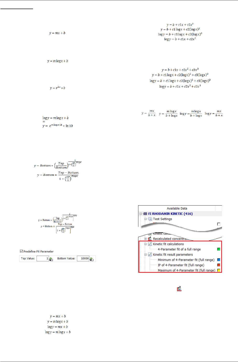
Omega Software Manual - Part III: MARS Data Analysis
BMG LABTECH
27.07.2017
0415F0045A
56/81
Available methods:
Linear regression fit: Calculates a straight line through the
kinetic range with minimum r² value. The result describes the
line with the parameters m (slope) and b (offset):
.
Logarithmic fit: Calculates a logarithmic curve through the
kinetic range with minimum r² value. The result describes the
curve with the parameters m (scale) and b (offset):
Exponential fit: Calculates an exponential curve through the
kinetic range with minimum r² value. The result describes the
curve with the parameters k and b:
Double logarithmic fit: Calculates a logarithmic curve through
the kinetic range with minimum r² value, where the y values are
also logarithmic. The result describes the curve with the
parameters m and b:
4-Parameter fit: Calculates the dose response curve in the
kinetic range with minimum r² value. Result parameters are
Bottom, Top, Slope, IP (point of inflection) for the formulas (the
first one for logarithmic y values, the second one for linear y
values):
5-Parameter fit: Calculates the dose response curve with a
symmetry factor in the kinetic range with minimum r² value.
Result parameters are Bottom, Top, Slope, IP (point of inflection),
Symmetry for the formulas (the first one for logarithmic y values,
the second one for linear y values):
If the 4-Parameter fit or the 5-Parameter fit is selected,
additional controls appear on the window:
Predefine Fit Parameter: Check this control to predefine the Top
and Bottom value of the fit. Enter a value for Top and Bottom.
Segmental regression fit: The segmental regression divides the
kinetic range into two segments and calculates a linear
regression for each segment. The result of the fit is the result of
each linear regression and the intersection point of the two lines.
Each combination of logarithmic and linear x and y values has its
own fit formula:
2nd polynomial fit: Calculates a quadratic polynomial curve
according to the kinetic range. The result parameters are b
(offset), c1 (multiplier 1) and c2 (multiplier 2) for the fit formulas:
3rd polynomial fit: Calculates a third order polynomial curve
according to the kinetic range. The result parameters are b
(offset), c1 (multiplier 1), c2 (multiplier 2) and c3 (multiplier 3)
for the fit formulas:
Hyperbola fit: Calculates a hyperbola in the kinetic range with
minimum r² value. Each combination of logarithmic and linear x
and y values has its own fit formula:
User defined fit: Define you own fit formula, if none of the
predefined formulas fulfill your requirement. If this entry is
selected, a button Edit Formula... appears. Click on this button to
define the formula and the fit parameters. Details are explained
in the chapter 4.26 User defined fit formulas.
Select fit parameters / enter aliases:
In addition to the fit result curve you can create a result node for
each available fit parameter. Check the check box control for the
parameters you want to use as result. If you want to use a
different name for the result parameter, enter the alias name in
the entry field beside the parameter.
After performing the calculation new nodes appear in the
navigation tree. One for the fitted curve and one for each result
parameter you have selected:
4.10 Standard Calculations
The standard calculation page is only enabled if the layout of
the test run contains standards. If the test run is a kinetic
measurement, a kinetic calculation must be performed first to
enable the standard calculation page. If the test run is a
measured spectrum, at least one discrete wavelength must be
added to the test run, to enable the standard calculation page.

BMG LABTECH
Omega Software Manual - Part III: MARS Data Analysis
57/81
0415F0045A
27.07.2017
Input data: Select the input data for the standard calculation.
This can be the result of any calculation generating end point
data. If the selected input data has kinetic data, you need to
select the cycle/interval to define the data base for the fit. If the
layout contains replicates of the standards and the selected is
not based on a replicate calculation, you can define that the
calculation is based on the average of the replicates if you check
the control use average of replicates to calculate the standard
curve.
Calculation method: Select the curve fitting method for the
standard calculation. Each curve fitting calculation has a set of
parameters that describes the fit result and is used for the
concentration recalculation of the samples. See the section Fit
Results below for more information.
Available methods:
Linear regression fit: Calculates a straight line through the
standards with minimum r² value. The result describes the line
with the parameters m (slope) and b (offset):
If force line through zero is selected the linear regression fit
calculates a straight line with Y=0 for X=0:
4-Parameter fit: Calculates the dose response curve for the
standards. Result parameters are Bottom, Top, Slope, EC50/IC50
and log(EC50)/log(IC50) for the formula:
The variable IP (point of inflection) in the Formula is the
EC50/IC50 value. The first formula is used if logarithmic Y values
are used, the second is for linear Y values (see Linear or
logarithmic X / Y Values below)
5-Parameter fit: Calculates the dose response curve with a
symmetry parameter for the standards. Result parameters are
Bottom, Top, Slope, Inflection point, EC50/IC50,
log(EC50)/log(IC50) and Symmetry for the formula:
The variable IP (point of inflection) in the Formula is the
Inflection point value. The EC50/IC50 is the concentration value
where the signal is in the middle between Top and Bottom. The
first formula is used if logarithmic Y values are used, the second
is for linear Y values (see Linear or logarithmic X / Y Values
below)
advanced 5-Parameter fit: Select the 5-Parameter fit method
and click the Use advanced 5 parameter fit to get this calculation
method. It calculates the dose response curve with a symmetry
parameter for the standards, but without moving the point of
inflection. Result parameters are Bottom, Top, Slope, EC50/IC50,
log(EC50)/log(IC50) and Symmetry for the formula:
The variable IP (point of inflection) in the Formula is the
EC50/IC50 value. The first formula is used if logarithmic Y values
are used, the second is for linear Y values (see Linear or
logarithmic X / Y Values below)
If the 4-Parameter fit or the 5-Parameter fit is selected,
additional controls appears on the window:
Use EC/IC: Defines if EC or IC value should be calculated.
Predefine Fit Parameter: Check this control to predefine the Top
and Bottom value of the fit. Enter a value for Top and Bottom.
Cubic spline fit: A spline is a special function defined piecewise
by polynomials. The cubic spline calculates polynomial fit curves
between two adjacent standards. The result is a continuous and
differentiable curve with each standard lying on the curve.
Therefore the result is not just one formula but a set of
polynomial formulas and r² is always 1.
Point to point fit: The point to point fit calculates linear
regression fits between two adjacent standards. The result is in
fact a continuous but not a differentiable curve. Each standard is
lying on the curve therefore the result r² is 1.
Segmental regression fit: The segmental regression divides the
standards into two segments and calculates a linear regression
for each segment. The result of the fit is the result of each linear
regression and the intersection point of the two lines.
2nd polynomial fit: Calculates a quadratic polynomial curve
according to the standards. The result parameters are b (offset),
c1 (multiplier 1) and c2 (multiplier 2) for these fit formulas (one
formula for each combination of linear and logarithmic X and Y
values. See Linear or logarithmic X / Y Values below):

Omega Software Manual - Part III: MARS Data Analysis
BMG LABTECH
27.07.2017
0415F0045A
58/81
3rd polynomial fit: Calculates a third order polynomial curve
according to the standards. The result parameters areb (offset),
c1 (multiplier 1), c2 (multiplier 2) and c3 (multiplier 3) for these
fit formulas (one formula for each combination of linear and
logarithmic X and Y values. See Linear or logarithmic X / Y Values
below):
Hyperbola fit: Calculates a hyperbola for the standards with
minimum r² value. The result parameters are m and b for these
fit formulas (one formula for each combination of linear and
logarithmic X and Y values. See Linear or logarithmic X / Y Values
below):
User defined fit: Define you own fit formula, if none of the
predefined formulas fulfill your requirement. If this entry is
selected, a button Edit Formula... appears. Click on this button to
define the formula and the fit parameters. Details are explained
in the chapter 4.26: User defined fit formulas.
Linear or logarithmic X / Y Values: Use the check boxes available
to define whether the fit result is shown using either linear or a
logarithmic scaling for the according axes.
Depending on the X and Y Values, a logarithmic calculation may
not be possible (i.e. for values <= 0). In this case the hint
Calculation of fit parameters not possible appears where the fit
result parameters are normally shown.
Note: Using logarithmic X values will influence the fit result of
a point to point fit, a linear regression fit and a segmental
regression fit. Using logarithmic Y values will influence the fit
result of all fit methods.
Use dilution factor for standards calculation: This option
appears if there is at least one dilution factor > 1 defined in the
layout. If this checkbox is checked, the dilution factor is used for
the recalculation of the concentration values meaning that the
result will be multiplied by the dilution factor defined
Use result of group ... for calculation: This option appears if you
have more than one group with standards. It is possible to select
that the standard fit result of one group be used for the
recalculation for all other groups. If the '–' entry is selected then
every group will use its own fit result for the recalculation of the
concentration values.
Don't use wells exceeding limitations for recalculated
concentrations (toggle out): If this option is set, a well will be
automatically toggled out, if a concentration value cannot be
calculated with the resulting fit formula and the value of the well
or if the recalculated concentrations exceeds the limitations (see
Limitations for Recalculated Concentrations). Standards used to
calculate the fit will not be toggled out, because this would
change the fit.
Weighted fit
Check this control if the weight of each standard should not be
the same. You can give less weight to less precise standards and
more weight to more precise standard. Select one of the offered
weighting methods to define, how the weighting for each
standard should be calculated.
Confidence Interval Settings
For all fit methods except the point to point and the cubic spline
fits, confidence intervals and confidence band are calculated
automatically. Confidence intervals are calculated for each
standard and for each fit result parameter. The confidence band
can be displayed in the standard curve chart together with the
error bars. The confidence values for the fit result parameters
are displayed as two additional columns in the fit result table.
CI percentage: Define the percentage value for the confidence
interval calculation. A lower value results in a wider interval
band.
Prediction Bounds Settings: Select between the different
settings:
Observation or Function Bounds: Provides a confidence interval
for a new observation or for a new function (curve).In general,
observation intervals are wider than function intervals, because
of the additional uncertainty of predicting a new response value
(the function plus random errors).
Non-simultaneous or Simultaneous Bounds: Provides a
confidence interval using a single predictor value (non-
simultaneous) or all predictor values (simultaneous). In general,
simultaneous intervals are wider than non-simultaneous
intervals, because of the additional uncertainty of bounding
values for all predictors.
4.10.1 Fit Result
After performing a standard curve fit, the fit result can then be
inspected on the standard curve chart. If this is the first standard
calculation of the test run, the tab for the standard curve page
will appear following a successful fit.
If a fit fails for a group of standards of the test run, the hint
Calculation of fit parameters not possible appears on the detailed
window for the fit result and on the fit result window. The
reason for a failed fit could either be a wrong axis scaling
(logarithmic instead of linear), or a less number of standards to
calculate the fit (see Limitations for Recalculated Concentrations)
If the calculation of a concentration value fails for a well, you will
see in the microplate or table view a text message that indicates
the reason for the failure:
In the microplate and the table view, the result of the
concentration calculation for the contents, based on the fit result
will be displayed.
Text
Meaning
n.a.
Not available - recalculation not possible (normally the fit
itself was not possible)
<< std
range
The calculated concentration value is under the defined limit
for this calculation method. (see Limitations for Recalculated
Concentrations table below)
>> std
range
The calculated concentration value is above the defined limit
for this calculation method. (see Limitations for Recalculated
Concentrations table below)
<< Y range
The input value is either under the domain of the fit or under
the defined limit for this calculation method. (see Limitations
for Recalculated Concentrations table below)
>> Y range
The input value is either above the domain of the fit or above
the defined limit for this calculation method. (see Limitations
for Recalculated Concentrations table below)
ambiguous
The input value is ambiguous, that means that it fits to more
than one concentration value.
Limitations for Recalculated Concentrations:
Fit method
input (y)
minimum
input (y)
maximum
concentration
minimum
concentration
maximum
min. no.
of
standards

BMG LABTECH
Omega Software Manual - Part III: MARS Data Analysis
59/81
0415F0045A
27.07.2017
Linear
regression
no limit
no limit
no limit
no limit
1
4-
Parameter
Bottom
Top
minX* x 0.5
maxX* x 1.5
4
5-
Parameter
Bottom
Top
minX* x 0.5
maxX* x 1.5
4
Cubic
spline
min Y of
calculated
splines
max Y of
calculated
splines
minX*
maxX*
4
Point to
point
minY*
maxY*
minX*
maxX*
2
Segmental
regression
no limit
no limit
no limit
no limit
4
2nd
polynomial
no limit
no limit
minX* x 0.5
maxX* x 1.5
3**
3nd
polynomial
no limit
no limit
minX* x 0.5
maxX* x 1.5
4**
Hyperbola
no limit
m
no limit
no limit
3
*) minY = minimum value of standards; maxY = maximum value of
standards; minX = minimum standard concentration; maxX = maximum
standard concentration.
**) if less standards are defined, the degree of the polynomial fit will be
reduced (e.g. from 3nd to 2nd if only 3 standards are available or from
2nd to linear regression if only 1 or 2 standards are available)
4.11 Concentration Calculations
The concentration calculation page allows you to perform
arithmetic operations based on recalculated concentration
values (by a standard curve fit calculation) and known
concentrations (standard concentrations).
With these calculations only values of wells which contain a
standard with a defined standard concentration value are
considered.
Input data: Select the input data for the calculation. This can be
the result of any standards calculation with concentration values
as result data.
Calculation: Select the calculation method for your calculation.
Available methods:
Difference of calculated and known concentration: Subtracts the
calculated concentration value from the standard concentration
value.
Ratio between known and calculated concentration: Calculates
the ratio between the known and the calculated concentration.
The result will be multiplied with the entered ratio multiplier.
Ratio between calculated and known concentration: Calculates
the ratio between the calculated and the known concentration.
The result will be multiplied with the entered ratio multiplier.
Percentage deviation of calculated from known concentration:
Calculates the deviation in percent of the calculated
concentration from the known standard concentration. If the
calculated value is less than the standard concentration, the
percentage value is expressed as negative value.
Ratio Multiplier: Enter a ratio multiplier for the calculation.
4.12 Data Calculations
The data calculation page allows you to perform arithmetic
operations between either two different data inputs or between
two sets of wavelength data for the same data input.
First input data: Select the first input data for the data
calculation. This can be the result of any calculation which
outputs the data as numbers.
Second input data: Select the second data input for the data
calculation. This can be the result of any calculation which
outputs the data as numbers.
Wavelength: If the selected input data has more than one
measured wavelength, it is possible to select the wavelength on
which the calculation should be performed. If you select the
entry All in the list, the calculation will be performed for each
wavelength (wavelength 1 of the first input data with
wavelength 1 of the second input data, wavelength 2 of the first
input data with wavelength 2 of the second input data and so
on). If the selected input data contains spectra data and you
select spectrum, the calculation will be done based on the
spectrum curve and the result is again a spectrum curve.
Kinetic Parameters: If the selected input data contains kinetic
data, the Kinetic Parameters controls are visible and can be used
to define how to handle the kinetic data:
Cycle/Interval: select a certain cycle to use only this value for the
calculation. Select all, to do the calculation for all cycles (the
result is than a kinetic curve).
Range: Select a range and a calculation to calculate a certain
value for the cycles/intervals in the range and use this value for
the data calculation.
Multiplier: Enter a multiplier for the calculation.
Calculation: Select the calculation method for your data
calculation.
Available methods: minus, divided by, plus, multiplied by.
values as percentage: This control appears, if the selected
calculation method is 'divided by'. Select it to calculate the ration
as a percentage value. The Multiplier will then be set to 100 and
the resulting unit is %.
Resulting unit: Select the unit type of the calculation result.
4.13 Validations
The validations page lets you classify your data. Similar to the
color modes for the Microplate View, the data can be grouped
into good or bad (pass or fail) categories:

Omega Software Manual - Part III: MARS Data Analysis
BMG LABTECH
27.07.2017
0415F0045A
60/81
Input data: Select the input data for the validation. This can be
the result of any calculation which outputs the data as numbers.
Mode: select the kind of validation: good / bad, good / bad /
unknown, gradient or delta band.
For each measured wavelength you can enter a threshold (for
the good / bad mode) or a lower and an upper threshold (for the
good / bad / unknown mode) or a start and a stop value (for the
gradient mode) or threshold and a delta band value (for the
delta band mode). Enter a threshold value that divides the good
from the bad data or defines the lower and upper boundary of
your classification. You can also select contents out of the pull
down list that defines the threshold value. Use the %of entry
field to define a percentage of a content value (e.g. 20 % of the
blank value). In the delta band mode, you define a threshold and
a delta value which defines a range around the threshold. You
can also define if the delta range is an absolute value or a
percentage of the threshold value.
Display: Text and background color is defined here that will be
shown with the result of the classification. For the good / bad
and the good / bad / unknown modes, you can define if wells,
exceeding the defined thresholds should not be used further on.
Therefore the drop down list for the displayed text has the entry
<Don't Use Well>.
If <Don't Use Well> is selected, the subjacent color control
changes to a list control that allows you to define if only wells
with special contents should be set to unused.
Another special meaning has the entry <Value>. If this item is
selected, the value of the well for the selected input data is
displayed together with the selected color as background.
If gradient mode is selected, the drop down list contains the
additional entry <Percentage>. If you select this entry, not the
value but a percentage representation of the value based on the
entered start and stop values will be displayed.
<= or < (Lower) Threshold (not for the gradient mode or delta
band mode): Select the text displayed for the values under/equal
to the (lower) threshold out of the drop down list, or enter any
text into the entry field and select a according background color.
: Use this control to decide if the value should be lower or
equal or real lower.
<= or < Upper Threshold (only for the good / bad / unknown
mode): Select the displayed text for the values above the (upper)
threshold out of the drop down list, or enter any text into the
entry field and select an according background color.
: Use this control to decide if the value should be higher or
equal or real higher.
between Lower Threshold and Upper Threshold (only for the
good / bad / unknown mode): Select the displayed text for the
values between the lower and the upper threshold out of the
drop down list, or enter any text into the entry field and select an
according background color.
Start Color / End Color (only for the gradient mode): Select the
background color for the start and for the stop value. All values
between these two values will be displayed with a background
color between the two selected colors according to the
percentage of the position of the value between the start and
the stop value. Select Rainbow colors if the background color
should follow the color of the rainbow spectrum.
Outside Band / Inside Band (only for the delta band mode):
Select the displayed text and background color for values outside
the defined delta value around the threshold and for values
inside the defined band.
4.14 Assay Quality
The assay quality calculations page provides several methods
to analyze your measurement.
Input data: Select the input data for calculating the assay quality.
This can be the raw data or the result of any calculation.
Calculation method: Select the calculation method for your
assay quality.
Available methods:
Z' (Z prime): Calculates the Z prime value based on the reference
contents you define. Select a content out of each drop down list
for each of the data on which the Z prime calculation is based on.
The formula for the calculation is:
µ 1 is the average of the values over the replicates of the first reference
content
is the standard deviation over the replicates of the first reference
content.
µ 2 is the average of the values over the replicates of the second
reference content
is the standard deviation over the replicates of the second reference
content.
Signal to blank: Calculates the Signal to blank ratio for each well.
You can select the content which represents the blank value with
the select blank drop down list. If the layout contains blanks, it
will be preselected. The formula for the calculation is:
µ signal is the average of the values over the replicates of the content for
which the S/B value is calculated.
µ background is the average of the values over the replicates of the
blank.

BMG LABTECH
Omega Software Manual - Part III: MARS Data Analysis
61/81
0415F0045A
27.07.2017
Signal to noise: Calculates the Signal to noise ratio for each well.
You can select the content which represents the noise value with
the select noise drop down list. If the layout contains blank, it will
be pre-selected. The formula for the calculation is:
µ signal is the average of the values over the replicates of the content for
which the S/N value is calculated.
signal is the standard deviation over the replicates of the content for
which the S/N value is calculated.
µ background is the average of the values over the replicates of the noise
(blank).
background is the standard deviation over the replicates of the noise
(blank).
Note: It is important to have enough replicates for a
reasonable Z', Signal To Blank or Signal To Noise
calculation. Make sure that the input data for these
calculation methods are NOT the result of a replicate
statistic or based on a replicate statistic!
Percentage calculation: Set the value of each well in a
percentage relation between a 0% and a 100% reference. You
can select the content which represents the 0% reference value
and the content which represents the 100% value. If the 0%
value or the 100% value should be a fixed number (like 0% = 0),
you can enter the value in the related entry field.
In addition, you can enter a percentage value to use e.g. 90% of
the 100% reference or 110% of the 0% reference. The formula
for the calculation is:
µ 0% is the average of the values over the replicates of the 0% reference.
µ 100% is the average of the values over the replicates of the 100%
reference.
Group Handling: If the layout of the test run contains groups,
you have to decide how groups are handled:
Use selected
content for all
groups
Use the selected content of a group for the calculation
even if the calculated well is in a different group.
Calculate for
each group
Use the selected content of the group of the calculated
well. If the group of the well does not have the selected
content, no calculation is done for that well.
Ignore groups
Ignore the groups and calculate the result as if no
groups where defined.
4.15 User Defined Formula
The user defined formula calculation page allows you to
define and perform arithmetic operations based on an entered
equation. The result of the equation for each well defines the
result data of the created process.
Input data: Select the input data for the data calculation. This can
be the result of any calculation which outputs the data as
numbers. The input data defines the used X value in the formula
for each well and each wavelength (if the input data comes with
more than one wavelength).
Calculate for contents: Select the contents for which the formula
is valid. The formula is applied and calculated for all wells
containing the selected contents. You can select one or more
contents in the drop down menu.
Result name: Enter a name that identifies the formula process.
The name defines the name of the process and node name of
that process in the navigation tree.
4.15.1 Enter a formula
Formula: The field formula shows the entered formula. The color
frame and the text below the field show if the formula is valid. A
syntax check is performed after each entry made into the
formula.
Color
Text
Meaning
green
Formula valid
The formula is valid. The apply button is
enabled and can be pressed if the formula is
completely entered.
orange
Formula
incomplete /
Open bracket
The formula is incomplete. An operator or a
parameter for an operator is missing or a
bracket is not closed. Please complete the
formula.
red
Syntax error
The combination of the entered operators,
variables and constants is not valid. Please
correct the entry to make the formula valid.
Use the operator buttons, the entry fields and the drop down
menus (see description below) to enter the formula. Numbers
and simple operators can also be typed in directly in the formula
field. You can set the cursor in the field with the mouse and you
can delete entries with the backspace and the DEL key on the
keyboard.
Description of the buttons above the formula entry field:
Undo the last step(s).
Sets the cursor one position to the left.
Sets the cursor one position to the right.
Deletes the content (an operator, bracket, variable or
constant value) on the left side of the cursor (if you move
the mouse over the button, the content that will be
deleted is marked with a blue background).
Clears the formula entry field.

Omega Software Manual - Part III: MARS Data Analysis
BMG LABTECH
27.07.2017
0415F0045A
62/81
Adding operators and brackets to the formula (operator
buttons):
To add operators to the formula press the according operator
button. The operator will be inserted at the current cursor
position. If an operator has two parameters (like division) the
operator must be between these two operators, e.g. x / S1 (first
enter the x, using the x (well value) button, then press the
division operator button, and then enter the S1, using the
content drop down menu (how to enter variables and constant
values see below). If the operator has one parameter, the
parameter for most of these operators is behind the operator
only for the x² operator, the parameter comes before the
operator and for brackets the parameter is enclosed between
the brackets. A parameter can be a variable, a constant value or
a formula on its own (enclosed in brackets if needed).
Operator
Button
No.
Parameters
Operator description
2
Multiplication between the two parameters
2
Division: First parameter is the numerator;
second parameter is the denominator.
2
Addition between the two parameters
2
Subtraction between the two parameters
1
Calculates the power of the parameter based on
the Euler's number.
1
Calculates the natural logarithm of the
parameter
1
Calculates the logarithm based on 10 (log
10
(x)) of
the parameter
1
Calculates the absolute value of the parameter
(e.g. -5 becomes 5, but 5 remains 5)
1
Calculates the square of the parameter.
1
Calculates the square root of the parameter.
2
Calculates the power of the two parameters. The
first parameters is the mantissa, the second is
the exponent of the power calculation.
1
Negates the parameter: -5 becomes 5 but 5
becomes -5
1
Encloses the parameter in brackets.
Adding variables and constant values to the formula:
You cannot add constant values or variable names directly into
the formula field with the keyboard. Use the controls described
in this section instead to enter your formula. The value or
variable will be inserted at the current cursor position in the
formula entry field.
Fix value
Use the entry field to enter fix number values. Press the OK
button beside the field to add the value to the formula.
Content
Open the drop down menu and select a content. Press the
OK button to add the content as a variable to the formula.
The value of the content, valid for the selected input data
will be used in the formula. If replicates are available, the
average value over the replicates is used. For each group of
contents (Standards, Samples..), there is a separate entry
with the extension iterate over, indicated with a # after the
content type letter (S#, X#, ...) in the formula. Select this
content, if the index of the content should follow the index
of the content of the well, for that the value is calculated.
Example: If the formula is x-S# and the wells content is X2,
the value of S2 will be used at the position of S# in the
formula (X2-S2 will be calculated for that well).
If the layout contains groups, a further drop down menu
appears on the right side of the content drop down menu.
You can select between certain group, <ignore groups> or <
calculate for each>:
<ignore group>: The average of all the wells with the
selected content over all groups will be calculated and used
in the formula. The variable in the formula is marked with
an i: S1i, or X2i...
<calculate for each>: The average of the wells with the
selected content of the group for the current well will be
calculate and used in the formula (if the result for a well of
group A is calculate, the average of the content for group A
is used, if the result for a well of group B is calculated, the
average of the content for group B is used, and so on). The
variable in the formula has no further mark: S1, X2...
GROUPNAME: The average of the wells with the selected
content of the group GROUPNAME will be used in the
formula, regardless of the group of the currently calculated
well. The variable in the formula is marked with the name of
the group: S1A, X2B...
Well
Open the drop down menu and select a well. Press the OK
button to add the well as a variable to the formula. The
value of the well, valid for the selected input data will be
used in the formula.
Add x (x =
input data)
The variable x will be added to the formula, when you press
this button. X is replaced with the value, valid for the
selected input data of the currently calculated well, when
the formula is applied.
dilution of x
The term dil(x) will be added to the formula, when you
press this button. Dil(x) is replaced with the dilution value of
the currently calculated well. If no dilution values where
defined, a dilution of 1 is used.
concentrati
on of x
The term conc(x) will be added to the formula, when you
press this button. Conc(x) is replaced with the
concentration value of the currently calculated well, if
available/defined. If the well is not a standard with
concentration value, no calculation for this well is done.
value... or
variable or
value...
Press this button to add a value that comes from any other
calculation in this test run or a variable to the formula. Read
the chapter 4.2.1: Define and Use Variables to see, what
variables and values are and how to use them. In the
formula, variables are displayed as V1, V2, V3..., values are
displayed as C1, C2..., W1, W2... if they represent content or
well values. If the value represents a fit result parameter,
the name of the parameter is displayed in the formula. If
you move the mouse over a variable or a value in the
formula, you get a detailed hint with information about the
variable or value.
OD(nm)
Returns the OD value for a given Lambda value in nm if the
value is in the valid range of the measured spectrum (only
for Spectrum measurements).
nm(Y)
Returns the nm value of the given Y value of the spectrum
curve. The nm value is the value of the index which is the
nearest to the given Y value (only for Spectrum
measurements).
λ in nm
If the selected input data is a spectral scan, the current
wavelength value of the iteration over the wavelength will
be used in the formula.
Y(time)
Returns the signal value of a given time value if the time
value is in the valid range of the measured kinetic (only for
kinetic measurements).
time(Y)
Returns the time value of the given Y value of the signal
curve. The time value is the value of the index which is the
nearest to the given Y value (only for kinetic
measurements).
t in s
If the selected input data has kinetic data, the current time
value of the iteration over the time will be used in the
formula.
Resulting unit: Enter the resulting unit of the entered formula.
This can be any entered text or you can select one of the entries
of the drop down menu: Use the entry Same as input data, if the
unit of the formula result is the same as the unit of the input
data. Select none if the formula has no unit or you don't know
the unit.
Note: The selected unit affects the used format to display the
numbers. See chapter 3.24.5: Number Format Settings.
4.15.2 Export and Import a Formula
If a formula is valid it can be exported to a file to save it and use
it for further test runs. To use a previously saved formula you can
import the formula:

BMG LABTECH
Omega Software Manual - Part III: MARS Data Analysis
63/81
0415F0045A
27.07.2017
Import
Formula
Press this button to open a file dialog and to import a saved
formula. Files containing a formula have the extension MWF.
Only files with this extension can be selected and opened.
Export
Formula
If the entered formula is complete and valid, you can press this
button to export the formula to a BMG Labtech formula file
(with the file extension MWF). A file dialog opens. Enter the
name for the file (the extension will be added automatically)
and press Save to save the formula to the file.
4.16 Enzyme Kinetic Calculations
The enzyme kinetic calculation page is only enabled if it is a
kinetic measurement and the layout of the test run contains
standards. Read more about enzyme kinetic and how to set an
experiment and use MARS to evaluate the measurement in
Chapter 4.16.4: How to Perform an Enzyme Kinetic Experiment.
The enzyme kinetic calculation algorithm calculates the reaction
velocity over the concentration first. Based on this it performs a
hyperbola or a linear fit - depending on the selected calculation
method -, to evaluate Vmax and Km.
Input data: Select the input data for the enzyme kinetic
calculation. This can be the result of any calculation that keeps
the kinetic data.
Wavelength: If the selected input data comes with more than
one wavelength (multi chromatic, dual channel or spectrum),
select the wavelength for the calculation.
Calculation method: Select the desired enzyme kinetic equation
to perform the fit of the reaction rate over the concentration.
Available methods:
Michaelis-Menten fit: The saturation process describes a
hyperbola. The Michaelis-Menten fit calculates directly the
desired variables Km and Vmax based on this hyperbola:
where Y is the reaction velocity and X is the concentration.
Lineweaver-Burk: Transforms the plot of the reaction velocity (V)
over concentration ([S]) to 1/V (Y-Axis) over 1/[S] (X-Axis) and
performs a linear regression fit:
where VMax = 1/b and Km = m/b
Eadie-Hofstee: Transforms the plot of the reaction velocity (V)
over concentration ([S]) to V (Y-Axis) over V/[S] (X-Axis) and
performs a linear regression fit:
where VMax = b and Km = -m
Scatchard: Transforms the plot of the reaction velocity (V) over
concentration ([S]) to V/[S] (Y-Axis) over V (X-Axis) and performs
a linear regression fit:
where VMax = -b/m and Km = -1/m
Hanes-Woolf: Transforms the plot of the reaction velocity (V)
over concentration ([S]) to [S]/V (Y-Axis) over [S] (X-Axis) and
performs a linear regression fit:
where VMax = 1/m and Km = b/m
Concentration unit: Enter the concentration unit. If the
concentration unit is already defined, you can see and change it
here.
Kinetic range: Select the range for the calculation of the reaction
velocity (maximum slope in the range). The full range is always
available and covers the total measurement. See in the chapter
4.1 Ranges, how to define a range. All defined ranges are listed
in the drop down list with their start and stop cycle/interval.
Select a range for the calculation from this list. To view, create or
change a range, press the button to open the range
window. You can also define an individual range, where the start
and/or stop cycle/interval is not fix. Select the last entry
(Individual Range) in the drop down list to use and define and
individual range. Read more about individual ranges in the
chapter 4.1 Ranges.
Reaction velocity: Define if the reaction velocity is volume per
microsecond, millisecond, second, minute or hour.
4.16.1 Define Enzyme Dilution Factor(s) and Extinction
Coefficient(s)
Enzyme Dilution Factor: If the enzyme was diluted, enter the
dilution factor in this field.
for Group: (only visible if the layout contains more than one
group) If groups are defined, a dilution factor for each group can
be entered (the control Different dilution factor for each group
must be checked) or the same dilution factor for all groups can
be used. To enter the dilution factor for a certain group, select
the group with the drop down control and enter the desired
factor.
Enter Extinction Coefficient(s): If this control is selected, the
extinction coefficient to transfer the OD values to concentration
volumes must be entered below. Read more about how to find
out the extinction coefficient with MARS in chapter 4.16.4: How
to Perform an Enzyme Kinetic Experiment.
Calculate Extinction Coefficient(s): If this control is selected, the
extinction coefficient to transfer the OD values to concentration
volumes are calculated automatically. Therefore a linear
regression fit is performed on the last cycle/interval of the
selected range, where the slope of the fit defines the coefficient.
This is only possible in long-time enzymatic reactions in which
the substrate is completely converted into product indicated by
no more change in signal. Read more about how to find out the
extinction coefficient with MARS in chapter 4.16.4: How to
Perform an Enzyme Kinetic Experiment.
Extinction Coefficient: If Enter Extinction Coefficient(s) is
selected above, this field is enabled and the extinction coefficient
can be entered in this field.
for Group: (only visible if the layout contains more than one
group) If groups are defined, an extinction coefficient for each
group can be entered (the control Different extinction
coefficient for each group must be checked) or the same

Omega Software Manual - Part III: MARS Data Analysis
BMG LABTECH
27.07.2017
0415F0045A
64/81
extinction coefficient for all groups can be used. To enter the
extinction coefficient for a certain group, select the group with
the drop down control and enter the desired value.
4.16.2 Consider zero concentration reaction
Subtract reaction of content with zero concentration: If you
have a background reaction at concentration zero, that needs to
be subtracted from the reaction with concentration, check this
control and select the content which contains the substance with
concentration zero with the next control:
Select the content with concentration zero: Select the content
from the drop down list that contains the substance that shows
the reaction with no concentration.
Group Handling: If the layout of the test run contains groups,
you have to decide how groups are handled:
Use selected
content for all
groups
Use the selected content of a group for the calculation
even if the calculated well is in a different group.
Calculate for
each group
Use the selected content of the group of the calculated
well. If the group of the well does not have the selected
content, no calculation is done for that well.
Ignore groups
Ignore the groups and calculate the result as if no
groups where defined.
4.16.3 Calculation Result
After performing an enzyme kinetic calculation, the result can
then be inspected on the enzyme kinetic fit chart. If this is the
first enzyme kinetic calculation of the test run, the tab for the
enzyme kinetic fit curve page will appear following a successful
calculation.
The calculated Vmax and Km values are displayed in the detailed
window and can be displayed and exported on the enzyme
kinetic fit result window.
In the microplate and the table view, the calculated reaction
velocity for each well is shown for that calculation node.
4.16.4 How to Perform an Enzyme Kinetic Experiment
This chapter describes how to set an experiment and how to use
the MARS Data Analysis software for the determination of Km
and Vmax.
Outline
1. Definition of Km and Vmax
2. Preparation of the standard curve
3. Enzymatic measurements using different substrate
concentrations
4. Evaluation using the MARS Data Analysis software
Definition of Km and Vmax
Km (Michaelis-Menten constant) is equivalent to the substrate
concentration at which the reaction velocity reaches half of the
maximal velocity. Km describes the affinity of enzymes to a
specific substrate.
Vmax stands for the maximal velocity of an enzymatic reaction.
Preparation of the standard curve
A usual enzymatic reaction contains a substrate that is converted
into a product with the help of an enzyme. To determine the
conversion from substrate to product it is necessary that the
substrate changes its spectral properties during the reaction.
Either the substrate absorbs at a special wavelength and does
not give a signal when it is converted to the product or the
substrate gives no signal but the product does. The following
figure shows a reaction example in which the product gives a
measurable absorbance signal:
The product pNP (p-nitro phenol) is a yellow substance and
shows an absorbance maximum at about 410 nm whereas the
substrate pNPA (p-nitro phenyl acetate) does not show any
absorbance at 410 nm.
Self-made standard curve
Before the enzymatic measurement will start a standard curve of
the substrate/product should be taken. The slope of the
standard curve will later be necessary for the enzymatic kinetic
calculations. An example for the pNP standard curve is given
here:
Software made standard curve
In case that the enzymatic reaction is run until the substrate is
completely converted into the product, it is possible that the
software creates the standard curve using the endpoint values of
the wells. Please note that this option is only useful when the
substrate is completely converted into the product indicated
measurement values that are no longer increasing or decreasing
(plateau). This kind of kinetic measurements usually take several
hours.
Enzymatic measurements using different substrate
concentrations
Usually equal amounts of enzyme solution and buffer are
transferred into the wells. Different concentrations of substrate
are added using the onboard injectors. A possible layout is given
here:
The blank should contain everything except the enzyme. The
negative control should contain everything except the substrate.
Evaluation using the MARS Data Analysis software
After measurement the results can be found in the MARS Data
Analysis software. First it is necessary to take a look at the signal
curve. An example is given here:

BMG LABTECH
Omega Software Manual - Part III: MARS Data Analysis
65/81
0415F0045A
27.07.2017
Choose a range that is useful for the calculation of the maximum
slope. The range should be right shifted from the injection peaks.
After that, open the calculation window and click the tab Enzyme
Kinetic. The following window will appear:
Now you have to choose the input data – that is usually blank
corrected raw data or average based on blank corrected data.
For the calculation method you can choose between the
Michaelis-Menten-Fit, Lineweaver-Burk, Eadie-Hofstee,
Scatchard and Hanes-Woolf.
It is very important to type in the unit of the substrate
concentrations used. In this case it was µmol per minute. Select
the correct range that was defined before in the Signal Curve
window. In case that the enzyme was diluted the dilution factor
should be announced.
The extinction coefficient can either be typed in (the slope of the
standard curve) or can be calculated automatically.
Note: Please note that the automatic calculation of the
extinction coefficient is only possible in long-time
enzymatic reactions in which the substrate is
completely converted into product indicated by no
more change in signal.
Consider zero concentration reaction:
Subtract reaction of content with zero concentration: If you run a
background reaction at a concentration of zero (but that is not
identical to the blank), and you want to subtract this value from
all other values, check this control.
Select the content with concentration zero: Select the content
that contains the substance with zero concentration from the
drop down list (e.g Positive Control).
Group Handling: If the layout of the test run contains groups, you
have to decide how groups are handled:
Use selected content for all groups: Use the selected content of a
group for the calculation even if the calculated well is in a
different group.
Calculate for each group: Use the selected content of the group
of the calculated well. If the group of the well does not have the
selected content, no calculation is done for that well.
Ignore groups: Ignore the groups and calculate the result as if no
groups where defined.
4.17 Curve Scaling
The Curve Scaling calculation converts a signal curve or a
spectrum curve to a percentage presentation between a defined
maximum (100%) value of the curve in the selected range and a
defined minimum (0%) value. This calculation can be used to
normalize the curves:
Input data: Select the input data for the calculation. This can be
the raw data or the result of any calculation that obtains kinetic
data or spectra data.
If the input data has both, kinetic and spectra data, you can
select if the scaling should be calculated based on the kinetic or
based on the spectra curve with the radio control above the
input data drop down list: Scale kinetic curve / Scale Spectrum
curve
Select range: The input data for a curve scaling calculation are
always defined by the first cycle/interval and the last
cycle/interval of a kinetic range or by the first wavelength and
the last wavelength of a spectrum range. It is possible to have
one or more ranges defined. The full range is always available
and covers the total measurement. See the chapter 4.1: Ranges,
how to define a range. All defined ranges are listed in the drop
down list with their start and stop cycle/interval or wavelength
(depending on the selected input data). Select a range for the
calculation from this list. Only ranges with at least three values
are shown, because the minimum number of values for the curve
analysis is three. To view, create or change a range, press the
button to open the range window. You can also define an
individual range, where the start and/or stop value is not fix.
Select the last entry (Individual Range) in the drop down list to
use and define and individual range. Read more about individual
ranges in the chapter 4.1: Ranges.
100% Value: Select if the 100% value comes from the maximum
of the curve in the selected range or if it is a fix value. Fix values
can be entered in the Value entry field. The fix value can also
come from a defined variable (see Variables).
0% Value: Select if the 0% value comes from the minimum of the
curve in the selected range or if it is a fix value. Fix values can be
entered in the Value entry field. The fix value can also come from
a defined variable (see Variables).

Omega Software Manual - Part III: MARS Data Analysis
BMG LABTECH
27.07.2017
0415F0045A
66/81
Example:
4.18 Spectrum Calculations
The spectrum calculation page allows you to define a
calculation based on a range over a measured spectrum. You can
only select it, if the test run is a spectrum scan test.
Input data: Select the input data for the calculation. This can be
any process with spectrum data.
Spectrum range: The input data for a spectrum calculation are
always defined by the first wavelength and the last wavelength
of a range. It is possible to have one or more ranges defined over
your spectrum. The full range is always available and covers the
total measurement. See in the chapter 4.1: Ranges, how to
define a range. All defined ranges are listed in the drop down list
with their start and stop wavelength. Select a range for the
calculation from this list. To view, create or change a range, press
the button to open the range window. You can also
define an individual range, where the start and/or stop
wavelength is not fix. Select the last entry (Individual Range) in
the drop down list to use and define and individual range. Read
more about individual ranges in the chapter 4.1: Ranges.
Calculation method: Select the calculation method for your
spectrum calculation.
Available methods:
Sum: Calculates the sum of all measurement values for all
measured wavelengths within the selected range for each well.
Maximum: Finds the measured maximum value within the
selected range for each well.
Minimum: Finds the measured minimum value within the
selected range for each well.
Local maxima: Calculates all local maxima within the selected
range for each well. See an example of local maxima or minima
in the picture below.
For each maximum found, a node in the workflow tree will be
created to see the associated value(s) of the maximum for each
well (and cycle if it is a kinetic test run). See the section Extended
parameters and created result for Local Maxima, Local Minima
and Inflection points below for more details. In the same section
you can find an explanation of the additional parameters you can
use for this calculation method.
Local minima: Calculates all local minima within the selected
range for each well. See an example of local maxima or minima
in the picture below.
For each minimum found, a node in the workflow tree will be
created to see the associated value(s) of the minimum for each
well (and cycle if it is a kinetic test run). See the section Extended
parameters and created result for Local Maxima, Local Minima
and Inflection points below for more details. In the same section
you can find an explanation of the additional parameters you can
use for this calculation method.
Inflection points: Calculates all inflection points within the
selected range for each well.
For each inflection point found, a node in the workflow tree will
be created to see the associated value(s) of the inflection point
for each well (and cycle if it is a kinetic test run). See the section
Extended Parameters and Created Result for Local Maxima, Local
Minima and Inflection points below for more details. In the same
section you can find an explanation of the additional parameters
you can use for this calculation method.
Average: Calculates the average of all measured values within
the selected range for each well.
Slope: Calculates the linear regression curve for the measured
points in the selected range and gives the corresponding slope
value for each well.
Maximum of slope: Finds the maximum slope value of all
measured points within the selected range for each well. The
slope is calculated using the entered width: A linear regression fit
with the number of measured values entered in the width entry
in the Parameters group is performed, starting with the first
wavelength of the range up to the last. The maximum value of all
calculated slopes is the result. You can decide with the Slope
Direction control in the Parameters group whether the rising or
the falling maximum value should be calculated.
Wavelength at threshold: Calculates the wavelength taken from
the first wavelength in the selected range for the curve to reach
a given threshold for each well. Enter the threshold value in the
entry field Threshold, this option appears under the smooth
controls when this method is selected. If a spectral curve does
not reach the entered threshold, n.a. will be printed as result.
You can define, what you want to see instead of n.a. in the result
table with the Result, if threshold is not reached drop down
menu.
Output: Select the desired output values. The available output
depends on the selected calculation method. Each selected

BMG LABTECH
Omega Software Manual - Part III: MARS Data Analysis
67/81
0415F0045A
27.07.2017
output type will be displayed in a separate node or group of
nodes in the navigation tree.
Available output types:
OD value: This type is available for all calculation methods
except Wavelength at threshold. It shows the associated OD
Value for the given calculation result.
Wavelength (nm): Not available for the calculation methods
Sum, Average and Slope. It shows the associated Wavelength for
the given calculation result.
Slope direction: Only available for the calculation method
Inflection points. The result can have the values -1 for a falling
direction, 0 for no slope and 1 for a rising direction.
In addition you can smooth the curve before the calculation to
reduce the effect of the noise in the measurement. Check the
Smooth curve before calculation control and define the number
of moving intervals to smooth the curve.
4.18.1 Extended parameters
If one of the calculation methods Local Maxima, Local Minima
or Inflection points is selected, in the Parameters group on the
left side of the window appears a sensitivity slider control:
Use the Sensitivity slider to define the sensitivity of the
calculation. Depending on the spectrum used as input data, a
high sensitivity can lead to many (wrong) hits because of the
noise of the curve. On the other hand, a very low sensitivity
could lead to a bad result as well because of missing real minima,
maxima or inflection points.
Consider that the calculation is done for each valid well of the
selected input data. This means, that each well has its own
minima, maxima and inflection points and the number of
calculated results can differ between the wells. The number of
created result nodes in the navigation tree will be the highest
number of calculated results for all wells in all cycles (if more
than one cycle was measured).
Therefore, if you have measured empty or blank wells, they
should be excluded from these calculations. Use blank corrected
data as input data and toggle out wells with high noise and less
information before executing this calculation.
4.18.2 Preview the smoothed curves
If you are not sure, how the position of the slider and the
entered interval number are affecting the result, you can press
the Preview button to open a preview of the result of the
calculation:
Use the sliders on the left and right side to see how the result
changes. The left slider is only available, if the Smooth curve
before calculation control was checked on the calculation
window.
Change the displayed well with the Select Well drop down list to
see the result for different wells and - if a kinetic with more than
two cycles was measured - select the displayed cycle with the
Select Cycle drop down list. If the positions of the sliders are
optimized and the result is good, press OK to assign the settings
to the calculation window.
4.19 Statistic over Wells
You can perform a statistic over wells, after selecting two or
more wells in the Microplate View. Select the menu item Statistic
over selected wells... in the Microplate Views popup menu or in
the corresponding menu item under the calculations menu to
open this window:
Input data: Select the input data for the well statistic. This can be
the result of any calculation which outputs the data as numbers.
Calculation method: Select the calculation method for your well
statistic.
Available methods: Average, Standard deviation, Standard
deviation n, Standard Error, %CV, %CV n, Minimum, Maximum,
Median, Sum, No. of Values.
The available methods are the same as for the replicate and
group statistics. For details on the methods, see the chapter 4.5:
Statistics.
Press the OK - button on the window to perform the calculation.
4.20 Well Scan Statistics
The well scan statistics page is used to calculate statistics over
scan points inside a well of a well scan test run.
Input data: Select the input data for the well scan statistic. This
can be the result of any calculation that obtains well scan data
(usually only raw data).
Calculation method: Select the calculation method for your well
statistic.
Available methods: Average, Standard deviation, Standard
deviation n, %CV, %CV n, Minimum, Maximum, Median, Sum,
No. of scan points.
The available methods are the same as for the replicate and
group statistics. For details on the methods, see the chapter 4.5:
Statistics.

Omega Software Manual - Part III: MARS Data Analysis
BMG LABTECH
27.07.2017
0415F0045A
68/81
Press the OK - button on the window to perform the calculation.
If areas where defined inside at least one of the wells (see
chapter 3.22: Well Scanning Data, section: Well Scan Area
detection) an additional calculation method is available: No. of
areas. This returns the number of areas defined in the well.
Furthermore you can decide if the calculation should be
performed for the scan points of the entire well or only for the
scan points of the defined areas inside a well:
Note: The well scan statistics average is automatically
calculated and displayed, if a well scan test run will be
opened the first time.
4.21 Standard Calculation Wizard
In most cases it is not necessary to perform each calculation step
by step.
Use the standard calculation wizard instead.
The wizard recommends the suitable calculation steps to apply
to your standard calculation process.
Click Wizard in the Data Reduction group on the Home tab of the
Ribbon. You can find the same control also in the Common group
on the Calculations tab. After you've clicked the control, the
wizard opens:
4.21.1 When Can You Use the Wizard?
To use the wizard, the test run must fulfill the following
conditions:
The layout must contain one or more standards
End point test runs may have a maximum of two measured
wavelength
Kinetic test runs may have a maximum of one measured
wavelength (including single wavelength FP-measurements)
and not more than one injection.
4.21.2 How the Wizard Works
The wizard recommends calculations depending on the layout
and measurement of the test run.
Each available calculation with its parameters is displayed in a
separate box on the window.
The user can decide whether he wants to perform the
recommended calculations or not by checking or un-checking the
check box for each calculation.
The sequence of the calculation is shown from top to
bottom and is indicated by the numbers on the left side of
the wizard window. This means that the result of a
calculation can be used as the input data for the next
performed calculation in the sequence.
The parameters of the single calculations are similar to
performing the calculation separately by using the
calculation window.
Possible Calculations in the Wizard
Blank Correction
This option will appear if blanks are defined in the layout. When
the blank correction is recommended by the wizard, it is checked
and always the first calculation step. Uncheck the check box if
you do not want to perform a blank correction before creating
the standard calculation.
Wavelength Calculation
This option will appear only for end point test runs with two
measured wavelengths. If you want to plot a standard curve
based on a calculation performed on the wavelengths such as
the ratio between them, leave the Wavelength Calculation check
box checked and select the arithmetic operation you wish to
perform from the drop down list between the two wavelengths.
The available calculations are: minus, divide by, plus or multiplied
by.
If there is a need to swap the wavelengths, select the wavelength
in one of the wavelength drop down lists. The entry for the other
wavelength is updated automatically.
To multiply the result of a division by a constant value, enter the
value into the entry field Ratio multiplier.
Kinetic Calculation
This group appears only for kinetic test runs. If the test run has
an injection, you see two ranges in the group and the injection
cycle / interval number. Otherwise you see only one range.
If only one range is visible, the borders of the range are from the
first to the last cycle/interval of the measurement.
If there are two ranges, the first range includes the
cycles/intervals before the injection, the second range the
cycles/intervals after the injection (including the injection).
To change the borders of the ranges use the spin buttons beside
the entry fields for the start and stop cycles/intervals or enter
numbers into the entry field.

BMG LABTECH
Omega Software Manual - Part III: MARS Data Analysis
69/81
0415F0045A
27.07.2017
Select the calculation method for the kinetic calculation(s). Read
more about kinetic calculation methods in the chapter 4.8:
Kinetic Calculations.
If there are two ranges, two kinetic calculations will be created,
one for each range using the same calculation method.
A kinetic calculation cannot be unchecked, as it is necessary to
perform a kinetic calculation before you can perform a standard
calculation when you have kinetic test runs.
Range Calculation
This option will only appear if the kinetic test run has more than
one range selected or has one injection. In this case you have
two ranges with two kinetic calculations for the two ranges.
It is possible to perform an arithmetic calculation on the two
kinetic calculations (called range calculation in the wizard as the
ranges are defining the kinetic calculations).
Select the calculation method using the drop down list between
the two ranges.
The available calculations are: minus, divide by, plus or multiplied
by.
It is possible to swap the ranges if needed, select a range in one
of the range drop down lists. The entry for the other range will
be updated automatically.
If you want to multiply the result of a division by a constant
value, enter the value into the entry field Ratio multiplier.
If you do not want to perform a range calculation, uncheck the
check box Range Calculation. In this case the standard
calculation will be performed for both kinetic calculations.
Standard Calculation
The last calculation step is always the standard calculation.
Select the curve fitting method you want to perform using the
method drop down list.
If the layout contains dilution factors for at least one sample, the
user can decide whether they want to use the dilution factor for
the recalculation of the concentration values or not.
Using the two buttons shown for the X values and Y values the
user can decide whether to use a linear or logarithmic scale for
each axis.
Read more about standard curve calculation in the chapter 4.10:
Standard Calculations.
After defining all the parameters of the calculations, press the OK
button to perform the calculations.
When the calculation of the standard curve has been completed,
the page with the standard curve will be displayed in the working
area.
If more flexibility is needed to define your calculation than the
wizard provides, you can perform the required calculations step
by step using the calculations window.
4.22 ORAC Evaluation
The ORAC assay is used to determine the antioxidant capacity of
samples. Often Trolox® (a water-soluble analogue of vitamin E) is
used as a standard by which all other antioxidant compounds are
compared. There are three templates available that can be used
to automatically calculate the Trolox® Equivalents (TE) of the
samples.
The ORAC templates can be used if the following criteria are
fulfilled:
1. All samples that are not a blank or a control have to be
defined as standards using different groups for different
substances: The Layout can look like this:
2. Trolox® or any other reference substance should be defined
as standards in group A
3. The concentration of the Trolox® and of the samples should
be typed in using the same unit, e.g. µM or mg/l depending
on what is known about the sample.
If this layout has not been created before starting the
measurement, the layout can be changed afterwards. This is
necessary for using the templates. Please read more about
changing test run layouts in chapter 6 Change Test Run Layout.
4.22.1 Changing the Layout for ORAC Test Runs
For using the easy ORAC evaluation template, all wells containing
samples should be defined as standards in different groups
setting the reference substance (Trolox®) into group A. The
functions of the Change Test Run Layout window can be used as
in the control software for the instrument.
After changing the layout the concentrations of the standard and
the samples have to be defined using the other sheet of the
window Concentrations/Dilutions/Sample IDs.
The concentration unit of the Trolox® and the samples should be
the same, e.g. µM or mg/l. After changing the layout and the
concentrations the changes have to be applied by pressing OK.
To save the changed layout permanently, you have to save the
test run settings.
After changing the layout one of the ORAC templates can be
applied and the calculations of the template will be performed
automatically.
4.22.2 ORAC Templates
The ORAC templates available are:
ORAC no injection
ORAC 1 injection
ORAC 2 injections
The assay can be performed either without using integrated
pumps or with injection of only the ROS generator (e.g. AAPH – 1
injection) or with injection of the fluorophore (e.g. fluorescein)
and the ROS generator (2 injections).

Omega Software Manual - Part III: MARS Data Analysis
BMG LABTECH
27.07.2017
0415F0045A
70/81
How to use templates is explained in chapter 5: Using Templates.
4.22.3 Optimized Settings for ORAC Measurements
The ORAC templates are created for standard measurement
settings and should be adapted if different measurement
settings are used (please use the appropriate template
depending on the number of injections).
Check in the Signal Curve View if the predefined range is covering
the complete time of the measurement. If this is not the case
spread the range manually (see chapter 4.1: Ranges).
4.22.4 Trolox Equivalents (TE Values)
After applying the suitable ORAC template and confirming the
range, the Trolox® equivalents of the Trolox® standards and all
samples are automatically shown in the Microplate View.
The TE values for the reference substance Trolox® should be
close to 1.00. The unit of the TE values is either per µmol, mg or
ml sample depending on what is known about the sample.
The data node showing the TE result is called Concentration
calculations: Ratio calc/known. Next to that the Raw data,
Averages or Linear regression fit results can be viewed, too (see
chapter 3.3: Microplate View)
4.23 Robust Statistics
Robust statistics provides an alternative approach to standard
statistical methods like average, standard deviation and percent
coefficient of variation (%CV).
These estimators are not unduly affected by outliers in a sample
population. You can also use the Remove Outliers function in
MARS to find and remove outliers based on replicates.
Sometimes outliers cannot be found easy and sometimes mask
each other. Using the robust statistics instead of the standard
statistical methods can help to get a better result in such cases.
If the robust statistics is used, equivalents for the mean
(average), the standard deviation and the percent coefficient are
used:
Median instead of mean/average.
robust standard deviation (rSD) instead of SD or SDn: rSD =
MAD x 1.4826 where MAD (median absolute deviation) is the
median of the absolute Value of Xi- Medianx (i iterates over
all replicates of X).
robust percentage coefficient of variation (%rCV) instead of
%CV or %CVn: %rCV = rSD/Medianx* 100%
To activate the robust statistics for an open test run in MARS,
select the control Use Robust Statistics in the Common group on
the Calculations tab of the ribbon menu.
To activate the robust statistics for all new test runs, select the
control Robust Statistics as Default in the Common group on the
Calculations tab of the ribbon menu.
If robust statistics is used in MARS, all calculations based on
average, SD, SDn, %CV and %CVn are recalculated by using the
robust statistics equivalent. A manually performed average
calculation is not affected by this control, but you can change
this calculation manually into a median calculation.
Affected calculations are such as:
Z'
Signal to noise
Signal to blank
Percentage calculations
all calculations using an average over replicates like the
standard fit calculations.
4.24 Curve Analysis
The curve analysis calculation page provides the two main
operations in calculus: Integration and differentiation.
Input data: Select the input data for calculating the curve
analysis. This can be the raw data or the result of any calculation
that obtains kinetic data or spectra data.
If the input data has both, kinetic and spectra data, you can
select if the analysis should be calculated based on the kinetic or
based on the spectra curve with the radio control above the
input data drop down list: based on kinetic curve / based on
Spectrum curve
Select range: The input data for a curve analysis calculation are
always defined by the first cycle/interval and the last
cycle/interval of a kinetic range or by the first wavelength and
the last wavelength of a spectrum range. It is possible to have
one or more ranges defined. The full range is always available
and covers the total measurement. See the chapter 4.1: Ranges,
how to define a range. All defined ranges are listed in the drop
down list with their start and stop cycle/interval or wavelength
(depending on the selected input data). Select a range for the
calculation from this list. Only ranges with at least three values
are shown, because the minimum number of values for the curve
analysis is three. To view, create or change a range, press the
button to open the range window. You can also define
an individual range, where the start and/or stop cycle/interval is
not fix. Select the last entry (Individual Range) in the drop down
list to use and define and individual range. Read more about
individual ranges in the chapter 4.1: Ranges.
Calculation method: Select the calculation method for your
curve analysis.
Available methods:
Area under curve: Calculates the area under the curve in the
selected range using the integration order one. The result is a
single value for each curve that represents the area.

BMG LABTECH
Omega Software Manual - Part III: MARS Data Analysis
71/81
0415F0045A
27.07.2017
Differentiation: Calculates the differentiation curve. Select the
differentiation order in the entry field below the drop down list.
You also can enter a moving interval for the differentiation. If
you use a moving interval > 1, not only the dy/dx value of two
data points are used to calculate the differentiation in one point,
but also the values before and after the data point (moving
interval = 5 means: two value pairs before and two value pairs
after the current value are used).
Integration: Calculates the integration curve. Select the
integration order in the entry field below the drop down list.
Smooth curve for calculation: To get better results with noisy
input data the curves can be smoothed before and after the
differentiation/integration. Read more about the possible
smooth methods in the chapter 4.7: Curve Smoothing.
4.25 Binding Kinetics Calculations
The binding kinetics calculation page is only enabled if it is a
kinetic measurement and the layout of the test run contains
standards.
Input data: Select the input data for the calculation. This can be
the result of any calculation that keeps the kinetic data.
Kinetic range: The input data for this calculation are always
defined by the first cycle/interval and the last cycle/interval of a
range. It is possible to have one or more ranges defined over
your kinetic. The full range is always available and covers the
total measurement. See in the chapter 4.1: Ranges, how to use
and define a range. All defined ranges are listed in the drop
down list with their start and stop cycle/interval. Select a range
for the calculation from this list. To view, create or change a
range, press the button to open the range window. You
can also define an individual range, where the start and/or stop
cycle/interval is not fix. Select the last entry (Individual Range) in
the drop down list to use and define and individual range. Read
more about individual ranges in the chapter 4.1: Ranges.
Calculation method: The binding kinetic calculation comes with
only one calculation method: Kinetic rate equation. It fits the
parameters ka, kd and Rmax of this formula:
Where x is the signals based on the selected Input data and t is
the kinetic time value.
With the Time delayfield, you can define an offset time for the
start of the reaction. The offset is calculated from the first cycle
of the measurement.
4.25.1 Calculation Result
After performing an binding kinetics calculation, the result can
then be inspected on the binding kinetics fit curve. If this is the
first binding kinetics calculation of the test run, the tab for the
binding kinetics fit curve page will appear following a successful
calculation.
The calculated ka and kd and Rmax values are displayed in the
detailed window and can be displayed and exported on the
binding kinetics fit result window.
In the microplate and the table view, the value of the fitted
signal curve for each standard and for the selected cycle is shown
for that calculation node.
4.26 User defined fit formulas
The standard curve fit calculation and the kinetic curve fit
calculation offers a user definable fit formula. To use this fit
formula, select the last entry (User defined fit) in the fit method
pull down list.
After selecting, the window to define the formula opens:
Enter the formula into the Fit Formula entry field and press enter
to apply the formula. The formula will be checked for validity and
parsed to find the containing parameters. If the formula is valid a
table row is created for each fit parameter in the formula. Define
the start parameter for each fit parameter and - if desired - a
lower and upper limit for the parameter.
A useful start value for the parameters is important for the fit
algorithm to find a satisfying result. The closer the start value is
to the expected fit result for this parameter, the faster is the fit
and the better is the fit result.
To add special operators to the formula, you can click on the
operator or functions displayed in the Available operators and
functions control or you can enter them directly in the formula
edit field.
If you've entered the desired and valid fit formula, click OK to
apply the formula to the calculation.
You can change the formula after you've closed this window, if
you click on the Edit Formula button on the dialog where the
calculation is defined.
4.27 Integration Time Wizard
For data with a measured decay curve (only Alphascreen and TRF
measurements) MARS offers a wizard to optimize the integration
start and integration time parameters for further measurements.
If a test run with a measured decay curve is opened in MARS, an
Integration Time Wizard menu in the Data Reduction group on
the Home tab of the Ribbon appears. After clicking this menu
item, the Integration Time Parameter Calculation Wizard opens:

Omega Software Manual - Part III: MARS Data Analysis
BMG LABTECH
27.07.2017
0415F0045A
72/81
Input data: Select the input data for calculating the integration
time matrix. This can be the raw data or the result of any
calculation.
Wavelength 1 / Wavelength 2: If the test runs has more than
one chromatic, select the two relevant chromatics for the
selected calculation. If two different chromatics are selected, the
ration of these two chromatics is used for the calculation.
content with lowest/highest concentration: Select the content
with the lowest concentration and the content with the highest
concentrations.
Calculation: Select the calculation method for your assay quality.
Available methods:
Assay Window: Calculates the ratio between the value of the
lowest and highest concentrations content.
Z' (Z prime) factor: Only available, if replicates are defined in the
layout. Calculates the Z prime value based on the value of the
lowest and highest concentration contents. The formula for the
calculation is:
µ 1 is the average of the values over the replicates of the highest
concentration content
is the standard deviation over the replicates of the highest
concentration content.
µ 2 is the average of the values over the replicates of the lowest
concentration content
is the standard deviation over the replicates of the lowest
concentration content
R² of linear fit: Only available, if standards are defined in the
layout. Calculates a linear fit based on the standards and uses
the resulting r² value to fill the matrix.
LOD (limit of detection): Only available, if standards and blanks
(more than one) are defined in the layout. Calculates a linear fit
based on the standards to get the slope for the LOD formula:
3*SD(blank) / Slope.
SD(blank) is the standard deviation of the blank.
Define the desired input data and calculation and press the
Update Table button to calculate the integration matrix. After
the matrix is calculated, you can adjust the interval settings for
the integration time and integration start range. To recalculate
the matrix with the changed settings, press Update Table again.
Use the color slider on the right side of the table or the color
settings button to adjust the color settings for the table.
5 Using Templates
Templates in MARS are a powerful tool to transfer settings,
performed calculations and even the result of a standard curve
fit to other test runs.
The templates are based on the settings of a test run as they
contain all the information needed for the transfer.
In combination with test run protocols, you can get a quick result
and report of your performed test without any manual action in
MARS needed (see section Why Assign Templates to Protocols?
below)
Individual buttons can be created for up to six templates, giving
the possibility to change quickly between different views for one
test run.
The software comes with a set of predefined templates matching
to the predefined protocols for the readers control software. It is
possible to use these templates to see how they work.
If you want to use your own templates, you must start by
creating a template.
The next step could either be assigning the template to another
test run or to a protocol (read more about assigning a template
to a protocol in the chapter 5.2: Manage Templates).
If you want to use the template often, you can create a button
for that template in the Predefined Templates group on the
Home tab and on the Templates tab of the Ribbon and give it a
name you like. Details are described in the chapter 5.5: Template
Buttons.
If you have a test run with standards and you want to use these
standards to calculate the concentration values of samples in a
different test run, you can do this using a template. Read how
this works in the chapter 5.6: Transfer of Standard Fit Results.
You will soon have a large number of templates. To keep track of
your templates, delete or exchange them for others (export /
import templates), use the manage templates window.
To parametrize the template, you can use variables. You can
decide if the value for the variable will be asked, each time the
template is used, or if a manually entered default value is used.
Read more about variables in chapter 4.2.1: Define and Use
Variables.
Note: Templates are not the tool to transfer modified layouts
from one test run to one other. Use the Manage Layout
functions to exchange layouts between test runs.
5.1 Why Assign Templates to Protocols?
In many cases the templates will be used more than once and
are often applied to test runs, based on the same test run
protocol defined with the BMG LABTECH control software for the
reader.
If you do not want to assign a new template to each new test
run, and equally do not want to add the calculations manually
each time you can overcome this by assigning a template to a
test protocol.
Assign the template to the test run protocol and for these test
runs the template will automatically be assigned to any new
performed test run based on that protocol. When the new test
run is opened for the first time in MARS the settings defined in
the template will be activated.
It is also possible to assign more than one protocol to a template.

BMG LABTECH
Omega Software Manual - Part III: MARS Data Analysis
73/81
0415F0045A
27.07.2017
To manage the templates and the assigned protocols use the
Manage Templates window.
5.2 Manage Templates
To see the existing templates, open the Manage Templates
window. This can be done by clicking Templates in the Manage
Templates group on the Templates tab of the Ribbon.
The window will open and will show the following functions:
A list of all defined templates.
A description of a selected template
Assigned protocols to the template
Function to assign and remove protocols from the template
Function to export and Import templates
Function to delete a template.
5.2.1 List of Templates
The window shows a table with all available templates listed.
The table contains four columns:
Table name: Shows the name of the template.
Allowed methods: The first matching condition: Shows the
measurement methods that match the template. The column
with the allowed methods can contain a small icon with three
dots. This icon appears if the list of matching methods is longer
than the column. Click on the icon to see all matching methods:
Type: The second matching condition: Shows if it is an end point
or a kinetic test run template.
Assigned Protocols: Shows the names of the protocols, assigned
to the template. This column can also contain the icon with the
three dots. Click on it to open a list showing all assigned
protocols.
A template can be selected from the list.
The template description contains a description of the
performed calculations and the settings that will be set if the
template is assigned to a test run.
5.2.2 Change Template Name
To change the name of an existing template, select the template
and click on Change Name.... A small window opens to enter the
new template name.
5.2.3 Assign Protocols to Templates
After selecting a template, press the Assign To Protocol(s)
button, to open a window with a list of the protocols and assign
one or more protocols to that test run.
At the top of the window you will see the name of the selected
template.
The window shows a table with all available protocols in it. The
table consists of four columns:
Protocol name: Shows the name of the test run protocol and
how it was defined in the control software.
Methods: Shows the measurement method for that protocol.
Type: Shows if it is an end point or a kinetic test run protocol.
Template: Shows the name of an assigned template.
LVis: Shows if the protocol uses a BMG LVis Micro Drop plate or
not. This column is only visible, if protocols for the BMG LVis
Micro Drop plate are available.
It is possible to select one or more protocol in the list.
After selecting a protocol, you can immediately check if the
template can be assigned to that protocol using the Verify
Attributes table:
This table shows the two matching conditions for the last
protocol in the list of selected protocols that must be fulfilled to
assign the selected template to that protocol.
The last column of the table shows whether or not the conditions
match (yes, allowed or no; allowed with an orange background,
no with a red background).
If both criteria are fulfilled for all selected protocols, the Assign
button is enabled and can be pressed to assign the template to
the protocols.
If one of the selected protocols has already been assigned to a
template, the link to the old template will be replaced with the
new template.
Enter a protocol name or pattern
Beside the possibility of selecting a protocol from the list of all
available protocols, you can assign a protocol name manually
(e.g. if the protocol will be created later), or you can assign a
pattern with wild cards. If the protocol name matches the
pattern, the template will be assigned to the test run, based on
that protocol. Possible wild cards are * (replaces any number of
signs) and ? (replaces one sign). This gives you the possibility to
assign a template to all test runs created with different
protocols, containing the same pattern in their name.

Omega Software Manual - Part III: MARS Data Analysis
BMG LABTECH
27.07.2017
0415F0045A
74/81
Note: When you assign a protocol name or pattern to the
template, MARS cannot check directly, if the protocol
and the template will fit together. When the test run
will be opened, MARS tries to assign the template if
possible. If not, nothing will be assigned.
5.2.4 Removing Assigned Protocols From the Template
Select a template in the list of templates using the
ManageTemplates window. If there is at least one protocol in
the assigned protocols column, the Remove Protocol(s) button
can be used to eliminate the template link from the protocols.
5.2.5 Edit Parameters
If the selected template contains user defined variables, the Edit
Parameters button is enabled. Clicking the button opens a dialog,
where the variable in the template can be change (default
values, minimum or maximum values...). An explanation of all
different kind of variables and how to use them in calculations
and templates can be found in chapter 4.2.1: Define and Use
Variables.
5.2.6 Export and Import Templates
To export templates, select the templates you want to export
from the list of templates in the Manage Templates window and
press Export....
A file window will open to let you select a file destination for the
saved file containing the exported templates (the look and feel of
the file window depends on the operating system! The shown
window is the file window of Windows Vista.).
Enter a file name for the file and press Save. The generated file
gets the extension .mtf. Files with this extension are recognized
by MARS as exported templates.
To import templates, they must be exported by MARS (e.g. on
another PC) and the file must have the extension .mtf.
Press the Import... button to open a file window similar to the
one above. Select the location of the exported file and select the
file. Press the Open button in the window to import the
template(s) into the list.
5.2.7 Delete Templates
Select one or more templates from the list of templates shown in
the manage templates window. To delete the selected
templates, press the Delete button.
5.3 Create a Template
A new template can be created from the settings used in an open
test run.
This template can then be assigned for use with other test runs
that fulfill the two matching conditions:
The measurement method must be the same
The read type must be the same. An endpoint template
cannot be assigned to kinetic test run and vice versa.
To create a template for use with future test runs you must
perform the test once and open it in MARS to create the
template.
When creating a template, perform the following initial steps:
Open the software and select a test run. The test run should
be the same type as the test run/s you will assign the
template to.
Perform all the data analysis steps with the test run. When
created, the template will then contain all the calculations,
selections, view settings etc. of this test run
Click Create Template from Current Test Run... in the Use
Templates group on the Templates tab or select the menu
item Create Template from the popup menu in the
navigation tree.
On completing the above steps the Create Template window will
then open.
Create template window:
Template name
Enter the name of the template you want to create. The name
must be unique as it will be used to find the template again. If
you want to overwrite an existing template, you can select the
template out of the drop down list. To open the list, press the
drop down button:
Template description
This section describes the steps performed with the test run and
what will be saved in the template. It is possible to expand the
entries with your own explanation of the template. The
description of the template will be displayed to allow the user to
check the suitability of a template before assigning it to other
test runs.
Create CSV/Text file / Create PDF report
If needed, a text (CSV) file and/or a PDF report file can be
created based on the settings in the template, when the
template is assigned to a test run. The settings for the file export
or the PDF report can be defined by pressing the according
Filename and path settings... button.
Assign Template to Test Protocol
A check box is shown at the bottom of the window along with
the name of the test run protocol used to create the template. If
you want to assign the new template directly to that protocol,
leave the check box checked. If you don't want to assign the
template to that protocol, uncheck the check box.
If you want to assign the template to another protocol, you can
do this using the Manage Template window, after creating the
template.

BMG LABTECH
Omega Software Manual - Part III: MARS Data Analysis
75/81
0415F0045A
27.07.2017
Press Create to generate the template. If you want to stop the
creation of the template, press Close.
5.4 Assigning Templates
You can assign a template to a test run or to a protocol (see also
chapter 5.1: Why Assigning Templates to Protocols?).
There are different ways to assign a template to different test
runs or protocols:
5.4.1 Assign a Template to a Test Run
When assigning a template to a test run, the template will be
used to create the settings for the test run. Templates can be
applied to test runs manually if the test run is opened in MARS.
The setting for that test run will also be saved automatically after
successfully assigning a template to the run. The settings of the
test run can still be changed after assigning a template. This is
useful when using templates that perform only the first steps of
your evaluation.
If a test run is signed (FDA 21 CFR part 11), you cannot assign a
template to that test run.
There are four ways in which a template can be assigned to a test
run:
When the test run is opened the first time in MARS and a
template is assigned to the protocol of the test run.
When you select the template, using the Templates control
in the Predefined Templates group on the Home or the
Templates tab (see Chapter 5.5: Template Buttons).
When you have created a template button for that template
and click on the button (see chapter 5.5: Template Buttons).
When you click Assign Template to Current Test Run...in the
Use Templates group on the Templates tab or the menu item
Assign Template of the pop up menu in the navigation tree
and choose the template in the appearing assign template
window.
Assign Template Window
On the top of the window the name of the current test run to
which the template will be assigned is displayed.
Template list and template description
Click on a template in the table to view the description of the
template in the template description area under the table.
The table has three columns:
Table name: Shows the name of the template.
Allowed methods: The first of the two matching conditions:
Shows the measurement methods that match the template. This
column shows the allowed methods and can contain a small icon
with three dots. This icon appears if the list of matching methods
is longer than the column. Click on the icon to see all matching
methods:
Type: The second matching condition: Shows if it is an end point
or a kinetic test run template.
The template description shows the steps the template will
perform on the test run if you assign it.
Verify Attributes
This table shows the two matching conditions for the test run
and the selected template that must be fulfilled to assign the
template to that test run.
The last column of the table shows if the test run conditions
match to the template:
yes: the combination is possible
allowed (with an orange background color): the combination is
possible but with restrictions.
no (with a red background): the combination is not allowed..
If both criteria are fulfilled or at least allowed, the Assign button
is enabled and can be pressed to assign the template to the test
run.
Note: If the template contains kinetic settings but the test
run don't have kinetic data, the combination is allowed,
but the kinetic settings will not be applied to the test
run.
Assign template to test protocol
A check box is shown at the bottom of the window along with
the name of the test run protocol used to create the template. If
you want to assign the new template directly to that protocol,
leave the check box checked. If you don't want to assign the
template to that protocol, uncheck the check box.
Templates with variables
A template can contain variables. You can see if a template
contains variables in the template description. Containing
variables are shown with their variable name (like V1, V2...) and
a description.
The variables in the template will be replaced by certain values if
you assign the template to the test run. Depending on the kind of
variable, the value will be asked to be entered or the defined
default value is used.
Read more about variables in chapter 4.2.1: Define and Use
Variables.
5.4.2 Assign a Template to a Protocol
There are three ways to assign a template to a protocol:
When creating a template (see chapter 5.3: Create a
Template).
When assigning a template to a test run using the assign
window (see Assign Template Window above).
In the Manage Template window.

Omega Software Manual - Part III: MARS Data Analysis
BMG LABTECH
27.07.2017
0415F0045A
76/81
Read more about templates with protocols in the chapter 5:
Using Templates.
5.5 Template Buttons
The Predefined Templates group on the Home tab and on the
Templates tab comes with two default buttons for templates:
. This button gives quick access to all available templates
for the current test run. See the section Templates Button below.
This button creates a new template button in the
Predefined Templates group. The template buttons created
provide quick and easy access to the templates most frequently
used. See the section Add a User Template Button below.
5.5.1 Templates Button
The Templates control in the Predefined Templates group on the
Home tab and on the Templates tab shows a list of all templates
available for use with the current test run. To open the list click
on the button or on the small down arrow on the right side of
the button:
Click on a template in the list to assign that template to the
current test run.
If no template is available for the current test run or if the
current test run is signed the button is disabled.
5.5.2 Add a User Template Button
You can have up to six user template buttons in the Predefined
Templates group. Each button has the same icon in a different
color and an explaining text under the button:
The user button is enabled if the underlying template is
assignable to the current test run. Otherwise the button is
disabled. Pressing the button will assign the template to the
current test run.
If there are less than six template-buttons (if you start the
software first and you have never added a user button before,
there will be no template buttons visible), a new button can be
created by clicking Add Button in the Predefined Templates
group:
New Template Button Window
At the top of the window a table is shown with all available
templates. The table consists of three columns:
Table name: Shows the name of the template.
Allowed methods: The first of the two matching conditions:
Shows the measurement methods that match the template. This
column shows the allowed methods and can contain a small icon
with three dots. This icon appears if the list of matching methods
is longer than the column. Click on the icon to see all matching
methods:
Type: The second matching condition: Shows if it is an end point
or a kinetic test run template.
The template description shows the steps, the template will
perform on the test run if you assign it.
At the bottom of the window you can enter a name for the
button in the entry field Button Name. The entered name will
appear under the button in the Predefined Templates group.
Select the template to be linked to the button in the table.
Click the Create button to add this button representing the
selected template to the Predefined Templates group.
The new button will appear between the last user button created
and the Add Button in the Predefined Templates group.
5.5.3 Changing and Deleting User Template Buttons
Templates associated with a user template button can be
changed and user template buttons can be deleted.
Press the small down arrow on the right side of the button to see
the two menu items with the mentioned functions.
Select Delete Template Button to delete the button.
Select Change Assigned Template... to open the window for
changing the user button:

BMG LABTECH
Omega Software Manual - Part III: MARS Data Analysis
77/81
0415F0045A
27.07.2017
The window is the same as if a new template button is created
(see New Template Button Window above). Additionally it shows
the name of the assigned template at the top of the window. The
assigned template is also selected in the template table.
The associated template and the name of the user template
button can be changed.
Press Assign to accept the changes.
Note: If the user template button is disabled, changing or
deleting the button as described in this chapter is not
available. Use the Manage Template Button window
instead.
5.5.4 Manage Template Buttons
You also can add, change and delete user template buttons with
the Manage Template Buttons window:
Use this window to change or delete a template button if it is
disabled.
5.6 Transfer of Standard Fit Results
If a test run is created without standards in the layout, it is
possible to apply the standard curve fit of another test run to
these samples to calculate the sample concentrations in the
sample test run. Both the sample test run and the standards test
run must be the same type to enable the transfer of the standard
fit from the standards test run to the sample test runs:
Run the measurement for the test run with the standards.
Save the measurement values and open the test run in
MARS.
Perform one or more standard curve fits until you have the
desired fit result.
Delete all performed fits you do not want to have for your
samples.
Create a template from that test run (see chapter 5.3: Create
a Template)
Assign the template to the protocol for the test runs without
standards if you want to have an automatic calculation of the
samples.
Run the measurement(s) for the test run(s) without the
standards.
Open the measured test run with MARS.
If the template was assigned to the protocol, the calculation will
start automatically when the test run is opened. Otherwise the
template with the standard calculation can be assigned after the
test run has been opened.
Blanks will also be transferred to the test run, if the test run with
the standards had blanks and in the layout of the test run are no
blanks defined.
The calculation of the concentration values for each well used in
the test run will then be done and the result can be viewed in the
microplate or table view.
If the template contains more than one standard calculation,
each of the calculations will be performed.
The standard curve of the fit used can also be inspected in the
standard curve chart. The standards in the chart are shown in
gray to indicate that they are not part of this test run.
The transferred standard calculation parameter cannot be
changed anymore and single standards cannot be set to unused.
The regimentation for transferring standard calculations to test
runs with no standards are very small. Only the two conditions to
assign a template to a test run must be fulfilled:
The measurement method must fit
Both test runs must be either end point or kinetic test runs.
Note: To get a valid result you must ensure, that the
measurement conditions are comparable. All
parameters that have a direct influence to the
measurement signal must be identical. See the table
with parameters you have to check below.
Parameter
Measurement
Method
used gain
all
used filter / top or bottom optic
/ used optic type / used optic module / used
wavelength (absorbance spectrum)
all
used microplate (No. wells, plate type, plate color)
all
used volumes
all
No. of used flashes
TRF / HTRF
integration start time and integration time
TRF / HTRF,
Alphascreen
excitation time
Alphascreen
measurement time
Luminescence
temperature
all
focal height (if adjustable - depends on the reader)
all
path length correction
Absorbance
Note: If you use a template with a standard calculation for a
test run that contains standards, the standard
calculation is performed based on the standards in that
test run.
6 Test Run Layout
6.1 Changing Layout
The layout of a measured test run can be changed subsequently
with MARS. You can change each parameter of the layout for the
measured wells in the microplate: The layout content, the layout
group, concentration / dilution values, sample IDs and the
concentration unit. You also can change the plate IDs (1-3) of the
test run.

Omega Software Manual - Part III: MARS Data Analysis
BMG LABTECH
27.07.2017
0415F0045A
78/81
Note: Changing the layout of a test run may affect already
calculated results or even delete a result that cannot
be calculated any more.
The original layout of the test run (the layout of the measured
protocol) is kept and the changed layout can be reset to the
original layout at any time. Deleted results will not be restored
after resetting the layout!
To change the layout of a loaded test run, click Change Test run
Layout in the Test Run Layout group on the Layout tab or press
the button in the layout view window. You also can
click on the change layout icon on top of the Microplate View.
A window with the actual layout opens:
How to change the single parameters of the layout is described
in the next sections of this chapter.
After finishing the changing of the layout, press the OK button to
apply the changes to the test run. A hint window will be
displayed that describes the consequences for the actual
performed calculations. Confirm this dialog to apply the changes.
After applying the changes, the settings of the test run with the
changed layout will be saved automatically. With the
button you can open a stored layout to use it for this test run.
Only saved layouts that match to the test run are provided. The
condition when a layout matches to a test run is described in
Manage Layouts.
To save the layout of the test run and use it with other test runs,
press the button.
Read more about saved layouts in Manage Layouts.
Press the button to undo the last changes.
6.1.1 Changing Plate IDs
To change the plate IDs of the test run, enter the new values into
the Plate ID fields ID 1, ID 2 and ID 3.
Note: The plate IDs of a test run are used to identify a test
run. Consider not to overwrite auto generated IDs if
theses IDs are used as a unique identification of the
test run!
6.1.2 Changing Layout Contents
Changing the contents of a well works the same way as defining
well contents for protocols in the control software. Select the
content type first by clicking the appropriate content button
(Sample, Blank, Standard...) and then use ways to select wells as
described below.
The first letter in the cell of a well indicates the content type
(when fewer than 384 wells are displayed. Otherwise only the
color of the label indicates the content):
X
Sample
The well's content has unknown concentration.
B
Blank
The well contains water or buffer for measuring
background.
S
Standard
The well's content has a known concentration and can be
used to formulate a standard curve.
N
P
C
Negative
Control,
Positive
Control,
Control
The well's content has known concentrations, but will not
be used for the standard curve calculation. It can be used
for comparisons or for special calculations.
The Index is the reference number of the sample or the
standard. The index box displays the number that will be used for
the next well. If increase is selected, each well will be labeled
successively. Constant will keep the same number in the case of
continuous replicates.
If fewer than 384 wells are displayed, the index is the number
behind the content letter. Otherwise only the index is displayed
in the cell.
Replicates are the number of repeated samples or standards in a
row. If you have duplicates on the microplate, you can select the
number of replicates and whether they are labeled in the
horizontal or vertical direction on the microplate.
If you want to use layout Groups (in MARS you can use up to 125
layout groups unlike in the control software where the limit is 26
layout groups), activate the usage of groups with checking the
On check box and select the desired group in the drop down list.
The group will be shown in the layout grid using different
background colors and by inserting the group letter at the end of
the label for the well (if fewer than 384 wells are displayed.
Otherwise only the background gets the according color of the
group). In general, groups are represented by a group letter,
starting with A for the first group and ending with DU for group
number 125. To individualize the representation of the groups,
you can enter Group IDs for each group. Press the
button to open the window, where the group IDs can be entered
and changed:
Methods of selecting wells to fill out the labels:
There are several ways to label the plate, after content, index
and replicate settings are defined:
1. Double click on each well of that type.
2. If the wells of that content are in successive rows or
columns, click on the first well with the left mouse key and
drag across the wells containing the same content.
3. If a total row or column contains the same content, click the
row letter or the column number and all wells of that row /
column will be labeled.
4. To fill the entire microplate click on the format number (e.g.
'96') in the top left corner.

BMG LABTECH
Omega Software Manual - Part III: MARS Data Analysis
79/81
0415F0045A
27.07.2017
Note: Unmeasured wells are disabled in the grid as you
cannot define content for unmeasured wells!
6.1.3 Changing Concentrations, Dilutions and Sample IDs
To change the known concentrations of standards or controls
and the used concentration unit, the dilution factor of samples or
controls or the sample IDs of the contents, go to the
Concentrations / Dilutions / Sample IDs sheet.
The sheet contains a table with all wells of the layout. You can
enter the new concentration or dilution values and the sample
ID.
For the concentrations and dilution values you can use the auto
fill out function that works the same way as entering these
values in the test definition of protocols in the control software.
The table can be sorted, grouped and filtered by the columns
Well Row, Well Col, Content and Group (the group column
appears only if layout groups are used). More information is
given about sorting, grouping and filtering in tables in the
chapter 2.2: Group and Filter Test Runs, as it works the same way
as for test runs.
Concentration values can only be entered for wells with content
type standard, control, positive control and negative control. The
dilution values can only be entered for all wells but not for blanks
and standards.
The auto fill out function can be used to define the
concentrations and dilutions without entering them manually.
The values will automatically be calculated using the given Start
value and a number multiplied with (Factor), added to
(Increment) or subtracted by (Decrement) the last calculated
value.
Click with the left mouse button on the header of the according
column to fill out all wells. You can also select a specific set of
successive wells by selecting them with the left mouse button
down.
Enter the unit for the concentration values in Concentration
unit.
If you enter concentration values, dilution values or sample IDs
and the layout contains replicates, the entered values or IDs will
be assigned to all replicates automatically. To enter different
dilution values or sample IDs for each replicated well the options
Allow different dilution factors for replicates and Allow different
sample IDs for replicates must be activated. To activate these
options, open the MARS Settings dialog (chapter 3.24.1) and
check the appropriate check box controls.
You can use the windows copy and paste function to exchange
data (concentrations, dilutions and/or sample ids) between
MARS and other programs like Excel. To copy data in the list,
select them with the mouse and press the keys Ctrl+C or open
the popup menu with the right mouse button and select Copy. To
import data in the windows clipboard, select the first cell in the
table, where the import should start and press the keys Ctrl+V or
open the popup menu with the right mouse button and select
Paste.
6.1.4 Changing Path Length Correction Settings
If the measurement method of the test run is absorbance or
absorbance spectrum, you can change the settings for the path
length correction. To see and change the settings go to the Path
Length Correction sheet.
Note: This sheet is only available for test runs created with
the reader families OMEGA, PHERAstar version 2.10
and higher, SPECTROstar Nano version 2.00 and higher
or CLARIOstar version 5.00 and higher.
To activate the path length correction, check the according check
box control. Enter the used volume in the wells in the entry field
Volume. The resulting path length is shown in mm. The
absorbance values will be recalculated as values measured with a
path length of 10mm.
To go back to the values defined when the test run was
created/measured, click the Use protocol settings button.
Note: Test runs measured with the BMG LVis Micro Drop
plate do not have a volume field to enter. The path
length of the BMG LVis Micro Drop is known and
independent of the used volume. For these test runs
you only need to switch the correction on or off.
6.1.5 Changing Crosstalk Correction Settings
If the measurement method of the test run is luminescence or
AlphaScreen, you can change the settings for the crosstalk
correction. To see and change the settings go to the Crosstalk
Correction sheet.
Note: This sheet is only available for test runs created with
the reader families PHERAstar or CLARIOstar.
To activate the crosstalk correction, check the according check
box control. Enter the used glow correction factor for
luminescence measurements. For AlphaScreen test runs you
need to define the afterglow correction factor and the glow
correction factor. For dual channel or multichromatic test runs, a
factor for each channel and chromatic must be defined. The
correction can lead to negative values. To prevent negative
values, check the 'Set negative values to zero' control. The raw
data values will be recalculated using the entered correction
factor.
To go back to the values defined when the test run was
created/measured, click the Use determined factor button.
6.2 Manage Layouts
The Manage Layouts function provides you the possibility to
create new layouts or layouts out of a test run, to change the
layouts and to exchange the layouts using the export and import
functionality. These layouts can be assigned to a test run, if the
saved layout fits to the test run.

Omega Software Manual - Part III: MARS Data Analysis
BMG LABTECH
27.07.2017
0415F0045A
80/81
Click Layouts in the Manage group on the Layout tab to open the
manage layout window:
The window contains a list with all saved layouts, containing the
name of the layout and the size of the microplate. The dialog
above shows the layout of a 96 well microplate. After selecting
one layout in the list, the grid on the right side of the list shows
the used wells in the save layout. The plate size and the used
wells are important information as the decision if a saved layout
can be assigned to a test run is based on this information.
6.2.1 Assign a Saved Layout to a Test Run
You can assign saved layouts to test runs. Therefore the two
conditions must be fulfilled:
1. The size of the microplate of the test run and the saved
layout must be identical.
2. The used wells in the saved layouts must be measured wells
in the test run (there can be more measured wells in the
test run but not in the saved layout).
There are four ways to assign a saved layout to a test run:
1. With the manage test run dialog above: Open the test run
and then the manage layouts window. Select one layout in
the list. If the layout can be assigned to the test run, the
Assign to test run button is enabled and must be pressed to
assign the layout..
2. With the menu item Assign Layout to Test Run: Open the
test run and select the menu item. A window similar to the
Manage Layout window shown above, appears.
The list with the saved layouts contains only the assignable
layouts. Select a layout and press OK to assign the layout to the
test run.
3. With the change test run layout window: Press the
button on the window. You see the same window
as shown above. Select the desired layout and press OK. The
layout will be displayed in the Change Layout window and
overwrite the layout displayed before. Press OK on the
Change Layout dialog to apply the new layout.
4. With the Manage Test Run window: Select one or more test
runs of the same microplate size and open the popup menu
by clicking the right mouse button. Select the menu item
Assign Layout. Select the layout and press OK. The layout
will be assigned to each selected test run if possible (see
conditions above). If the layout cannot be assigned to one
or more test runs, a message with a list containing the not
assignable test runs appears.
If a test run is opened, you get a hint how the changed layout will
affect your calculated results.
Note: Plate IDs are not part of the saved layouts and will not
be changed after assigning a saved layout to a test run.
6.2.2 Create and Edit Saved Layouts
Press the New Layout button to create a new layout. After
selecting the size of the microplate the new layout can be
entered as described in. Press the Save button to save the new
layout. You will be asked to enter a name for the new layout.
To view and change a saved layout, select the layout and press
the Edit Layout button. Change the layout as described in
chapter 6.1: Changing Layout and press Save to apply the
changes.
6.2.3 Delete Layouts
Select one or more layouts in the list and press the Delete
Layout(s) to delete the saved layouts.
6.2.4 Export and Import Layouts
You can export the saved layouts and exchange them with
others. Select the layouts you want to export and press the
Export Layouts(s) button. Select a directory to save the layouts.
You can change the recommended filename. The file extension
of the exported layout files is MLF.
To import layouts in a MLF file, press the Import Layout(s) button
and select the directory with the MLF file. Select the file and
press the Import button.
7 Sign a Test Run
To ensure that your measured result and your performed
evaluation on the test run cannot be changed or manipulated
you can sign the test run.
The ability to sign a test run is also needed to fulfill the FDA 21
part 11 compliance. Read more about this in the software
manual part IV: FDA 21 CFR part 11.
To sign a test run, you need a pair of RSA keys. How to get such
keys is also described in the software manual part IV: FDA 21 CFR
part 11.
Click in the Test Runs group on the Home tab of the ribbon
to sign the opened and selected test run. The authentication
window will then appear:

BMG LABTECH
Omega Software Manual - Part III: MARS Data Analysis
81/81
0415F0045A
27.07.2017
After logging in, it is possible to enter a comment to the
signature:
Press OK to finish the sign process.
Signed test runs are indicated with a blue sign text in the test run
description area on top of the working area.
An entry in the audit trail is generated and you can see the
signature on the 21 CFR part 11 pages.
It is possible to add more than one signature to a test run (e.g.
one for released and one for reviewed...)
If a test run is signed, you cannot save any more changes made in
the software for that test run. You can make a copy of the test
run and change the copied test run because the signature will
not be copied.
8 Support
If you have any problem / question regarding the software / the
instruments, you should visit the support section on our web
page (http://www.bmglabtech.com) or contact BMG LABTECH
using the following email addresses:
Problems / questions regarding software:
Problems / questions regarding the instruments:
You can also use our technical request form
(http://www.bmglabtech.com/support/countryselect.cfm).
Note: When you need support from BMG due to a software /
firmware malfunction, you should send us the run log
file together with the error description.
