
Varian APIs
A handbook for programming in the Varian oncology software ecosystem
Eds. Joakim Pyyry and Wayne Keranen
Copyright
c
2018 Authors
The book is licensed under the Attribution-ShareAlike 4.0 International (CC BY-SA 4.0). You may
obtain a copy of the license at https://creativecommons.org/licenses/by-sa/4.0/.
HTTP://WWW.VARIANDEVELOPER.COM/
The book layout modified was modified form The Legrand Orange Book
https://www.overleaf.
com/10515046znqvfjzghgyg#
licensed under the Creative Commons Attribution-NonCommercial
3.0 Unported License http://creativecommons.org/licenses/by-nc/3.0.
First edition v.0.9.0, July 2018

Contents
I
Part One
1 Introduction . . . . . . . . . . . . . . . . . . . . . . . . . . . . . . . . . . . . . . . . . . . . . . . . . . . 9
JOAKIM PYYRY, D.SC., WAYNE KERANEN . . . . . . . . . . . . . . . . . . . . . . . . . . . . . . . . . . . . .
1.1 Background 9
1.2 History of Varian’s Developer Offering 10
2 ESAPI basics . . . . . . . . . . . . . . . . . . . . . . . . . . . . . . . . . . . . . . . . . . . . . . . . . . 13
WAYNE KERANEN . . . . . . . . . . . . . . . . . . . . . . . . . . . . . . . . . . . . . . . . . . . . . . . . . . .
2.1 What is ESAPI 13
2.1.1 Introduction . . . . . . . . . . . . . . . . . . . . . . . . . . . . . . . . . . . . . . . . . . . . . . . . . . . . 13
2.1.2 C#.NET . . . . . . . . . . . . . . . . . . . . . . . . . . . . . . . . . . . . . . . . . . . . . . . . . . . . . . . . 14
2.1.3 ESAPI Runtime Modes . . . . . . . . . . . . . . . . . . . . . . . . . . . . . . . . . . . . . . . . . . . . 14
2.2 Getting started 16
2.2.1 Developer System Setup and Configuration . . . . . . . . . . . . . . . . . . . . . . . . . . . 17
2.2.2 Developer Tools . . . . . . . . . . . . . . . . . . . . . . . . . . . . . . . . . . . . . . . . . . . . . . . . . 17
2.2.3 Your first script . . . . . . . . . . . . . . . . . . . . . . . . . . . . . . . . . . . . . . . . . . . . . . . . . . 18
2.3 ESAPI Features 19
2.3.1 Extract treatment planning data . . . . . . . . . . . . . . . . . . . . . . . . . . . . . . . . . . . . 19
2.3.2 Dose and Image Profiles . . . . . . . . . . . . . . . . . . . . . . . . . . . . . . . . . . . . . . . . . . 19
2.3.3 Automation . . . . . . . . . . . . . . . . . . . . . . . . . . . . . . . . . . . . . . . . . . . . . . . . . . . . 34
3 DICOM basics . . . . . . . . . . . . . . . . . . . . . . . . . . . . . . . . . . . . . . . . . . . . . . . . 41
REX CARDAN, PHD . . . . . . . . . . . . . . . . . . . . . . . . . . . . . . . . . . . . . . . . . . . . . . . . . .
3.1 Introduction 41
3.1.1 DICOM Structure . . . . . . . . . . . . . . . . . . . . . . . . . . . . . . . . . . . . . . . . . . . . . . . . 41
3.1.2 DICOM Tag . . . . . . . . . . . . . . . . . . . . . . . . . . . . . . . . . . . . . . . . . . . . . . . . . . . . 41
3.1.3 Value Representation . . . . . . . . . . . . . . . . . . . . . . . . . . . . . . . . . . . . . . . . . . . . 42
3.1.4 DICOM Data . . . . . . . . . . . . . . . . . . . . . . . . . . . . . . . . . . . . . . . . . . . . . . . . . . . 43
3.2 Exploring DICOM Visually 43
3.3 Exploring DICOM With Evil DICOM 43
3.3.1 Installing EvilDICOM via NuGet . . . . . . . . . . . . . . . . . . . . . . . . . . . . . . . . . . . . . 44
3.3.2 Opening Your First DICOM File . . . . . . . . . . . . . . . . . . . . . . . . . . . . . . . . . . . . . . 44
3.3.3 Selecting Elements And Accessing Data . . . . . . . . . . . . . . . . . . . . . . . . . . . . . 45
3.3.4 The Tag Helper . . . . . . . . . . . . . . . . . . . . . . . . . . . . . . . . . . . . . . . . . . . . . . . . . . 45
3.3.5 The Selector Class . . . . . . . . . . . . . . . . . . . . . . . . . . . . . . . . . . . . . . . . . . . . . . . 45
3.3.6 DICOM Data . . . . . . . . . . . . . . . . . . . . . . . . . . . . . . . . . . . . . . . . . . . . . . . . . . . 46
3.3.7 Working With Sequences . . . . . . . . . . . . . . . . . . . . . . . . . . . . . . . . . . . . . . . . . . 46
3.3.8 Hacking DICOM Files . . . . . . . . . . . . . . . . . . . . . . . . . . . . . . . . . . . . . . . . . . . . . 46
3.4 Conclusion 46
4 Daemons : A tour through Varian’s DICOM API . . . . . . . . . . . . . . . . . 47
REX CARDAN, PHD . . . . . . . . . . . . . . . . . . . . . . . . . . . . . . . . . . . . . . . . . . . . . . . . . .
4.1 Introduction 47
4.2 Setting Up a Varian Daemon 48
4.2.1 Finding the DICOM Services Server . . . . . . . . . . . . . . . . . . . . . . . . . . . . . . . . . . 48
4.2.2 Spawning a Daemon . . . . . . . . . . . . . . . . . . . . . . . . . . . . . . . . . . . . . . . . . . . . 49
4.2.3 Adding a Trusted Entity . . . . . . . . . . . . . . . . . . . . . . . . . . . . . . . . . . . . . . . . . . . 50
4.3 DICOM Language Basics 51
4.3.1 C-ECHO . . . . . . . . . . . . . . . . . . . . . . . . . . . . . . . . . . . . . . . . . . . . . . . . . . . . . . . 51
4.3.2 C-FIND . . . . . . . . . . . . . . . . . . . . . . . . . . . . . . . . . . . . . . . . . . . . . . . . . . . . . . . . 52
4.3.3 C-MOVE . . . . . . . . . . . . . . . . . . . . . . . . . . . . . . . . . . . . . . . . . . . . . . . . . . . . . . . 52
4.3.4 C-MOVE To Self . . . . . . . . . . . . . . . . . . . . . . . . . . . . . . . . . . . . . . . . . . . . . . . . . 53
4.3.5 C-STORE . . . . . . . . . . . . . . . . . . . . . . . . . . . . . . . . . . . . . . . . . . . . . . . . . . . . . . . 55
4.4 Conclusion 56
5 Plotting data with C# . . . . . . . . . . . . . . . . . . . . . . . . . . . . . . . . . . . . . . . . . . 57
CARLOS ANDERSON, PHD . . . . . . . . . . . . . . . . . . . . . . . . . . . . . . . . . . . . . . . . . . . . . .
5.1 Showing a DVH plot 58
5.2 Using XAML and MVVM to display plots 63
5.3 Customizing a plot’s look 70
5.3.1 Legend . . . . . . . . . . . . . . . . . . . . . . . . . . . . . . . . . . . . . . . . . . . . . . . . . . . . . . . 70
5.3.2 Axes . . . . . . . . . . . . . . . . . . . . . . . . . . . . . . . . . . . . . . . . . . . . . . . . . . . . . . . . . . 71
5.3.3 Plot area . . . . . . . . . . . . . . . . . . . . . . . . . . . . . . . . . . . . . . . . . . . . . . . . . . . . . . 72
5.4 Exporting a plot for reporting 75
5.5 Working with various plot types 77
5.5.1 Column . . . . . . . . . . . . . . . . . . . . . . . . . . . . . . . . . . . . . . . . . . . . . . . . . . . . . . . 77
5.5.2 Pie . . . . . . . . . . . . . . . . . . . . . . . . . . . . . . . . . . . . . . . . . . . . . . . . . . . . . . . . . . . 78
5.5.3 Heat map . . . . . . . . . . . . . . . . . . . . . . . . . . . . . . . . . . . . . . . . . . . . . . . . . . . . . 79
6 PyESAPI: The Python Interface to ESAPI . . . . . . . . . . . . . . . . . . . . . . . . . 83
MICHAEL M. FOLKERTS, PHD CANDIDATE . . . . . . . . . . . . . . . . . . . . . . . . . . . . . . . . . . . . .
6.1 Introduction 83
6.2 Getting Started 84
6.2.1 Installation . . . . . . . . . . . . . . . . . . . . . . . . . . . . . . . . . . . . . . . . . . . . . . . . . . . . . 84
6.2.2 Jupyter Notebook . . . . . . . . . . . . . . . . . . . . . . . . . . . . . . . . . . . . . . . . . . . . . . . 84
6.2.3 Import PyESAPI and Start the ESAPI Application . . . . . . . . . . . . . . . . . . . . . . . . 84
6.2.4 Navigating the ESAPI Data Model . . . . . . . . . . . . . . . . . . . . . . . . . . . . . . . . . . . 84
6.2.5 Plotting with Matplotlib . . . . . . . . . . . . . . . . . . . . . . . . . . . . . . . . . . . . . . . . . . . 87
6.2.6 Interactive Plots . . . . . . . . . . . . . . . . . . . . . . . . . . . . . . . . . . . . . . . . . . . . . . . . . 93
6.3 Data Mining 95
6.3.1 Extracting Data with Pandas . . . . . . . . . . . . . . . . . . . . . . . . . . . . . . . . . . . . . . . 96
6.3.2 Pandas and SQLite . . . . . . . . . . . . . . . . . . . . . . . . . . . . . . . . . . . . . . . . . . . . . . 99
6.3.3 SQL Query to DataFrame . . . . . . . . . . . . . . . . . . . . . . . . . . . . . . . . . . . . . . . . 100
6.3.4 Ploting With Pandas DataFrame . . . . . . . . . . . . . . . . . . . . . . . . . . . . . . . . . . . 101
7 Visual Scripting . . . . . . . . . . . . . . . . . . . . . . . . . . . . . . . . . . . . . . . . . . . . . . 103
MATTHEW SCHMIDT, MSC. . . . . . . . . . . . . . . . . . . . . . . . . . . . . . . . . . . . . . . . . . . . . . .
7.1 Introduction 103
7.2 Visual Scripting Basics 104
7.2.1 Visual Scripting Workbench . . . . . . . . . . . . . . . . . . . . . . . . . . . . . . . . . . . . . . . 104
7.2.2 Connecting Programming Blocks . . . . . . . . . . . . . . . . . . . . . . . . . . . . . . . . . . 105
7.3 Building Visual Scripts 106
7.3.1 Embedding Reporting Items . . . . . . . . . . . . . . . . . . . . . . . . . . . . . . . . . . . . . . 107
7.3.2 Gathering Dosimetric Data . . . . . . . . . . . . . . . . . . . . . . . . . . . . . . . . . . . . . . . 108
7.3.3 Calculation of Dose Quality Metrics . . . . . . . . . . . . . . . . . . . . . . . . . . . . . . . . 111
7.4 Building Action Packs 112
7.4.1 Components of Visual Scripting Action Packs . . . . . . . . . . . . . . . . . . . . . . . . . 112
7.4.2 Building the First Action Pack . . . . . . . . . . . . . . . . . . . . . . . . . . . . . . . . . . . . . . 115
7.4.3 Running a Visual Script . . . . . . . . . . . . . . . . . . . . . . . . . . . . . . . . . . . . . . . . . . 116
7.4.4 Custom Action Pack with Custom Class Enumeration Output . . . . . . . . . . . . 116
7.5 Visual Scripting Administration 119
7.5.1 Approvals with Visual Scripting . . . . . . . . . . . . . . . . . . . . . . . . . . . . . . . . . . . . 119
7.5.2 Action Pack Modification . . . . . . . . . . . . . . . . . . . . . . . . . . . . . . . . . . . . . . . . 120
7.5.3 Favoriting Visual Scripts . . . . . . . . . . . . . . . . . . . . . . . . . . . . . . . . . . . . . . . . . . 120
8 Dose calculation for radionuclide therapy . . . . . . . . . . . . . . . . . . . . 121
JOAKIM PYYRY, D.SC. . . . . . . . . . . . . . . . . . . . . . . . . . . . . . . . . . . . . . . . . . . . . . . . .
8.1 Distribution of activity in radionuclide therapy 121
8.2 Dose calculation in radionuclide therapy 122
8.3 Image data manipulation 122
8.4 Setting up the dose kernel 123
8.5 Dose calculation 125

8.6 Evaluation dose 125
II
Appendix
9 Frequently Asked Questions . . . . . . . . . . . . . . . . . . . . . . . . . . . . . . . . . . 131
WAYNE KERANEN . . . . . . . . . . . . . . . . . . . . . . . . . . . . . . . . . . . . . . . . . . . . . . . . . . .
9.1 Eclipse Scripting API FAQ 131
9.1.1 General . . . . . . . . . . . . . . . . . . . . . . . . . . . . . . . . . . . . . . . . . . . . . . . . . . . . . . 131
9.1.2 Q & A for Webinar - Eclipse Scripting: Intro to Automation & Visual Scripting . 135
9.1.3 Licensing . . . . . . . . . . . . . . . . . . . . . . . . . . . . . . . . . . . . . . . . . . . . . . . . . . . . . 139
9.1.4 Citrix . . . . . . . . . . . . . . . . . . . . . . . . . . . . . . . . . . . . . . . . . . . . . . . . . . . . . . . . . 139
Bibliography . . . . . . . . . . . . . . . . . . . . . . . . . . . . . . . . . . . . . . . . . . . . . . . . 141
Books 141
Articles 141
Index . . . . . . . . . . . . . . . . . . . . . . . . . . . . . . . . . . . . . . . . . . . . . . . . . . . . . . . 143

I
1 Introduction . . . . . . . . . . . . . . . . . . . . . . . . . . 9
JOAKIM PYYRY, D.SC., WAYNE KERANEN . . . . . . . . . . . .
2 ESAPI basics . . . . . . . . . . . . . . . . . . . . . . . . . 13
WAYNE KERANEN . . . . . . . . . . . . . . . . . . . . . . . . . .
3 DICOM basics . . . . . . . . . . . . . . . . . . . . . . . 41
REX CARDAN, PHD . . . . . . . . . . . . . . . . . . . . . . . . .
4 Daemons : A tour through Varian’s DICOM
API . . . . . . . . . . . . . . . . . . . . . . . . . . . . . . . . . 47
REX CARDAN, PHD . . . . . . . . . . . . . . . . . . . . . . . . .
5 Plotting data with C# . . . . . . . . . . . . . . . . . 57
CARLOS ANDERSON, PHD . . . . . . . . . . . . . . . . . . . . .
6 PyESAPI: The Python Interface to ESAPI 83
MICHAEL M. FOLKERTS, PHD CANDIDATE . . . . . . . . . . . .
7 Visual Scripting . . . . . . . . . . . . . . . . . . . . . 103
MATTHEW SCHMIDT, MSC. . . . . . . . . . . . . . . . . . . . . .
8 Dose calculation for radionuclide therapy
121
JOAKIM PYYRY, D.SC. . . . . . . . . . . . . . . . . . . . . . . .
Part One

1. Introduction
JOAKIM PYYRY, D.SC., WAYNE KERANEN
1.1 Background
Computing has been in the forefront of technology development of radiotherapy since the 1960s
and continues to do so today. In the early days custom software for common purpose computers like
the DEC PDP8 allowed research groups to develop treatment planning dose calculation programs
and other tools for the clinic. Today we have commercial software systems, but the need to extend
and develop custom software to augment these systems for research and other purposes still exists.
Physicist are used to model things mathematically, gather data and use computational tools
to derive results based on models and data. Typical tools include spreadsheet software and
mathematical software packages like MATLAB
R
or Mathematica
R
. In recent years using
programming language Python with collection of packages known as SciPy has become popular for
scientific computing. The Python ecosystem provides a broad range of open source software tools
in many areas such as machine learning and interfacing to many software systems and packages.
In radiotherapy there are research software packages that are used broadly. One such package
is a software environment called the computational environment for radiotherapy research (CERR,
pronounced “sir”,
https://cerr.github.io/CERR/
) based on MATLAB
R
[7]. Other popular
packages are Monte Carlo radiation simulation software suites such as EGSnrc, Geant and MCNPX
as well as derivate works such as BEAMnrc [15] and Topas MC [13]. Many practitioners also utilize
commercial treatment planning systems and their programming interfaces which are provided by
most vendors.
The aim of this book is to provide practical guidance for software development for radiotherapy.
The chapters will cover variety of topics with examples and code to get started with programming
for your own needs. The content is geared towards the Varian software platform including the
application programming interfaces, but provides also examples of using more common purpose
open source tools useful for radiotherapy applications.
The high level overview of the Varian software platform is depicted in Figure 1.1. Varian
applications store data in a central database which allows integration of applications and workflows.

10 Chapter 1. Introduction
The data is also aggregated into a data warehouse for reporting purposes. Data is exposed as a
reporting data model from the data warehouse for customizable reporting purposes. Access to data
is also provided via DICOM services as well as programming interfaces at the application level.
Additional access is provided also via a few custom data services in ARIA Access.
Figure 1.1: The Varian software platform contains multiple interface points on the data services
side as well as on the application layer that allow access to data and extending the functionality of
the system.
1.2 History of Varian’s Developer Offering
Given the research-driven nature of the radiotherapy field and the close cooperation between Varian
and its customer base there has always been a demand for Application Programming Interfaces
(APIs) and other developer tools from the time software has been used in the field. Overview of
various interfaces to access systems is shown in Table 1.1.
Before APIs data was often exchanged by third parties and Varian software using files. One
popular file format was the MLC file format [4]. Later versions of this file format are still supported
today for exchanging MLC leaf position data. The MLC file format is a text-based tag=value file
format devised by Craig van Antwerp. A popular tool used to validate and manipulate the MLC file
was MLC Shaper.
Image data exchange in DICOM [1] format has been available since the early 1990 between
imaging systems and radiotherapy treatment planning systems. The specification was expanded
with radiotherapy objects in 1997 and was thereafter supported gradually by treatment planning
vendors. DICOM is a powerful data exchange format and there is a chapter in this book exploring
more details on how to use and manipulate DICOM files.
ARIA LINK [2] was introduced in the mid-1990’s as VARiS LINK and was the first officially
supported API for Varian’s software ecosystem. ARIA LINK was a stored procedure interface
into the ARIA database. This interface allowed for read and write operations of Aria patient
demographics, scheduling, RT Course, Prescription, and Plans. Support for ARIA LINK interface
was deprecated in the v15.0 ARIA platform release. ARIA LINK functionality has not yet been

1.2 History of Varian’s Developer Offering 11
completely replaced. It has been replaced partially by the ARIA Access Web Service and partially
by DICOM Services.
Interfaces Usage Year
MLC file format MLC control points 1995-
ARIA Link
Radiotherapy and treatment man-
agement data
1995-2017
DICOM
Medical image and radiotherapy
data via file or network opera-
tions
1998-
ARIA Reports
Database access for reporting
purposes
1998
ARIA IEM
HL 7 demographic and EMR
data
2005
Eclipse Algorithm API
Customized dose calculation and
optimization algorithms
2008
Eclipse Scripting API
Access to treatment planning and
segmentation data
2012
SmartAdapt Scripting API
Access to segmentation and im-
age registration data
2013
Portal Dosimetry Scripting API
Access to treatment records and
images
2013
ARIA Documents
Web service access to documents
2014
ARIA Access
Web service access for EMR data
2016
AURA
Dataware house and custom re-
porting
2015
Table 1.1: Varian software interfaces

2. ESAPI basics
WAYNE KERANEN
2.1 What is ESAPI
2.1.1 Introduction
Eclipse Scripting API (ESAPI) is an Application Programming Interface (API) that is built into the
Eclipse
TM
treatment planning system. This API allows developers to create C#.NET scripts, DLLs,
and programs that can read and operate on patient data loaded in Eclipse
TM
, or on all patients in
the Eclipse database. This API exposes data and algorithms for photon external beam, proton,
and brachytherapy planning data, and allows modifications to photon external beam radiotherapy
treatment plans.
Eclipse Scripting API was first released with Eclipse v11 as a read-only API that provided
access to External Beam workspace data with an emphasis on allowing extraction of external beam
photon treatment planning data, structure sets, 3D dose and image matrices, and DVH data. Major
releases since then included v13.6, v13.7, and v15.5. In v13.6, RapidPlan, optimization support,
and brachytherapy data model access was added. V13.7 added proton datamodel access. V15.5
added the Eclipse Automation feature set which includes clinically writable scripting and script
approval. V15.5 also adds visual scripting, a new scripting mode that is a visual programming flow
designer for non-programmers.

14 Chapter 2. ESAPI basics
Eclipse Scripting API including automation features is a part of the Eclipse medical device and
has been developed to meet the same global regulatory standards as the Eclipse treatment planning
system.
Use of ESAPI is popular, especially in the United States where there are several hundred active
scripters. The main uses of scripting to date have been in evaluating DVH metrics, reporting scripts,
and plan checking assistant scripts [6].
Several small companies have created and are marketing Eclipse scripts for sale. Radformation
(https://www.radformation.com/), for example, has received FDA 510K clearance for 2 differ-
ent scripts; ClearCheck - a plan checking assistant script, and EasyFluence - an automated breast
planning script. RedIon (https://www.redion.io/) is selling a DICOM Anonymizer script called Dico-
mAnon. Varian has created an app store called Varian Marketplace (https://varian.force.com/vmarketlogin)
where scripts and other commercial assets developed for the Varian ecosystem are distributed.
2.1.2 C#.NET
Eclipse Scripting API is implemented as a C#.NET class library. As such, ESAPI can be integrated
into any Windows program which is .NET compatible, and ESAPI scripts can use .NET compatible
libraries. The programming features available to ESAPI scripts are limited only by what the
available .NET libraries provide, the rules Eclipse adds for scripting, and the security policies of
the IT administrators at the site implementing scripts.
Eclipse adds a few restrictions for scripts. Eclipse internals are single threaded, so Eclipse adds
a requirement that all ESAPI library calls from a script must be made from the same thread. With
the script approval feature Eclipse adds additional restrictions pertaining to use of .NET reflection
so that the script approval features cannot be circumvented.
Local security policies can add limitations to ESAPI capabilities. Local IT administrators may
decide that the local disk cannot be written to, for example, and implement security restrictions
accordingly so that any ESAPI script which writes to the local disk will fail.
2.1.3 ESAPI Runtime Modes
ESAPI can be used in 2 different modes of interaction - with plug-in scripts, and with standalone
executable scripts. The API available in both modes is essentially the same with small differences
in how patient context is established and accessed.

2.1 What is ESAPI 15
Plug-in Scripts
Plug-in scripts can be launched and run from the Eclipse user interface in the External Beam and
Brachyvision workspaces. After launch, the plug-in is given access to the data of the currently open
patient by Eclipse. Eclipse supports two types of plug-ins:
• Single-file plug-in:
A source code file that Eclipse reads, compiles on the fly, and connects to
the data model of the running Eclipse instance. Note that for v15.1.1 and later versions single-
file plug-in scripts may not be usable on a clinical system; depending on the configuration.
Write-enabled single file plug-in scripts can never be used on a clinical system, and read-only
single-file plug-in scripts can only be used when Script Approval is not enforced for read-only
scripts. The reason for this is that the Script Approval feature requires a version # to be
compiled into the script and this is only possible by creating a DLL with the version # stored
in the resource table of the compiled script DLL.
• Binary plug-in:
A compiled .NET assembly that Eclipse loads and connects to the data
model of the running Eclipse instance. Eclipse creates a Windows Presentation Foundation
child window that the script code can then fill in with its own user interface components.
Plug-in scripts receive the current context of the running Eclipse instance as an input parameter.
The context contains the patient, plan, and image that are active in Eclipse when the script is
launched. Plug-in scripts can access data and operate on the active Eclipse patient only.
The following code sample is a plug-in script that extracts and displays the IDs for the active
context items patient, course, plan, 3D image, and structure set.
Code 2.1
using System ;
using System . Text ;
using System . Windows ;
using VMS . TPS . Com mon . Model . API ;
using VMS . TPS . Com mon . Model . Types ;
namespace VMS . TPS
{
public class Script
{
public void Execute ( S c ri ptConte x t context /* , Syste m . Windows . Window
window */ )
{
// Eclipse passes the a pp li ca ti on context to the script with
// par a m et e r ’ S c riptCon t ex t context ’
// In this case the passed window is commented out since this
// script does not use it .
// Define v ar i ab l e s to hold reference s to the active
// patient , course , plan , 3 D image , and st r u ct u r e set
Patient patient = c o ntext . Patient ;
Course course = context . Course ;
PlanSetup plan = context . P la n Se t up ;
Image image3D = context . Image ;
Struct ur eS et s tr uc tureSet = c o n t ext . Str u ct ur eSet ;
// format a string that shows the active context .
string msg = string . Format (
" Context :\ n"+
"\ tP a t i e n t =\ t \ t {0}\ n" +
"\ tCourse =\ t\ t {1}\ n" +
"\ tPlan ␣ =\ t\t {2}\ n " +

16 Chapter 2. ESAPI basics
"\ tImage =\ t\t {3}\ n" +
"\ t S tr uc t ur e ␣ Set ␣ =\ t {4}\ n" ,
( patient != null ) ? patie n t . Id : " not ␣ loaded " ,
// null referenc e means the context object is not loaded
( course != null ) ? course . Id : " not ␣ loaded " ,
( plan != null ) ? plan . Id : " not ␣ loaded " ,
( image3D != null ) ? image 3 D . Id : " not ␣ loaded " ,
( str u ctureSet != null ) ? stru c tureSet . Id : " not ␣ loaded " ) ;
MessageB o x . Show ( msg , " Varian ␣ Developer " );
}
}
}
Plug-in scripts can be installed as a Favorite on the Eclipse Tools menu and assigned a shortcut
key sequence to make it easy for users to run them.
Standalone Executable Scripts
A stand-alone executable script is a .NET application that uses the Eclipse Scripting API to gain
access to Eclipse data and functions. It can be launched just like any Windows application. Stand-
alone executables can be either command-line (console) applications, or they can use any .NET
user interface technology available on the Windows platform. While plug-in scripts are restricted to
work on the active loaded patient in Eclipse, stand-alone executables can scan the database and
open any patient.
Both plug-in and standalone executable scripts can have very sophisticated user interfaces
since ESAPI uses C#.NET as its programming language. Frameworks like Microsoft Windows
Presentation Foundation (WPF) help programmers build sophisticated UIs.
2.2 Getting started
This section shows how to get started with the different Eclipse script types to gain access to Eclipse
data and functions.
2.2 Getting started 17
2.2.1 Developer System Setup and Configuration
Running Eclipse Scripts requires a computer workstation that has the Eclipse Treatment Planning
System installed. The recommended development configuration is to have a non-clinical Eclipse
system installed and configured for development purposes (ESAPI Dev System). Scripts are
developed and tested on the ESAPI Dev System and then copied to the clinical environment when
those scripts are ready for clinical evaluation or general clinical use.
Eclipse nonclinical development systems permit running unapproved write-enabled scripts.
This insulates the clinical environment from development and removes the need to approve scripts
during the program and test phase of development.
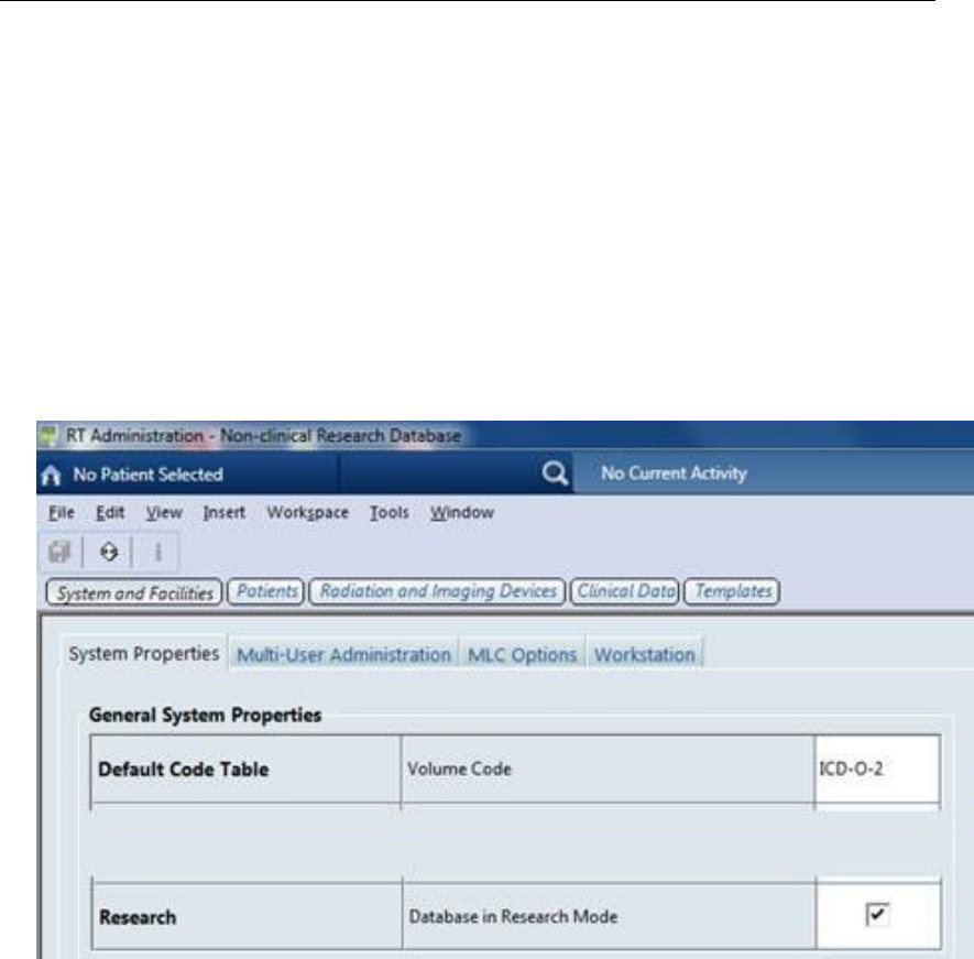
To configure an Eclipse system as an ESAPI Dev System (assuming you have the proper user
rights and the Eclipse Scripting API for Research Users license): Navigate to the RT Administration
Task using a system administrator account. Navigate to the System and Facilities workspace. Click
the System Properties tab. Click the “Database in Research Mode” flag.
See the Eclipse Scripting API Reference Guide [3] for all the details. This guide can be accessed
and downloaded by all Varian customers from MyVarian (https://myvarian.com/).
2.2.2 Developer Tools
The recommended configuration is to install your coding tools on the ESAPI Dev System. The most
useful and best supported coding tool is Microsoft Visual Studio. Many of us use Visual Studio
Professional, and there are other serious developers who use the Visual Studio Community Edition.
Other tools that should be used for serious development are source code management tools and
build / integration tools. Microsoft Team Foundation Server (TFS) and Git (https://git-scm.com/)
are 2 popular options. Serious developers also use fully automated unit testing for their clinical
software to keep future maintenance burdens low.
Debugging Plug-in Scripts
Debugging standalone executable scripts is easy - just compile a debug version of the script and run
it within the Visual Studio debugger. Debugging plug-in scripts is less obvious.
There are two usual ways to debug plug-in scripts. The first way to debug a plug-in script is to de-
velop the script within a project that uses a Plug-in Tester (https://github.com/VarianAPIs/samples/tree/master/Eclipse
Scripting API/projects/PluginTester). The Plug-in Tester is a standalone executable script that

18 Chapter 2. ESAPI basics
provides a simple window that allows the user to establish the script context and pass it to the
plug-in script. The plug-in script is modified slightly to fit into the Plug-in Tester framework. The
Plug-in tester project is compiled in debug and the user runs the Visual Studio debugger on that
project to debug the plug-in script.
The second way to debug a plug-in script is to run the script in Eclipse and attach the debugger
to the Eclipse process.
Add Automated Unit Tests for Your Scripts
ESAPIX Facades (https://rexcardan.github.io/ESAPIX/articles/facades.html) allows for known data
injection which is one way to automate your unit tests.
2.2.3 Your first script
The easiest way for the beginner to start scripting is to use the Eclipse Script Wizard to create a
Visual Studio project that can be used for developing the script.
Single File Plugin
Note that this section works on an ESAPI Dev System and will not work for a 15.1 and higher
Clinical system if script approvals are required for read-only scripts.
Select the Eclipse Script Wizard menu item from the Windows Start Menu to run the Script
Wizard. When the Eclipse Script Wizard is running, type "MyFirstSFP" and choose "Single File
Plug-in" as the script type. Choose an appropriate Destination Location for the Visual Studio
project and click the Create button.
Click "Yes" when prompted whether to launch Visual Studio after clicking Create. In the
implementation of the Execute method, add a pleasant greeting message as shown in the following
code listing.
Code 2.2
public void Execute ( S c ri ptConte x t context /* , Syste m . Windows . Window
window , Scr iptEnv i ronme n t e n vi ro nm en t */ )
{
// TODO : Add here the code that is called when the script
is launc h e d from Eclipse .
MessageB o x . Show (" Hello ␣" + context . Curre n tU se r . Name + " ,␣
loaded ␣ patient ␣ is ␣" + context . Patient . Name );
}
Save the code file and run Eclipse. Navigate to the External Beam workspace and load a patient.

2.3 ESAPI Features 19
Choose menu item Tools/Scripts, and navigate to and run the Single File Plugin script by choosing
the file "MyFirstSFP.cs" in the Eclipse Script Wizard.
2.3 ESAPI Features
2.3.1 Extract treatment planning data
ESAPI provides API methods to extract most treatment planning data that is available in Eclipse.
To gain access to the needed data, the scripter starts with the ScriptContext for plug-in scripts and
works down the object tree of the relevant object. For standalone executables, the scripter has to
establish the context through other means, either by providing chooser dialogs so that the end user
can identify and choose the relevant objects, or by implementing another scheme with a file that
lists the context(s) to work on or similar.
2.3.2 Dose and Image Profiles
Introduction
Eclipse provides tools for visualizing arbitrary dose and image profiles on planes parallel with
primary axis planes, that is either x,y, or z remain constant. Similar functionality is offered in
ESAPI without the constraint on one of the dimensions. While profiles in Eclipse serve primarily
as visualization tools they are much more potent in ESAPI. In ESAPI
1.
Profiles are precise. Profile start and end points as well as resolution are all set as parameters.
2. Profiles are easily reproducible.
3. Profiles can be oriented to match any beam geometry.
4. Profiles are readily available for calculations.

20 Chapter 2. ESAPI basics
API’s
Dose profile
Code 2.3 — Dose Profile API.
public Do s eP ro fi le G etDose P ro file ( V V e c t o r start ,
VVector stop ,
double [] pre a lloca t edBuff er );
Arguments
start 3D-profile starting point in DICOM
stop 3D-profile ending point in DICOM
preAllocatedBuffer Array of doubles
Return value
DoseProfile uniform array of dose points on a line
Dose profile API samples the 3D dose uniformly along the line segment defined with
start
and
stop
such that first point is at
start
and last point is at
stop
. Dose values are tri-linearly
interpolated at profile points.
Image profile
Code 2.4 — Image profile API.
public I m ag eP rofile Ge t ImagePr of ile ( VVector start ,
VVector stop ,
double [] pre a lloca t edBuff er );
Arguments
start 3D-profile starting point in DICOM
stop 3D-profile ending point in DICOM
preAllocatedBuffer Array of doubles
Return value
ImageProfile array of image points
Image profile API samples the 3D image uniformly along the line defined by
start
and
stop
such that first point is at start and last point is at stop.
Structure or segment profile
Code 2.5 — Image profile API.
public S e gmentPr o file Get Segmen t Profi l e (
VVector start ,
VVector stop ,
BitArray pre al locat e dBuff e r );
Arguments
start 3D-profile starting point in DICOM
stop 3D-profile ending point in DICOM
preAllocatedBuffer BitArray (boolean values)
Return value
Segment profile vector of boolean values.
GetSegmentProfile
returns an array of boolean values such that value is
true
for points
inside the segment, false otherwise.

2.3 ESAPI Features 21
Examples
Image Profile
Following function returns a triple of image profiles through isocenter in primary axis directions.
Code 2.6
public static ( I mageProfile , ImageProfile , Ima g eP ro file )
get Image Prof i lesT hroug hIso c ente r ( PlanSe t u p plan )
{
var image = plan . St r uc tu reSet . Image ;
var dirVecs = new VVector [] {
plan . S tr uc tureSet . Image . XDirection ,
plan . S tr uc tureSet . Image . YDirection ,
plan . S tr uc tureSet . Image . ZDirectio n
};
var steps = new double [] {
plan . S tr uc tureSet . Image . XRes ,
plan . S tr uc tureSet . Image . YRes ,
plan . S tr uc tureSet . Image . ZRes
};
var planIso = plan . Beams . First () . Isoc en terPo s ition ;
var tmpRes = new I m ageProfi l e [3];
//
// Throws if plan does not have ’BODY ’
//
var body = plan . Stru c tu re Set . St r uc t ur es . Single ( st => st. Id == " BODY ") ;
for ( int ind = 0; ind < 3; ind ++)
{
( var startPoint , var endP o i n t ) = Helpers .
Get S truc t ureEn tryAn dExit (
body ,
dirVecs [ ind ],
planIso , steps [ ind ]) ;
var samples = ( int ) Math . Ceiling (( endPoint - s t ar tP o in t ). Length
/ steps [ ind ]) ;
tmpRes [ ind ] = image . G et ImageP r ofile ( startPoint , endPoint , new
double [ samples ]) ;
}
return ( tmpRes [0] , tmpRes [1] , tmpR e s [2]) ;
}
Dose profile
Taking profile
Image profiles may have little use outside reporting but dose profiles on the
other hand can be leveraged for measurement comparison in beamline commissioning and quality
assurance.
Dose profile API expects profile start and stop points in DICOM, which is not usually the case
with measurements. The following example demonstrates how to sample a dose profile with start
and stop points defined in gantry system. The returned profile points have their coordinates in
DICOM but they can relatively easily be converted back. The example code only considers 4DOF
couch and patient in HFS orientation.
Converting point from gantry to DICOM involves two rotations to account for gantry and
patient support angles followed with a translation to account for isocenter.

22 Chapter 2. ESAPI basics
Code 2.7 — Transform point in gantry to DICOM.
public static VVector Ga n tryToDI C OM ( VVector point ,
double gantryInDegrees ,
double p a t ie ntSupport I nDegrees ,
VVector i s oC e n te r )
{
//
// Account for gantry
//
var retval = RotateY ( point , gant r yInDegr ee s );
//
// Account for patient s u p p o r t
//
retval = Ro t a t e Z ( retval , pat i entSu pport I nDeg r ees ) ;
//
// Add beam isoce n t er and r e a s s ig n axis ( HFS patient )
//
return new VVector ( retva l .x, - retval .z , retval .y ) + isoCenter ;
}
where rotation about Y to account for gantry is
Code 2.8 — Rotation about Y .
public static VVector RotateY ( VVector point ,
double angleInDeg ,
Direction dir = Direction . CW )
{
var a n gl eI n Ra d = angleInDe g * 2 * Math . PI / 360;
var c = Math . Cos ( angleInR a d );
var s = (( int ) dir ) * Math . Sin ( angleIn R a d );
var x = point .x * c - point . z * s ;
var z = point .x * s + point . z * c;
return new VVector (x , point .y , z) ;
}
and rotation about Z to account for patient support is
Code 2.9 — Rotation about Z.
public static VVector RotateZ ( VVector point ,
double angleInDeg ,
Direction dir = Direction . CW )
{
var a n gl eI n Ra d = angleInDe g * 2 * Math . PI / 360;
var c = Math . Cos ( angleInR a d );
var s = (( int ) dir ) * Math . Sin ( angleIn R a d );
var x = point .x * c - point . y * s ;
var y = point .x * s + point . y * c;
return new VVector (x , y , point . z);
}
To get back into gantry coordinates just invert the operations

2.3 ESAPI Features 23
Code 2.10 — DICOM to gantry.
public static VVector DI C OMToGan t ry ( VVector point , double
gantryInDegrees , d ouble pati e nt SupportIn D eg rees , VVector is o C en t er )
{
var retval = point - i so C en t e r ;
retval = new VVector ( retval .x , retval .z , - retval .y );
retval = Ro t a t e Z ( retval , - pat ientS uppor t InDeg rees ) ;
return RotateY ( retval , - g a ntryIn D egrees );
}
With tools to convert point in gantry system to DICOM, arbitrary dose profile with limits in
gantry can be extracted with
Code 2.11 — Dose profile.
public static D os eP ro fi le getBea mDoseP r ofile (
VoiBox calcu l a ti o n V ol u m e ,
Beam beam ,
VVector startInGantry ,
VVector stopInGantry ,
double s t ep Si zeInmm = 2.5)
{
//
// Convert l imits from gantry to DICOM
//
var start = Helpers . Ga n tryToDI C OM ( startInGantry , beam .
Contr o lPoints . First () . GantryAngle , beam . Con t rolPoin t s . First ()
. Patie n t Su p po rt A ng l e , beam . I socent er Posit i on );
var stop = Helpers . Gant r yToDICO M ( stopInGantr y , beam .
Contr o lPoints . First () . GantryAngle , beam . Con t rolPoin t s . First ()
. Patie n t Su p po rt A ng l e , beam . I socent er Posit i on );
var dose = beam . Dose ;
//
// Limit the re q u es t ed profile with c al culation volume
// This step can be skipped , points falling outside dose will
// be set as NaN
//
Helpers . c utWit hCalc u lati o nVolu me ( ca l c u la t i onV o l um e , ref start ,
stop - star t ) ;
Helpers . c utWit hCalc u lati o nVolu me ( ca l c u la t i onV o l um e , ref stop ,
stop - start ) ;
//
// Get the profile
//
return dose . GetDo s eProfi l e ( start , stop , new double [( int ) Math .
Ceiling (( stop - start ). L ength / s t epSizeIn m m ) ]) ;
}
If exact spacing is required,
start
and
stop
must be tweaked for profile length which is
multiple of the specified step size. This can for example be done as follows
Code 2.12 — Limit adjustment for exact spacing.
var p ro fi le Sp an = ( stop - start );

24 Chapter 2. ESAPI basics
var s p an Le n gt h = profile S pa n . Length ;
var f ullStep L ength = Math . Floor ( spanLengt h / st e pS iz eInmm ) * stepSi z eInmm ;
var adjust = st e pS iz eInmm - ( sp a n Le ng t h - full S te pLength );
profil e S pan . S caleTo U nitLen gth () ;
start = start - profil e Sp an * adj ust * 0.5;
stop = stop + pr o f il eSpan * adjust * 0.5;
, which moves both limits by the same amount. However owing to nature of floating point numbers
and calculations even adjusted limits may result in slightly off result.
Profiles may also be parameterized in terms other than start and stop positions in specified
coordinate system. The following function for example defines the profile in terms of orientation,
length, and offset from isocenter along beam axis.
Code 2.13 — Profile about beam axis.
public static D os eP ro fi le getBea mDoseP r ofile (
VoiBox calcu l a ti o n V ol u m e ,
Beam beam ,
VVector O r ie n ta t io nI n Ga n tr y ,
double p r ofileM ax Length = 600 ,
double d ista nceF r omIs ocen t erTo ward S ourc eInm m = 0,
double s t ep Si zeInmm = 2.5)
{
if ( Orie n tatio n InGan t ry . Length < 1e -8 || O r ienta t ionIn G antry .
Length > 1 e8 )
{
throw new Ar g ument E xcepti on (" Invalid ␣ direct i o n ␣ vector ␣
for ␣ profile " );
}
Orie ntatio nInGa n try . Scal e ToUnit Length () ;
var start = -( p ro fileMa xL ength * .5) * O rient a tionI n Gantr y ;
start . z += di s tanc eFro m Isoc ente rTow a rdSo urce I nmm ;
var stop = ( pr o fileMa xL ength *.5) * O rienta tionIn Gantry ;
stop . z += d i stan ceFr o mIso cent e rTow ardS o urce Inmm ;
return g etBeam D osePr o file ( calculationVo l u m e , beam , start , stop ,
stepSi ze In mm );
}
Comparing data
Reading in measurement input data is dependent on data format. For
example a simple text file of comma separated values can be read in with the following two
liner
Code 2.14 — Read in comma separated values.
var co n t e n ts = File . ReadA l lT ex t (" prof . csv " ). Trim () . Split ( ’\n ’) ;
prof3d = ( from line in c o n tent s select line . Trim ( ’\r ’) . Split ( ’ , ’) . Select
(v = > Double . Parse (v) ). ToArray () ). ToArray () ;
The code segment relies on c# feature linq to process input. The first line reads the entire content
of a text file into a single string and splits it into an array of strings at line breaks. At this point
contents
is an array of strings of comma separated values for location and measured value. Second

2.3 ESAPI Features 25
line further splits each line at commas and converts each value into double precision floating point
number, ultimately returning an array of arrays double[][]
Since calculated points are taken along a line, profile can be flattened into a function of one
argument.
Code 2.15 — Flatten profile.
public static double [][] fl a ttenPro f ile ( D os eP ro fi le profile )
{
var start = profile . Eleme n t At (0) . Position ;
return profile . Select ( pp = > new double [] {( pp . Position - start ).
Length , pp . Value }) . ToArray () ;
}
The function picks each profile point, calculates its distance from the start, and pairs it with
corresponding dose value for an entry in the flattened 1D profile.
Original 3D profile points can be recovered with two points on the original profile.
Code 2.16 — Unflatten profile.
public static ( V V e c t o r position , d o uble value ) [] unfla tt enProf ile ( double
[][] flatProfile , VVector start , VVec t o r stop )
{
var dirVec = ( stop - start );
dirVec . Sc a leToU n itLeng th () ;
return fl a tP ro fi le . Select ( val = > ( start + val [0] * dirVec , val
[1]) ) . ToArray () ;
}
Measurement data, if taken along a line, can be similarly flattened. If the start and stop points
were set with first and last measured dose values all that is required
Code 2.17 — Flatten measurement data.
var f la tP ro fi le = measur e me nt . Select ( val = > new double [] { ( new VVector (
val [0] , val [1] , val [2]) - start ). Length , val [3] }) . ToArr a y () ;
where measurement is an array of
double[4]
. First three indices, 0 through 2, are for coordinates
and the last is for measured value. If the start position was adjusted, the adjustment has to be
accounted for as on offset from zero.
With calculated and measured data in the same space comparison can be done point by point
with.
Code 2.18 — Calculate point wise difference between measured and calculated
data.
private class MyCMP : ICompare r
{
public int Compare ( objec t _a , object _b )
{
var a = _a as double [];
var b = _b as double [];
return a [0]. CompareTo ( b [0]) ;
}

26 Chapter 2. ESAPI basics
}
public static double [] d i s tanceVec ( DoseP r of il e dosePro file , d ouble [][]
measur ements , IDi f feren ceCal c ulato r d i ff C a l c )
{
//
// If me a su re ments are in 3 D flatten into 1 D.
//
var tmpMeas = m easureme n ts ;
if ( m ea surement s [0]. Length == 4)
{
tmpMeas = meas u rements . Select ( val = > new double [] {( new
VVector ( val [0] , val [1] , val [2]) - d os eP ro fi le [0].
Position ) . Length , val [3] }) . ToArray () ;
}
//
// Put m easureme n ts in in c re a si ng order on position
// along profile , per m u ta tion is r e t u r n ed in
// indices ( this is usually redunda n t )
//
var indices = E nu me r ab le . Range (0 , tmpMeas . Length ). ToArray () ;
Array . Sort ( tmpMeas , indices , new MyCMP () );
//
// Flatten dose p rofile into 1D
//
var f la tP ro fi le = flat t enProfi l e ( dos e Pr of il e );
//
// Since me a s urement points are in in c r ea si n g order ,
// we only need to march through p r o f i l e once
//
var distVec = new d o uble [ tmpMeas . Length ]. Select ( v => v = Doub le .
NaN ). T o Array ();
var p ro fi leIndex = 0;
var m e a sI n de x = 0;
foreach ( var meas in tmpMeas )
{
//
// step along profile until we have pass ed location of
// the current me a s ur em en t ( meas )
//
for (; ( p ro fi leIndex < flatProf i le . Length ) &&
( fla t Pr of i le [ pr o fi le Index ][0] < meas [0]) ; p rofileIn d ex ++) ;
//
// Have we moved beyond calcul a t ed profile , if so bail
out
//
if ( p ro fileInde x == fl a tP ro fi le . Length )
break ;
//
// Cal c u la t e distance values with provided calcu l at o r
//
distVec [ indices [ m ea s In d e x ++]] = diffCalc . C al c ul a t e ( meas ,
flatProfile , p ro fi leIndex ) ;
}
return distVec ;
}
Where diffCalc calculates the difference for the measured point in meas.
For example

2.3 ESAPI Features 27
Code 2.19 — Calculate difference between measured and calculated data.
class Poi nt Differ e nce : IDif feren c eCalc u lator
{
private double linInterp ( double v1 , double v2 , double x )
{
return (1 - x ) * v1 + x * v2;
}
private double DoseDiff ( double [] profilePoint1 , double []
profilePo i nt2 , double [] measure m en t )
{
var len = ( p r of ilePoin t 2 [0] - profil e Point1 [0]) ;
//
// de g en e ra te case , segment has zero length ,
//
if ( Math . Abs ( len ) < Double . E p s i l o n )
{
if ( Math . Abs ( profi l ePoint2 [1] - pro f il ePoint1 [1]) < Double .
Epsilon &&
Math . Abs ( m e as ur em en t [0] - pro f il ePoint1 [0]) < Double . Epsilon )
{
return p r of ilePoin t 1 [1];
}
//
// Either p r o f ile is bad , it has two v alues for
// the same argument or measu r em en t was not taken
// at the profile poi nt .
//
return Double . NaN ;
}
var x = ( m e as ur em ent [0] - pro f il ePoint1 [0]) / len ;
//
// does measu r em en t fall in segment , if not return NaN
//
if ( x < 0 || x > 1)
{
return Double . NaN ;
}
var i nterpo la tedDos e = linInter p ( pr o fi lePoint 1 [1] , p ro filePoi n t2
[1] , x );
return me a su re me nt [1] - int e rpolat e dDose ;
}
public double C a lc u la t e ( double [] measurement ,
double [][] profile , int profi l eIndex )
{
return DoseDif f ( profile . E l e me n t At ( pr o fi le In dex - 1) , profile .
ElementAt ( prof i leIndex ) , m e as ur em en t );
}
}
compares measured dose with linearly interpolated calculated value at same point. Alternatively
Code 2.20 — Unscaled 1D gamma calculator.
class Uns ca led1DG a mma : I D iffer enceC a lcula tor
{
public int N ei ghborhoo d { get ; private set ; } = 5;

28 Chapter 2. ESAPI basics
private double [] nh o od Va lu es ;
public U n scaled 1 DGamma ( int nhood = 5)
{
nhoodV a l ues = new double [( Neighb o rh oo d = nhood ) *2+1];
}
private double DotProd ( double [] v1 , do uble [] v2 )
{
return v1 . Zip (v2 , (a , b) = > (a * b) ). Aggre g a te ((a , b) =>
(a + b) );
}
//
// Short e s t dista n c e from meas u re me nt to line segment
//
private double MinDis t an ce ( double [] profilePo i n t1 ,
double [] prof i l ePoint2 ,
double [] measur e m ent )
{
//
// a = pr o filePoin t2 - pro f il ePoint1
//
var a = p rofileP o in t1 . Zip ( profilePoint2 , (av , bv ) = > ( bv
- av ) ) . ToArray () ;
//
// b = mea s ur em en t - profi l ePoint1
//
var b = p rofileP o in t1 . Zip ( measur ement , ( av , bv ) = > ( bv -
av )) . ToArray () ;
//
// | a |
//
var aNorm = Math . Sqrt ( DotProd (a , a ));
//
// | b |
//
var bNorm = Math . Sqrt ( DotProd (b , b ));
//
// a * b
//
var aDotb = DotProd (a , b) ;
//
// s calarP r ojecti o n = cos ( alpha ) * |b | = (( a* b ) /(| a|| b|)
) *| b| = ( a*b ) /|a |
//
var proj = aDotb / aNorm ;
//
// m e as ur em en t closest to s e g m e n t start ( p r of il ePoint 1)
//
if ( proj < 0)
{
return bNorm ;
}
//
// pr o je c ti on > | a| = > closest point is segment end
point ( pro f ilePoin t 2 )
//
if ( proj > aNorm )
{

2.3 ESAPI Features 29
var c = p rofileP o in t2 . Zip ( measur ement , ( av , bv )
=> ( bv - av) ). ToArray () ;
return Math . Sqrt ( DotProd (c , c)) ;
}
//
// Pr o je c ti on falls on line s e g m e n t between
profi l ePoint1 and p ro filePoin t 2;
//
return Math . Sqrt ( bNorm * bNorm - proj * proj );
}
//
// Consi d e r segme n t s in the n ei gh bo rhood of the segment i n cl u di n g
// m e as ur em en t argument .
//
public double C a lc u la t e ( double [] measuredP o i nt , double [][]
profile , int pr o fileInde x )
{
var lInd = 0;
var st a r t I nd = ( int ) Math . Max ( profi l eI nd ex - Neighb orhood
, 1) ;
var endInd = ( int ) Math . Min ( profil e In de x + Neighborhood ,
profile . Length );
endInd = Math . Max ( endInd , s t a r tIn d +1) ;
for ( var nInd = startInd ; nInd < endIn d ; nInd ++ , lInd ++)
{
nhoodV a l ues [ lInd ] = M in Di st an ce ( profile [ nInd -
1] , pr o f i l e [ nInd ] , me a su redPoin t );
}
var minVal = nho o dV al ue s . Take ( lInd ) . Min (( v ) => { return
Double . IsNaN ( v) ? Doub le . Pos it iveInf inity : Math . Abs (
v) ;}) ;
return double . I sPosit i veInf i nity ( minV a l ) ? d o uble . NaN :
minVal ;
}
}
calculates the shortest distance from a measurement point to a piecewise linear calculated
profile.
Putting it all together
With the methods in the previous paragraph extracting dose profile
and comparing it with the corresponding measurement becomes
Code 2.21
//
// ’ Me a s u red data ’ in TData . d os eP ro fi le
//
var first = TData . d os eP ro fi le . First ();
var last = TData . dos e Pr of il e . Last () ;
start = new V V e c t or ( first [0] , first [1] , first [2]) ;
stop = new VVector ( last [0] , last [1] , last [2]) ;
//
// Pick beam
//
var beam = p l an S e tu p . Beams . ElementA t (4) ;

30 Chapter 2. ESAPI basics
var cProf = Profile . g e tBeamD osePro file (
planSetup . Ge t Calcu lation Volum e () ,
beam ,
start ,
stop , 1.0) ;
//
// flatten ’ measurement ’
// note , ’ start ’ is the same point albeit in diffe r e nt co o rd i na te
// system as ’start ’ in ’ cProf ’
//
var dp = TData . d os eP ro fi le ;
var f la tP ro fi le = dp . Select ( val = > new double [] {
( new VVector ( val [0] , val [1] , val [2]) - start ). Length , val [3] }) .
ToArray () ;
//
// get vector of differe n ce s ( dista n c e is bit of misnomer , as
// the value my be signed .)
//
var dv = Helpers . dis t an ce Ve c ( cProf , flatProfile , new Unsc al ed1DGa m ma () );
Considerations
The example presented above compares measured data only to calculated
data along the measurement path. It makes no provisions for uncertainties and noise in the
measurement process which especially in high gradient areas may be enough to throw the result
off. A relatively simple way to get a handle on the uncertainties is to consider nearby dose profiles
taken for example in 3-neighborhood of the measured profile. A more robust way is compare doses
with 3D gamma index, calculation of which is beyond scope of this section.
Dose plane
Dose profiles can also be leveraged to construct rectangular dose planes by scanning in direction
of an edge of the rectangle and taking dose profiles in direction of the other. Following method
extracts an orthogonal to beam dose plane at the set offset from isocenter.
Code 2.22 — Extract orthogonal dose plane.
public static double [ ,] O rtho g onal D oseC r ossS e ction ( VoiBox calcVol ,
Beam beam ,
double i s ocente r Offset = 0,
double xSiz e I nm m = 200 ,
double zSiz e I nm m = 200 ,
double p i xe lSizeIn m m = 2.5)
{
//
// Plane X axis or i en ta ti on
//
var xDir = Helpers . Gant r yToDICO M ( new VVector (1 , 0 , 0) , beam .
Contr o lPoints . Element A t (0) . Gantr yAngle , beam . Cont ro lPoints .
ElementAt (0) . PatientSu p p or t An g le , new VVector (0 ,0 ,0) );
//
// Beam axis di r e ct i on
//
var normVec = Helpers . di r ectio nTowa r dSour ce ( beam ) ;
//
// In d iv i du al dose profile X start and end po s i ti o n s on plane
//
var start = beam . Is ocente r Posit i on - xSize * xDir * 0.5;

2.3 ESAPI Features 31
var end = beam . I socen t erPosi t ion + xDir * 0.5;
start = start + normVec * iso c enterOf fs et ;
end = end + nor m V e c * isoc e nterOf f set ;
Helpers . c utWit hCalc u lati o nVolu me ( calcVol , ref start , xDir );
Helpers . c utWit hCalc u lati o nVolu me ( calcVol , ref end , xDir );
//
// Plane Z axis or i en ta ti on
//
var zDir = Helpers . Cros s Pr oduct ( xDir , normVec ) ;
//
// These must be zero , o t h er w is e
// som e t hi n g has gone pot .
//
var a = zDir . Scal a rProduc t ( xDir ) ;
var b = xDir . Scal a rProduc t ( normVec ) ;
//
// Z limi ts
//
var zStart = beam . Isoc e nterPo s ition + nor m V e c * isoc e nterOf f set -
zDir * zSiz e * 0.5;
var zEnd = zStart + zDir * zSize ;
Helpers . c utWit hCalc u lati o nVolu me ( calcVol , ref zStart , zDir ) ;
Helpers . c utWit hCalc u lati o nVolu me ( calcVol , ref zEnd , zDir ) ;
var dose = beam . Dose ;
var xS a m p l es = ( int ) Math . Ceiling (( end - start ) . Lengt h / p i x el S i ze );
var zS a m p l es = ( int ) Math . Ceiling (( zEnd - zStart ). Length / p i xe l Si z e );
var t m p Re s ul t = new double [ zSamples * x S a m p le s ];
var ro w I n d ex = 0;
start -= zSamples / 2 * zDir * pixelSize ;
end -= zSa m p l e s / 2 * zDir * pixelSize ;
for ( double zPos = 0; zPos < z Sam p l e s ; zPos ++)
{
start += zDir * pixelSize ;
end += zDir * pix e l Si z e ;
var prof = dose . Get D os eProfil e ( start , end , new doubl e [ xSamples ])
;
//
// Rep l a ci n g NaN ’s with 0 ’s may not be smartest thing , NaN ’s are
for unknown not 0 dose
//
var pvals = prof . Select ( point => Doub le . IsNaN ( point . Value ) ? 0 :
point . Value ). ToArray () ;
Array . Cons t rained C opy ( pvals , 0 , tmpResult , rowIndex * xSamples ,
xSamples ) ;
rowIndex ++;
}
var result = new double [ zSamples , xSamples ];
Buffer . BlockCo p y ( tmpResult , 0 , result , 0 , zSamples * xSamples *
sizeof ( double )) ;
return result ;
}
If the dose plane is compared against measured data, methods described for 1D case, profile,
can be extended for 2D case.

32 Chapter 2. ESAPI basics
DVH calculation
Eclipse does not have histogram calculation for BED, EQD2 or similar derived values. For a
single plan DVH equivalent histograms can be calculated efficiently by recalculating bin limits
and re-sampling the normal DVH. However, as DVH preserves no spatial information, calculating
histogram over sum of dose values, each of which is to be independently converted, cannot be
done in this manner. Instead contributing dose matrices must be scanned separately, dose values
converted to desired representation and accumulated with other values.
The following function creates a histogram over sum of converted dose values. Dose value
conversion is passed into the function as an object argument
IDoseValueConverter converter
.
Code 2.23 — Calculate plan sum DVH for a structure.
public static ( D VHBin [] , DVHBin [] , double ) Stru c tu re DVH (
Dose [] doses ,
Structure structure ,
IDos eValue Conve r ter converter , int bins = 1024)
{
var ddvh = new int [ bins ];
//
// Add epsilon to make sure every dose value is below upper limit of
last bin .
//
var max = conver t e r . Convert ( doses . Sum (ds => ds . DoseMax3D . Dose )) +
Double . Epsilon ;
var step = max / bins ;
//
// Conta i n s structure , used to minimiz e scanned volume .
//
var b ou nd in gB ox = structure . Mesh G eo metry . Bounds ;
//
// Length of i n d iv id ua l dose profile
//
var p rofileS a mples = ( int ) Math . Ceiling ( b o undingBox . SizeX / doses
[0]. XRes ) ;
//
// number of voxels in s t r uc u tr e
//
var counter = 0;
//
// Scan in Z
//
for ( var z = bounding B ox .Z ; z < boundin g Bo x .Z + b ou nd in gBox . SizeZ ; z
+= doses [0]. ZRes )
{
//
// Scan in Y
//
for ( var y = bounding B ox .Y ; y < boundin g Bo x .Y + b ou nd in gBox .
SizeY ; y += doses [0]. YRes )
{
var start = new VVector ( b o un di ng Bo x .X, y , z ) ;
var stop = new VVector ( bou n di ng Bo x .X + boun d in g Box . SizeX , y ,
z) ;
var sumO fConv e rted D oseV a lues = new doubl e [ pr o fi leSampl e s ];
//
// Loop over ’doses ’ and accu m ul a te c o n ve r t ed dose values
//
foreach ( var dose in doses )

2.3 ESAPI Features 33
{
//
// get vector of c on v er t e d dose valu es alon g profile
//
var conv e rtedD o seVal u es = dose . G etDoseP r ofile ( start ,
stop , new double [ profi l eSample s ]) . Sel ect ( dv = >
converter . Convert ( dv . Value ) ). ToArray () ;
for ( var i ndex = 0; index < su mOfCo nvert e dDos e Valu e s .
Length ; index ++)
{
sum O fCon v erted DoseV alues [ index ] +=
conv ertedD oseVa l ues [ index ];
}
}
//
// Get s t ru c tu r e profile to d et e r mi n e whether a dose p oint
// is inside or outside of ’ structure ’
//
var s tructu re Profil e = structur e . Ge tSegme n tProfi le ( start ,
stop , new B i t Arr a y ( pr o fileSam p les ) ) . Selec t ( pro f il eP oint
=> profi l eP oint . Value ). ToArray () ;
for ( var ind = 0; ind < st r ucture P rofile . Length ; ind ++)
{
if ( true == str u ctureP r ofile [ ind ])
{
counter ++;
var bin = ( int ) Math . Floor ( s umOfC o nver t edDos eValu es [
ind ] / step );
ddvh [ bin ]++;
}
}
}
}
//
// Gener a t e output data , for differ e ntial ’DVH ’ value is divided
// by bin width ( step ) for result that is comparab l e with Eclipse .
//
var vo x e l V ol = doses [0]. XRes * doses [0]. YRes * doses [0]. ZRes * 1e -3;
var v oxelVo lO verSte p = voxelVol / step ;
var s ampleCo v erage = ( counter * v o x e lVo l / struct u r e . Volum e );
var diffDVH = new D V HBin [ bins ];
var cumDVH = new DVHBin [ bins ];
var b i n Ce n te r = step / 2;
var val = counter ;
for ( var ind = 0; ind < bins ; ind ++ , bin C e nt e r += step )
{
diffDVH [ ind ] = new DVHBin () { doseVal u e = binCenter , Volume =
ddvh [ ind ] * vo x elVolO v erStep };
cumDVH [ ind ] = new DVHBin () { doseVa l u e = binCenter , Volume = (
val -= ddvh [ ind ]) * voxelVol };
}
return ( cumDVH , diffDVH , sampl eC overage );
}
where dose converter can for example be defined as
Code 2.24 — EQD2 dose value converter.
public class EQD2 : IDos eValue Conver ter

34 Chapter 2. ESAPI basics
{
public double alpha { get ; set ; }
public double beta { get ; set ; }
public int f raction Nu mber { get ; set ; }
public double Convert ( doubl e val )
{
return val * (( val / fr a ctionNu mb er ) * ( alpha / beta ) / (2 + (
alpha / beta ) ));
}
}
where
α
and
β
are structure or organ dependent model parameters. The method scans segment and
dose volumes in two dimensions, takes profiles in third and accounts for dose values which are
inside the segment.
The method works reasonably well for large structures with relatively small number of voxels
on the structure boundary but is increasingly inaccurate with small structures. This is because the
method treats each voxel as entirely inside or outside. Consequently accuracy of the method can be
improved at the expense of computational cost by sampling the dose and structure volume at finer
resolution.
2.3.3 Automation
Starting in version 15, you can create scripts that modify RT data. With this feature, it is easy to
automate some repetitive tasks, starting from structure creation and plan generation, optimization
and dose calculation all the way to plan QA.
Writable scripts need to be approved following the institution’s guidelines. Eclipse provides a
tool to approve scripts for evaluation (where for a period of time, only certain people can run the
script). After final approval, the script is in general use. The read-only scripts can be used without
approval, or if so decided, must go through the same approval process. See Chapter 2.3.6 for details
on script approval.
A couple of things need to be present for a writable script:
The Eclipse Script Wizard in version 15.5 will create the following line for you in the main
script file, outside any namespace or class:[assembly: ESAPIScript(IsWriteable = true)]
Before the patient data is modified, this method needs to be called:
Code 2.25
Patient patient = c o ntext . Patient ;
patient . B e ginMo d ifica t ions () ;
After modification in a standalone script, this method needs to be called to save the changes:
Code 2.26
Applic a t ion app = ...
app . S a veModi ficati o ns () ;
For a plugin script, user saves the modifications in the Eclipse UI after the script has finished.
Optimization Structure Creation
Use margin function to create an optimization structure:

2.3 ESAPI Features 35
Code 2.27
Struct ur eS et ss = context . Str u ctureSet ;
if ( ss . Ca n AddStr u cture ( " CONTROL " , " PTV +5 ") )
{
Structure ptv = ss . Structu r e s . First ( st => st . Dico m T y pe == " PTV ");
Segme n tvolume segment = ptv . Margin ( ma r gi n In MM : 5) ;
Structure ne w St ructure = ss . Ad d St ru cture ( " CONTROL " , " PTV +5 ");
newStr uc tu re . Se g mentVol u me = segment ;
}
(Note that using Margin(0.0) is an easy way to copy a structure.)
With boolean functions you can modify structures further:
Code 2.28
Structure shell = ...
shell . Segme n tVolume = newStr u ct ure . Sub ( ptv );
Plan Generation
You can add a new course for the autoplanned plan setup like so:
Code 2.29
Course course ;
if ( patient . Courses . Where (x = > x. Id == " AutoPl a n ") . Any () )
{
course = pa t i e n t . Courses . Where (x = > x. Id == " Auto P l a n ") . Single () ;
}
else
{
course = c urpat . AddCourse () ;
course . Id = " AutoP l a n ";
}
Add a new plan setup:
Code 2.30
Exte r nalPl a nSetup eps = course . A d dExte r nalPl a nSetu p ( ss );
eps . Id = " A utoPlanV M AT ";
Add beams. Note that ESAPI gives options to add VMAT beams or IMRT beams, but those are
meant to be used when you already have an optimized plan from your own optimizer, and you want
to import that to Eclipse (for e.g. dose calculation). When you plan to run optimization, add normal
arc fields or static open fields (as you would do in Eclipse UI).
Code 2.31
VVector i s oc e n te r = new VVector ( Math . Round ( ptv_hig h . Cen t e rP oi nt .x / 10.0
f) * 10.0 f , Math . Round ( ptv_high . Cente r P oi nt .y / 10.0 f ) * 10.0 f , Math .
Round ( ptv_high . C en te rP oi nt .z / 10.0 f ) * 10.0 f);
var ebmp = new Ext erna l Beam M achi n ePar amete rs ( " Truebeam " , "6X ", 600 , " ARC

36 Chapter 2. ESAPI basics
" , null ) ;
Beam vmat1 = eps . AddArc B ea m ( ebmp , new VRect < double >( -100 , -100 , 100 ,
100) , 30 , 181 , 179 , G an tryDir e ction . Clockwise , 0 , isocen t e r );
Beam vmat2 = cureps . AddAr c Be a m ( ebmp , new VRect < double >( -100 , -100 , 100 ,
100) , 330 , 179 , 181 , Gant r yDirec t ion . Co u n t erCl o c k w ise , 0, isocente r );
or
Code 2.32
Beam imrt1 = eps . Add S ta ticBeam ( ebmp , new VRect < double >( -100 , -100 , 100 ,
100) , 0 , 90 , 0, isocenter );
Fit the collimator to the target and set calculation model and dose prescription:
Code 2.33
vmat1 . Fit Colli mator T oStr u cture ( new FitT o Struc tureM a rgins (10) , ptv_low ,
true , true , false ) ;
eps . S e tCalc u latio n Model ( Ca lc ulatio n Type . Photon V M AT Op ti mization , "
PO_15014 " );
eps . S e tPresc r ip tion ( NFractions , new DoseValue (2 , " Gy ") , 1) ;
DVH Estimation
You can create optimization objectives for the plan easily using RapidPlan. If you have suitable
RapidPlan models available in the system, use the method CalculateDVHEstimates() to run esti-
mation. Two dictionaries need to be set up before the function call. These are the same steps you
normally do in the DVH Estimation user interface: map dose levels to the target structures, and
match plan structure IDs to the ones used in the RapidPlan model.
Code 2.34
Dictionary < string , DoseValue > leve ls = new Dictionary < string , DoseValue
>() ;
levels . Add ( ptv50 . Id , new DoseValue (50 , " Gy ")) ;
levels . Add ( ptv70 . Id , new DoseValue (70 , " Gy ")) ;
Dictionary < string , string > ma t c h e s = new Dictionary < string , string >() ;
matches . Add ( ptv70 . id , " PTV_High " );
matches . Add ( ptv50 . id , " PTV_Low ") ;
eps . S e tCalc u latio n Model ( Ca lc ulatio n Type . D V HEstimation ,
DVH E stima tionA l gorit hm );
eps . C a lcula teDVH E stima tes ( m odelId : " Prostat e " , t argetD o seLeve ls : levels ,
stru c tureMa tc hes : matches );
After a successful calculation, the optimization objectives are automatically added to the plan.
The estimate curves for upper and lower bound can be found in ExternalPlanSetup.DVHEstimates
property.

2.3 ESAPI Features 37
Optimization
If you haven’t used RapidArc to create optimization objectives automatically, you must set DVH
objectives before starting the optimization.
ExternalPlanSetup has a property OptimizationSetup that gives you access to objectives:
Code 2.35
Structure ptvLo w O pt = ...
eps . O p timiza tionSe t up . A ddPoin tO bject i ve ( ptvLowOpt ,
Opt i miza tionO bjec t iveO p erat o r . Lower , new DoseValue (
doseob j e ctivevalue _l o w , " Gy ") , 100 , 100) ;
eps . O p timiza tionSe t up . A ddPoin tO bject i ve ( ptvLowOpt ,
Opt i miza tionO bjec t iveO p erat o r . Upper , new DoseValue (
dos e objec tivev a lue_l ow +3.0 f , " Gy ") , 30 , 50) ;
eps . O p timiza tionSe t up . A ddNo r malTi ssueO bject i ve (80.0 f, 0.0f , 100.0 f, 40.0
f , 0.05 f ) ;
Already existing objectives can be found in ExternalPlanSetup.OptimizationSetup.Objectives.
Iterate through them like this:
Code 2.36
foreach ( var objective in eps . Op t imizat i onSet u p . Obje c ti v es . OfType <
Optim i zationP o in tObject i ve >() )
{
...
}
And similarly for other types of objectives. If you don’t use the OfType extension (or cast the type
in some other way), you get a list of objects of a base type that does not show all the properties that
the object has.
There is also ExternalPlanSetup.OptimizationSetup.Parameter for fluence smoothing etc.
After setting the objectives you can call the optimization function:
Code 2.37
eps . S e tCalc u latio n Model ( Ca lc ulatio n Type . Photon V M AT Op ti mization ,
Opt i mizat i onAlg orith m );
eps . Op t im izeVMAT () ;
or
Code 2.38
eps . S e tCalc u latio n Model ( Ca lc ulatio n Type . Photon I M RT Op ti mization ,
Opt i mizat i onAlg orith m );
eps . Optimize ();
Optimize() has also variants where you can define the maximum number of iterations, continue
optimization, or intermediate dose.

38 Chapter 2. ESAPI basics
Leaf sequencing
Leaf sequencing for IMRT fields is run by calling
Code 2.39
eps . C a lcula teLeaf Motio n s () ;
This version uses the LMC options that are found in the plan (most often the default LMC options).
If you want to overrun those, you can use other versions of the method, for example:
Code 2.40
eps . S e tCalc u latio n Model ( Ca lc ulatio n Type . PhotonLeafMotion s ,
Lea f Motio n Calcu l ator );
eps . C a lcula teLeaf Motio n s ( new S martLMC Op tions ( true , false )) ;
This defines that the algorithm to be used is SmartLMC, and the field borders should be fixed, and
jaw tracking not used. Other options you can use are LMCVOptions and LMCMSSOptions.
MCO
After optimaztion, the trade-off exploration context of PlanSetup (eps.TradeoffExplorationContext)
can be used for Multicriteria Optimization (MCO).
Code 2.41
// Retrieve trade - off canfid a t es
var t radeo f fCandi da te = eps . T r adeo f fExp l orat i onCon text .
Tra d eoff S truc tureC andid ates ;
...
// Add stur c tu r es into trade - off object i ve s
eps . T radeo ffExp lorat ionCo n text . A d dTrad e offOb jecti v e ( sturct u r e );
...
// Create plan collec t i on
if ( eps . Tra d eoffE xplor ation Conte xt . C anCr e atePl anCol l ecti o n )
{
eps . T radeo ffExp lorat ionCo n text . C r eateP l anCol lecti o n ( false ,
Tra deof fPla n Gene rati o nIn t erme diat e Dos e Mode . NotUsed ) ;
}
// Navigate with the trade - off object i v es
var cost = eps . Trad eoffE xplor ation Conte xt . G etObje c tiveCo st (
trad e offOb j ective );
var l o we rL i mi t = eps . Tra deoff Explo ratio nCont ext . Get O bjec t iveLo w erLi m it (
trad e offOb j ective );
var u p pe rL i mi t = eps . Tra deoff Explo ratio nCont ext . Get O bjec t iveUp p erLi m it (
trad e offOb j ective );
var n ewRest ri ctorPo s = cost + ( uppe r Li mi t - lowerL i mi t ) * 0.5;
eps . T radeo ffExp lorat ionCo n text . S etObj ectiv eUppe rRest ricto r (
tradeoffObject i v e , n ewRest r ictorP o s );
eps . T radeo ffExp lorat ionCo n text . Se t ObjectC o st ( trade o f f Ob j e ct i v e ,
cos t ForT r adeof fObje ctive );
...
// Save and ap ply
eps . T radeo ffExp lorat ionCo n text . A pplyT rade o ffEx p lora tionR esul t () ;
app . S a veModi ficati o ns () ;

2.3 ESAPI Features 39
Dose Calculation
Calling the dose calculation is simple:
Code 2.42
eps . S e tCalc u latio n Model ( Ca lc ulatio n Type . PhotonVolumeDose ,
Dos e Calc u latio nAlgo rithm );
eps . Ca l culateD o se () ;
There is also a version of calculating dose with "Fixed MUs":
Code 2.43
var p re se tValues = new List < KeyValuePai r < string , MetersetValue > >() ;
preset Va lu es . Add ( new KeyValuePair < string , MetersetVal u e >( field1 .Id , new
Meter s etValue (100 , Dosim e te rUnit . MU )) );
eps . C alcul ateD o seWi t hPre s etVa lues ( pres e tValues ) ;
Note that this version only takes the preset values into account, when the field in an IMRT field.
(For other types of fields, you can easily set the MUs by adjusting the field weight after dose
calculation. The relation between field weight and field MUs is linear.)
Verification Plan Creation
When creating a verification plan, you typically want to recreate the plan on a phantom image. The
first step is to copy the image from a phantom patient to the current patient. After that you use a
special method to create the verification plan.
The first ’null’ in the sample below is a place where you can put target study, if you have one
already that you want to use. The second ’null’ is a place where you can specify the study id under
which the image can be found. If the image id itself is unique under the phantom patient, the study
id is not needed.
Code 2.44
string error ;
if ( pat . Can C opyI m ageF r omOt h erPa tient ( null , " Ph a ntomPat i ent " , null , " CCI -
image " , out error ) )
{
var phan t omStr u cture S et = pat . C o pyIm a geFro mOthe rPati ent ( " UITScript -
Breast " , null , " CCI - image ");
var v erific at ionPla n = context . Course .
Add Exte r nalP lanS e tupA sVer ific a tion Plan ( phant o m St r uc t ur e Se t , eps );
}

3. DICOM basics
REX CARDAN, PHD
3.1 Introduction
Digital Imaging and Communications in Medicine (DICOM) is the fundamental data storage and
communication method in medical applications. In radiation oncology, CT images are taken and
sent (via DICOM transport) to the planning system. DICOM structure sets encapsulate the CT set
with segmented voxel information. A DICOM plan is created and sent to an accelerator which can
process the file and deliver to a patient. DICOM RT images are acquired to make sure the patient is
aligned and DICOM treatment records are stored to ensure the patient receives the correct radiation
dose. In summary, DICOM is everywhere in our field and scripters need to be very familiar with its
application and its design.
3.1.1 DICOM Structure
A DICOM file is a custom designed binary format. The technical specifications of the format are
listed in a long (and riveting) DICOM standard set of documents (https://www.dicomstandard.org/current/).
The basic idea is there is an outermost DICOM object which contains snippets of information called
DICOM elements. The DICOM element is the fundamental building block of DICOM objects.
Each element contains 3 main parts : an ID called a tag, a data type called a value representation
(VR), and the actual data.
3.1.2 DICOM Tag
The ID (Tag) is a hexadecimal identifier for each element. Each hexadecimal is two charac-
ters long (00,01,..FF). The first two hexadecimal values represent the group ID and the last
two values are the element ID within the group. For example, in the following image you can
see the elements of a DICOM CT slice. In particular, I have highlighted the element Trans-
fer Syntax UID (0002, 0010) with the group ID 0x00,0x02 and the element ID 0x00,0x10.

42 Chapter 3. DICOM basics
3.1.3 Value Representation
The value representation or VR is the data type for the element. It is synonymous with string, int,
long, etc. in programming languages but with a richer variety. The full list of VR types supported
in the newest DICOM Standard are listed below. One of the VRs is the sequence type which allows
nesting of DICOM elements. It is similar to a List<T> or Array type in .NET. When a DICOM
object contains sequence elements, the structure resembles a tree structure, a list of lists, like XML.
VR types are either explicitly set in the element (called Explicit Little/Big Endian syntax) or they
are known implicitly by the element ID. For example, the DICOM element Transfer Syntax UID
is always of VR type Unique Identifier. The program or library used to read DICOM files must
contain a DICOM dictionary to be able to look up VRs based on the elements DICOM Tag if it is
not explicitly provided.
Available VR types in DICOM Standard 2017c. From Table 6.2-1 in The DICOM Standard
Part 5
• Application Entity
• Age String
• Attribute Tag
• Code String
• Date
• Decimal String
• Date Time
• Floating Point Single
• Floating Point Double
• Integer String
• Long String
• Long Text
• Other Byte
• Other Double
• Other Float
• Other Word
• Person Name
• Short String
• Signed Long
• Sequence Long
• Signed Short
• Short Text
• Time
• Unlimited Characters
• Unique Identifier
• Unsigned Long
• Unknown

3.2 Exploring DICOM Visually 43
• Universal Resource Identifier
• Unsigned Short
• Unlimited Text
3.1.4 DICOM Data
The real meat of each DICOM element is of course the data. The data portion of the element must
be decoded based on the VR. If the VR is Code String for example, the data must be decoded as
a string. The data section can actually hold multiple values of the VR type. In this sense, almost
every element is like an array. Most elements just hold one datum, but if there are multiple values
(called value multiplicity greater than one), then the data will be separated by the ’/’ character.
3.2 Exploring DICOM Visually
If you would like to get a understanding of the layout of a DICOM object, the best thing to do is
open up the file in DICOM tool. My personal favorite and lightweight application is called "Sante
Hexidecimal Viewer". This viewer provides element inspection with a tree view to see the positions
of various DICOM elements within the file. Additionally, it allows inspection of the actual bytes
which can aid in debugging DICOM problems.
3.3 Exploring DICOM With Evil DICOM
Because DICOM files are specially formatted binary files, you won’t be able to just open one in
your favorite text editor. Instead to inspect and manipulate them, you will need to grab a DICOM

44 Chapter 3. DICOM basics
library. There are some great libraries including PyDICOM, fo-dicom, dcmtk, and my personal
favorite, Evil DICOM. Since I am most familiar with Evil DICOM, the following examples will use
this .NET library to demonstrate the principles needed when programming against DICOM files.
3.3.1 Installing EvilDICOM via NuGet
1. Create a new C Sharp .NET console project. 2. Right click your project and choose Manage
NuGet Packages 3. Search for "EvilDICOM" and choose install to automatically pull the library
from the internet
3.3.2 Opening Your First DICOM File
If you don’t have any DICOM files available, export some from Eclipse to your desktop. DICOM
files typically end with ".dcm" extension and begin with letters which signify their file type (Varian
convention). The most common file types are :
• "RP..." - RT Plan object
• "RD" - RT Dose object
• "RS" - RT Structure Set object
• "RI" - RT Image Object (DRR, kV, Portal image)
• "CT" - Computed Tomography Image Slice
• "PT" - Positron Emission Tomography Image Slice
• "MR" - Magnetic Resonance Image Slice
• "REG" - Registration Object
Choose a file that you want to inspect and copy the path. In Windows, to copy the path, hold
shift when right clicking the file and choose "Copy as Path" option. To load the DICOM object into
memory so you can inspect it, use the following code:
Code 3.1 — Read DICOM object from file.
// Your copied path below
var path = @ " \\ vms - image \ va_data$ \ DICOM \ CT .1. dcm " ;
var ctSlice = D IC OM Object . Read ( path );

3.3 Exploring DICOM With Evil DICOM 45
A CT image slice object has many different elements which define the image. It contains the
mA, kVp and relevant equipment parameters used to acquire the scan. It also contains the current
window/level, position in 3D space and all of the voxels in the image. To see all of the elements,
you can access the Elements property.
Code 3.2
var el e m e n ts = c t S l i c e . Elements ;
foreach ( var el in elements )
{
Console . Writ e L in e ($ "Tag ={ el . Tag }") ;
Console . Writ e L in e ($ "VR ={ el . VR }") ;
Console . Writ e L in e ($ " Data ={ el . DData } ");
}
3.3.3 Selecting Elements And Accessing Data
The DICOM elements can be selected by tag ID in most libraries. The DICOM element tag is a
unique set of 4 bytes which identifies the element and gives its data meaning. The first 2 bytes
are the DICOM group ID, and the last 2 bytes are the element ID. The bytes are typically shown
in hexadecimal notation. For example, the DICOM element tag which holds the patient ID is
(0010,0020), where the group ID is 0x00,0x10 and the element ID is 0x00,0x20. To select the
patient ID in our DICOM object, you would do the following:
Code 3.3
var p atient Id Elemen t = ctSlice . Fin d F ir s t (" 00100020 ") ;
var p a t ie n tI d = ( stri ng ) pat ie ntIdEl em ent . DData ;
All public DICOM element tags are defined in Part 6 of the DICOM standard (http://dicom.nema.org/medical/dicom/current/output/pdf/part06.pdf).
You will need to spend the next few days memorizing all of the thousands of the DICOM tags. Go
ahead and pause your progress in the book and come back when you are finished. Still reading? Of
course, for those who are lazy (hint: you), there are a lot of helper methods to make it easy to select
elements without knowing the tag.
3.3.4 The Tag Helper
The first way you can access tag IDs is to use the
TagHelper
class found in EvilDICOM.Core.Helpers
namespace. The tag helper just finds the ID using static strings of the name of the element. For
example, to find the Patient Id element you can write:
Code 3.4
var p atient Id Elemen t = ctSlice . Fin d F ir s t ( TagHelper . Patient I D )
;
var p a t ie n tI d = ( stri ng ) pat ie ntIdEl em ent . DData ;
3.3.5 The Selector Class
The next method of selection is my personal favorite. If you look at the previous example, you
finding an element through an interface of IDICOMElement which has properties called
DData
and
DData_
. These are just holders for data but the type is unknown. Because of this, a cast must
be performed. Evil DICOM has a neat way to strongly type the data so you can take advantage

46 Chapter 3. DICOM basics
of the compiler checks in Visual Studio. The magic trick is the class called DICOMSelector. The
DICOMSelector class is like the TagHelper class in that it has properties for each DICOM element
in part 6 of the standard. But unlike the selection we did before, the elements selected by the
DICOMSelector class contain properties
Data
and
Data_
which are strongly typed. To select with
this method, you call the GetSelector() method on a DICOM object as follows:
Code 3.5
var se l e c t or = c t S l i c e . Get S el ec to r () ;
var p a t ie n tI D = selector . P a t ie n tI D . Data ;
3.3.6 DICOM Data
DICOM elements can hold one or more datum of the type specified by the VR. If you are wanting
to inspect just the first datum or if you believe only one datum value is present, you use the
Data
property as we saw in the above example. However, if you want to inspect or manipulate multiple
values, you must use the
Data_
(with a trailing underscore) in Evil DICOM. For example, the
position of a CT image slice is stored in element (0020,0032) - Image Position. The data is an array
of 3 values : X, Y, and Z location. You can access these values in the following way:
Code 3.6
// Notice underscor e
var po s i t i on = selector . I m agePosi t io n . Data_ ;
var x = p o s i t ion [0];
var y = p o s i t ion [1];
var z = p o s i t ion [2];
3.3.7 Working With Sequences
Sequences are elements which contain more elements. However, a sequence’s children are not
DICOM elements. They are Sequence Items. A sequence item can be thought of as another DICOM
object in that it is just a collection of elements. So a sequence then is just a container for descendant
DICOM objects. This hierarchy can be seen in the diagram below. Sequences are very important in
3.3.8 Hacking DICOM Files
So far we have only been concerned with reading DICOM files, but you can also change data and
write new hacked files. For example, if you wanted to changed the patient name and ID, you could
execute:
Code 3.7
var se l e c t or = c t S l i c e . Get S el ec to r () ;
selector . Patient N a me . Data = " FLINST O N E ^ FRED ";
selector . P at i en t I D . Data = " 123456 ";
ctSlice . Write ( path );
3.4 Conclusion
This chapter has been a review of the DICOM structure and some tools to get started programming
against DICOM files. Having established a foundational understanding of the DICOM file format,
we can extend our journey into the more complex networking operations.

4. Daemons : A tour through Varian’s DICOM API
REX CARDAN, PHD
4.1 Introduction
DICOM network operations are the backbone of a radiation oncology operation. Files are
searched, moved, stored all in an advanced protocol defined in Part 7 of the DICOM standard
(https://www.dicomstandard.org/current/). The network nodes which are sending and receiving
DICOM messages are often referred to as DICOM daemons (pronounced demons). The commu-
nication is a special DICOM specific language layered on TCP/IP protocol. In this chapter, we
will learn the language of the daemons allowing for some very advanced clinical and research
operations.
DICOM Service Classes
Typically DICOM nodes on the network are referred to as service class users (SCU) or service class
providers (SCP). SCUs are the clients who are usually initiating calls and the SCPs are responding
to the calls and sending back the data requested. All DICOM services have an identity on the
network consisting of 3 main properties: IP address, communication port, and application entity
title (AE title). These unique properties allow for secure transmission of data on a network. Most
commercial SCPs will have a white-list of services to which they are allowed to communicate. Any
request coming from entities not listed in the white-list is considered hostile and calls will not be
answered.
Source Code
The source code from this chapter is available on Github in the VarianAPIs repositories. The web
address is
https://github.com/VarianAPIs/DICOM_Communication_101
. The solution file
contains each example with a program class that runs the requested tutorial. Site specific details
will have to be modified (IP addresses, etc) for it to work properly.

48 Chapter 4. Daemons : A tour through Varian’s DICOM API
4.2 Setting Up a Varian Daemon
Before we get to exploring the communication details, we need to set up our Varian DICOM
environment. The provided SCP (called the daemon from here on) is a software installation separate
from Aria and Eclipse. In versions prior to Aria 15, the DICOM daemon could be installed on any
Eclipse thick client workstation. In versions 15 and higher, the DICOM services all run from a
single server. This tutorial will cover the setup principles of the DICOM daemon which will work
with all Aria versions. However the images and exact steps will be taken from the setup in version
15.5.
4.2.1 Finding the DICOM Services Server
You will need administrative rights to be able to proceed through this tutorial, and mis-configuring
or changing existing DICOM services can be very bad. The DICOM services server can be found
from the Varian Service Portal (web service). From there, go to
Inventory » Workstation Details
.
There you will find a list of all Varian servers and workstations on your network. Search for the one
that has the "DCM" in the name. This is the server you will remote desktop (RDP) into in order to
configure the daemon. One you RDP into the DICOM services server:
1. Type Windows + Q to open the Windows search
2. Enter the text "DICOM ser..."
3. Select DICOM Services Configuration

4.2 Setting Up a Varian Daemon 49
4.2.2 Spawning a Daemon
1. Select Add Service
2. Select Database Service
3. Set the AE Title, port number, and record the IP address from the ethernet adapter.
4. Check Automatic Patient Creation
5. Select Add New (trusted entity)

50 Chapter 4. Daemons : A tour through Varian’s DICOM API
4.2.3 Adding a Trusted Entity
This next step is site specific. You will need to whitelist some computers so that they can talk to
the daemon. For each computer that will need to communicate with the daemon, you will have to
add a new trusted entity. The AE title just needs to be a unique name for the DICOM nodes. The
IP address will be the address for the computer from which you will be calling (probably where
Visual Studio is installed). Remember the port that you assign here. It will be important for some
operations.

4.3 DICOM Language Basics 51
We are now ready to start communicating. The Varian daemon can perform several useful operations
for a client. Each of the operations is explored in the following sections.
4.3 DICOM Language Basics
The exact bitwise operations of the protocol are beyond the scope of this chapter. Instead we will
focus on high level communication concepts more relevant to the DICOM library user. If instead,
you were trying to develop a library or implement a DICOM call from scratch, I recommend
the book Digital Imaging and Communications in Medicine (DICOM): A Practical Introduction
and Survival Guide by Pianykh. Additionally, the DICOM transport layer documentation (part 8)
provides very detailed information. For the purposes of learning DICOM communication using
an existing library, we will continue to use Evil DICOM. For details on setting up a project with
Evil DICOM, see the previous chapter. The main DICOM calls we are interested in here are the
following:
• C-ECHO (DICOM "ping")
• C-FIND (DICOM search)
• C-MOVE (DICOM move and storage)
• C-STORE (DICOM storage)
4.3.1 C-ECHO
The first network operation is the simplest. When starting to set up a DICOM network, the DICOM
creators designed a mechanism equivalent to the ping command in Windows. Successful execution
of the following command ensures that 1) the DICOM node is up and running and 2) it is allowed
to communicate with the client.

52 Chapter 4. Daemons : A tour through Varian’s DICOM API
Code 4.1
// Store the details of the daem on ( Ae Title , IP , port )
var daemon = new Entity (" PHYSX_ D IC OM " , " 10.22.8 6 .6 4 " , 51 402) ;
// Store the details of the clie nt ( Ae Title , port ) -> IP a d d ress is
determin e d by Crea t eL oc al () method
var local = Ent i ty . Creat e Lo ca l (" DICOM E C 1 " , 9999) ;
// Set up a client ( DICOM SCU = Service Clas s User )
var client = new DICOM S C U ( loca l ) ;
// TRY C - ECHO
var canPing = client . Ping ( daemo n );
// Write results to console
Console . Writ e L in e ($ " DICOM ␣C - Echo ␣ from ␣ { local . AeTitle } ␣=> ␣" + $ "{ daemon .
AeTitle }␣ @{ daemon . IpAddre s s }:{ daemon . Port } ␣ was ␣ succes s fu ll ?␣ { canP i n g }
") ;
Console . Read () ; // Stop here
4.3.2 C-FIND
The C-FIND operation allows searching patient DICOM files using certain keys such as patient Id,
SOP instance UIDs, etc. Typically, unless you know SOP UIDs, you will need to start with the
patient Id and work your way down from studies to series, and then from series to images. The
convention in DICOM is to refer to any DICOM file as a DICOM "image". This will include RT
plans, dose files, and structure sets as well as actual image data. If you know the patient Id, then
you can use the following technique to find all studies, series and images.
Code 4.2
// Store the details of the daem on ( Ae Title , IP , port )
var daemon = new Entity (" PHYSX_ D IC OM " , " 10.22.8 6 .6 4 " , 51 402) ;
// Store the details of the clie nt ( Ae Title , port ) -> IP a d d ress is
determin e d by Crea t eL oc al () method
var local = Ent i ty . Creat e Lo ca l (" DICOM E C 1 " , 9999) ;
// Set up a client ( DICOM SCU = Service Clas s User )
var client = new DICOM S C U ( loca l ) ;
// Build a finder class to help with C - FIND o p e ra ti on s
var finder = client . Get C F in d er ( daemon );
var studies = finder . F in dS tu di es (" D A 0 0 0 0 1 ") ;
var series = finder . Fin d S er i es ( studies ) ;
var images = finder . Fin d I ma g es ( series );
// Write results to console
Console . Writ e L in e ($ " DICOM ␣C - Find ␣ from ␣ { local . AeTitle } ␣=> ␣" +
$" { daemo n . AeTitle }␣ @{ daemon . IpAdd r e ss }:{ daemo n . Port }: ");
Console . Writ e L in e ($ "{ studies . Count () } ␣ Studies ␣ Found ");
Console . Writ e L in e ($ "{ series . Count () }␣ S eries ␣ Found ") ;
Console . Writ e L in e ($ "{ images . Count () }␣ I mages ␣ Found ") ;
Console . Read () ; // Stop here
4.3.3 C-MOVE
Finding DICOM files is great, but you typically want to do something with those results. Enter C-
MOVE. The C-MOVE operation is used to take results from a C-FIND and send them to a DICOM
node on the network (which can be the same as the DICOM node you are calling from). At UAB,

4.3 DICOM Language Basics 53
we use this technique to rapidly send patient DICOM files to Mobius 3D for rapid commissioning
of the system. You can also send DICOM files to a PACs or even back to Aria. The following
example shows how to move to a separate destination (Mobius in this case).
Code 4.3
// Store the details of the daem on ( Ae Title , IP , port )
var daemon = new Entity (" PHYSX_ D IC OM " , " 10.22.8 6 .6 4 " , 51 402) ;
// Store the details of the mobi us DICOM entity ( Ae Title , IP , port )
var mobius = new Entity (" MOBIUST " , " 10.241 . 20 .4 1 " , 104) ;
// Store the details of the clie nt ( Ae Title , port ) -> IP a d d ress is
determin e d by Crea t eL oc al () method
var local = Ent i ty . Creat e Lo ca l (" DICOM E C 1 " , 9999) ;
// Set up a client ( DICOM SCU = Service Clas s User )
var client = new DICOM S C U ( loca l ) ;
// Build a finder class to help with C - FIND o p e ra ti on s
var finder = client . Get C F in d er ( daemon );
var studies = finder . F in dS tu di es (" D A 0 0 0 0 1 ") ;
var series = finder . Fin d S er i es ( studies ) ;
// Filter series by modality , then create list of
var plans = ser i es . Where ( s => s . Modality == " RTP L AN " )
. Sele c t Ma ny ( ser = > finder . Fin d I ma ge s ( ser )) ;
var doses = ser i es . Where ( s => s . Modality == " RTD O SE " )
. Sele c t Ma ny ( ser = > finder . Fin d I ma ge s ( ser )) ;
var cts = series . Where ( s => s. Mod a l i t y == " CT ")
. Sele c t Ma ny ( ser = > finder . Fin d I ma ge s ( ser )) ;
var mover = cli e nt . GetCMover ( daemon );
ushort msgId = 1;
foreach ( var plan in plans )
{
Console . Writ e L in e ($ " Se n d i n g ␣ plan ␣ { plan . SOP In stanceU ID }... " );
// Make sure Mobius is on the whit e l is t of the daemon
var re s p o n se = mover . Sen d C Mo v e ( plan , mobius . AeTitle , ref msgId ) ;
Console . Writ e L in e ($ " DICOM ␣C - Move ␣ Results ␣ : ␣") ;
Console . Writ e L in e ($ " Number ␣ of ␣ Comp l e te d ␣ Ope r a ti on s ␣: ␣{ response .
Num b erOfC o mplet e dOps }") ;
Console . Writ e L in e ($ " Number ␣ of ␣ Failed ␣ Op e r at i on s ␣:␣ { response .
Numb e rOfFa i ledOps }" );
Console . Writ e L in e ($ " Number ␣ of ␣ Rema i n in g ␣ Ope r a ti on s ␣: ␣{ response .
Num b erOfR e maini n gOps }") ;
Console . Writ e L in e ($ " Number ␣ of ␣ Warning ␣ Operation s ␣: ␣{ response .
Numb erOfWa r ningO p s }" );
}
Console . Read () ; // Stop here
4.3.4 C-MOVE To Self
Of course a lot of times, you just want to get the DICOM files to do something with them. You
can actually instruct the daemon to move to the client node. It is a little trickier to do this because
you will need to create a separate "receiver" to catch the files when they come back. Because these
two nodes will need to run at the same time, they will need to be run on two separate threads.
Evil DICOM will help you manage the threading part if you are using that library. The following
example shows how to setup a DICOM service class provider to catch the files as they get sent back
to the client.

54 Chapter 4. Daemons : A tour through Varian’s DICOM API
Code 4.4
// Set up a r e c eiv e r to catch the files as they come in
var re c e i v er = new DICOMSCP ( local );
// Let the daemon know we can take anything it sends
receiver . Sup p orte d Abst r actS y ntaxe s = Abs t ra ctSynta x .
ALL _ RADI O THERA PY_ST ORAGE ;
// Set up storage l ocat i o n
var d es kt op Pa th = Enviro n me nt . Ge tF ol derPath ( Env i ro nm en t . Spe c ia lFolder .
Desktop );
var s to ra ge Pa th = Path . Combine ( desktopPath , " DICOM ␣ S t o r age ");
Directory . Cre at eDirec t ory ( s to ra ge Pa th );
// Set the action when a DICOM files comes in
receiver . DIMSES e rv ic e . CSt or eServic e . C S toreP a yload A ction = ( dcm , asc ) = >
{
var path = Path . Combine ( storagePath , dcm . GetSele c to r ().
SOPI n st anceUID . Data + ". dcm " );
Console . Writ e L in e ($ " Wr i t i n g ␣ file ␣ { path }... ") ;
dcm . Write ( path );
return true ; // Lets daemom know if you su c ce ss fully wrote to drive
};
receiver . Lis tenFo rInco ming A ssoc i atio n s ( true ) ;
C-MOVE To Self : Full Example
To send to yourself (the initiating client), simply change the AE title in the mover.SendCMove(..)
method to the local entity title. The full example of this process can be seen in the following
code,
Code 4.5
// Store the details of the daem on ( Ae Title , IP , port )
var daemon = new Entity (" PHYSX_ D IC OM " , " 10.22.8 6 .6 4 " , 51 402) ;
// Store the details of the clie nt ( Ae Title , port ) -> IP a d d ress is
determin e d by Crea t eL oc al () method
var local = Ent i ty . Creat e Lo ca l (" DICOM E C 1 " , 9999) ;
// Set up a client ( DICOM SCU = Service Clas s User )
var client = new DICOM S C U ( loca l ) ;
// Set up a r e c eiv e r to catch the files as they come in
var re c e i v er = new DICOMSCP ( local );
// Let the daemon know we can take anything it sends
receiver . Sup p orte d Abst r actS y ntaxe s = Abs t ra ctSynta x .
ALL _ RADI O THERA PY_ST ORAGE ;
// Set up storage l ocat i o n
var d es kt op Pa th = Enviro n me nt . Ge tF ol derPath ( Env i ro nm en t . Spe c ia lFolder .
Desktop );
var s to ra ge Pa th = Path . Combine ( desktopPath , " DICOM ␣ S t o r age ");
Directory . Cre at eDirec t ory ( s to ra ge Pa th );
// Set the action when a DICOM files comes in
receiver . DIMSES e rv ic e . CSt or eServic e . C S toreP a yload A ction = ( dcm , asc ) = >
{
var path = Path . Combine ( storagePath , dcm . GetSele c to r ().
SOPI n st anceUID . Data + ". dcm " );
Console . Writ e L in e ($ " Wr i t i n g ␣ file ␣ { path }... ") ;
dcm . Write ( path );
return true ; // Lets daemom know if you su c ce ss fully wrote to drive
};
receiver . Lis tenFo rInco ming A ssoc i atio n s ( true ) ;

4.3 DICOM Language Basics 55
// Build a finder class to help with C - FIND o p e ra ti on s
var finder = client . Get C F in d er ( daemon );
var studies = finder . F in dS tu di es (" D A 0 0 0 0 1 ") ;
var series = finder . Fin d S er i es ( studies ) ;
// Filter series by modality , then create list of
var plans = ser i es . Where ( s => s . Modality == " RTP L AN " )
. Sele c t Ma ny ( ser = > finder . Fin d I ma ge s ( ser )) ;
var doses = ser i es . Where ( s => s . Modality == " RTD O SE " )
. Sele c t Ma ny ( ser = > finder . Fin d I ma ge s ( ser )) ;
var cts = series . Where ( s => s. Mod a l i t y == " CT ")
. Sele c t Ma ny ( ser = > finder . Fin d I ma ge s ( ser )) ;
var mover = cli e nt . GetCMover ( daemon );
ushort msgId = 1;
foreach ( var plan in plans )
{
Console . Writ e L in e ($ " Se n d i n g ␣ plan ␣ { plan . SOP In stanceU ID }... " );
// Make sure Mobius is on the whit e l is t of the daemon
var re s p o n se = mover . Sen d C Mo v e ( plan , local . AeTitle , ref msgId ) ;
Console . Writ e L in e ($ " DICOM ␣C - Move ␣ Results ␣ : ␣") ;
Console . Writ e L in e ($ " Number ␣ of ␣ Comp l e te d ␣ Ope r a ti on s ␣: ␣{ response .
Num b erOfC o mplet e dOps }") ;
Console . Writ e L in e ($ " Number ␣ of ␣ Failed ␣ Op e r at i on s ␣:␣ { response .
Numb e rOfFa i ledOps }" );
Console . Writ e L in e ($ " Number ␣ of ␣ Rema i n in g ␣ Ope r a ti on s ␣: ␣{ response .
Num b erOfR e maini n gOps }") ;
Console . Writ e L in e ($ " Number ␣ of ␣ Warning ␣ Operation s ␣: ␣{ response .
Numb erOfWa r ningO p s }" );
}
Console . Read () ; // Stop here
4.3.5 C-STORE
All of the previous operations have relied on the daemon to generate the DICOM files as we need
them. What about if we already have DICOM files and we want to send them for storage to Aria?
The last operation we will review, called the C-Store operation is used in just this case. To send
files to the daemon, you can use the following method.
Code 4.6
// Store the details of the daem on ( Ae Title , IP , port )
var daemon = new Entity (" PHYSX_ D IC OM " , " 10.22.8 6 .6 4 " , 51 402) ;
// Store the details of the clie nt ( Ae Title , port ) -> IP a d d ress is
determin e d by Crea t eL oc al () method
var local = Ent i ty . Creat e Lo ca l (" DICOM E C 1 " , 9999) ;
// Set up a client ( DICOM SCU = Service Clas s User )
var client = new DICOM S C U ( loca l ) ;
var storer = client . Get C S to r er ( daemon );
var d es kt op Pa th = Enviro n me nt . Ge tF ol derPath ( Env i ro nm en t . Spe c ia lFolder .
Desktop );
var s to ra ge Pa th = Path . Combine ( desktopPath , " DICOM ␣ S t o r age ");
ushort msgId = 1;
var dc m F i l es = Directory . GetFiles ( s to ra ge Pa th );
foreach ( var path in dcmFiles )

56 Chapter 4. Daemons : A tour through Varian’s DICOM API
{
// Reads DICOM object into memor y
var dcm = DIC O MO bj ec t . Read ( path ) ;
var re s p o n se = s torer . SendCSto r e ( dcm , ref msgId ) ;
// Write results to console
Console . Writ e L in e ($ " DICOM ␣C - Store ␣ from ␣ { local . AeTitle } ␣=> ␣" +
$" { daemo n . AeTitle }␣ @{ daemon . IpAdd r e ss }:{ daemo n . Port }: " +
$" {( Status ) response . Sta t us } ");
}
Console . Read () ; // Stop here
4.4 Conclusion
As you have seen the above examples, the DICOM operations allow for robust automation in
the Varian ecosystem. Ultimately, adding these tools to your Varian ecosystem toolkit will can
make you a much more powerful physicist/programmer. Previously difficult and time consuming
import, export and manipulation operations can become fast and efficient with the capabilities of
the DICOM daemons. My hope is that these DICOM lessons have inspired you to automate more
and explore new code to create in the fight against cancer.

5. Plotting data with C#
CARLOS ANDERSON, PHD
You may already be familiar with the plotting capabilities of other programming languages, such
as MATLAB or R. It may then surprise you to learn that C# does not come with the ability to
plot data out of the box. That is not to say that C# and the .NET Framework do not have any
graphical capabilities. On the contrary, C# can be used to write sophisticated 2D and 3D graphical
applications, including video games. But these capabilities are added to the language by the use of
class libraries, which are collections of code that provide some specific functionality.
There are two main class libraries that allow you to plot data in C#: OxyPlot and LiveCharts.
Both of these libraries are free and open-source under the MIT license, which means you can
use them in commercial applications. They both support many kinds of plots and allow you to
customize most aspects of their visualization. OxyPlot has been around since 2010. LiveCharts
was started in 2015 by a developer who wanted to have a more "modern" look to his plots. Because
OxyPlot is the more established library of the two, I will teach it in this chapter. But the concepts
you learn will allow you to easily pick up LiveCharts, if you desire.
In this chapter, you will learn how to use OxyPlot to plot data and display it to the user as an
ESAPI script. You’ll start by plotting dose-volume histograms (DVHs) as lines, then you’ll improve
that script to let the user choose which DVHs to plot. You will learn to change the look of your
plot by playing with its axes, colors, and line types. In addition, you’ll learn how to export your
plot as a PDF file, which you can then add to a report document. Finally, you’ll learn how to create
column plots, pie plots, and heatmaps, where you’ll plot the dose distribution of a patient’s plan.
I wrote the scripts in this chapter using ESAPI v. 13.6, but they should work with minimal mod-
ifications under ESAPI v. 15. I used Visual Studio Community 2017, which is freely available for
download. Also, to easily test scripts within Visual Studio, I used the library EclipsePlugInRunner
1
.
This library lets you run your script directly from Visual Studio, without having to open Eclipse
every time you want to run it. You don’t need EclipsePlugInRunner to follow along, but it’ll make
testing easier.
1
http://www.carlosjanderson.com/run-and-test-plug-in-scripts-from-visual-studio

58 Chapter 5. Plotting data with C#
5.1 Showing a DVH plot
You’re going to write an ESAPI plug-in script that will plot the DVHs of specific structures in the
opened plan. The plot will automatically allow the user to interact with it, such as displaying the
individual data points when the plot is clicked. Here’s what your script will look like when it’s
finished:
Start by creating a new Class Library (.NET Framework) project in Visual Studio to contain the
binary plug-in script (reference ESAPI chapter). Name the project "BasicDvhPlot.Script" and the
solution "BasicDvhPlot". The "New Project" dialog box should look like the following (except for
the Location, of course):
Now rename the default class to
Script
, and add the references to ESAPI. Also, add references
to PresentationFramework, PresentationCore, WindowsBase, and System.Xaml (you’ll need them
to display a window). Finally, add a reference to the OxyPlot library. To do that, right-click on the
References section of your project, and choose Manage NuGet Packages. Your screen should look
something like the following:

5.1 Showing a DVH plot 59
Click on the Browse tab in the main window and type "OxyPlot" in the search box. Find
"OxyPlot.Wpf" in the results list, and click on it. On the right window, choose Version 1.0.0 and
click on the Install button. You now have the OxyPlot class library reference by your project, which
means you can use any of its functionality.
As you know, every ESAPI binary plug-in script must have an
Execute
method in its main class.
The
Execute
method is called by Eclipse when your script is started. This method must declare a
ScriptContext
object as a parameter and an optional
Window
object. Add the
Execute
method to the
Script class with the following code:
Code 5.1
public void Excecute ( Scrip t Co ntext context , Windo w window )
{
window . Title = " DVH ␣ Plot " ;
window . Content = Cr e atePlot V iew ( context . PlanSetup );
}
private P l o t V i ew C r eatePlo t View ( PlanSetup plan )
{
return new P l o t V i ew () ;
}
R
If you’re using EclipsePlugInRunner, the code in the
Execute
method should go in the
Run
method. Also, because the
Run
method doesn’t have a
context
parameter, pass the
planSetup
variable directly to the CreatePlotView method.
Be sure to add
using OxyPlot.Wpf;
at the top of the Script.cs file, where the other
using
state-
ments are. This will make the
PlotView
class available to use in the file. Visual Studio Community
2017 is very good at helping you add the necessary
using
statements as you code. Therefore, I
won’t continue to remind you to do so when they’re needed.

60 Chapter 5. Plotting data with C#
The code above sets the main window’s title to "DVH Plot" and assigns the window’s content to
a new
PlotView
object, which is created in the
CreatePlotView
method. Eclipse will automatically
show the window to the user. Because the
PlotView
object is empty, the window will have nothing
inside (you’ll fix that soon).
The
PlotView
class represents the graphical area (or "view") of the plot. However, you don’t
directly add the data to be drawn to the
PlotView
object. Instead, you create a
PlotModel
object first,
fill it up with data and configure how it should look, and then assign it to the
Model
property of the
PlotView object. Update the CreatePlotView method to create a PlotModel object:
Code 5.2
private P l o t V i ew C r eatePlo t View ( PlanSetup plan )
{
return new P l o t V i ew { Model = Crea t ePlotMo de l ( plan ) };
}
private P l ot M o de l C reateP l otModel ( PlanS e t up plan )
{
return new P l ot M o de l () ;
}
Using C#’s "object initialization" feature, the
Model
property can be assigned in the same line
that creates the
PlotView
object. At the moment, the new
PlotModel
object is empty. Before you
add any DVH curves to this model, however, you need to understand what a series is.
A series represents the set of data you want to plot, similar to the concept of a series in an Excel
chart. A plot in OxyPlot is composed of one or more series, which may be of different types, such
as line, scatter, or column. For this script, you’re going to use a line series for each DVH. Modify
the CreatePlotModel method to create and add each DVH series to the PlotModel:
Code 5.3
private P l ot M o de l C reateP l otModel ( PlanS e t up plan )
{
var model = new PlotMod e l () ;
AddDvhs ( model , plan ) ;
return model ;
}
private void AddDvhs ( P l o tM o de l model , P la n Se t up plan )
{
var s t ru ct u re s = Get D esire d Struc t ures ( plan );
foreach ( var structure in struc t u re s )
{
var dvh = Cal c ulateDvh ( plan , structure );
var series = Cr ea teDvhS e ries ( dvh ) ;
model . S eries . Add ( series ) ;
}
}
The
AddDvhs
method first obtains the desired structures. It then goes through each structure,
calculates its DVH, creates a series for it, and finally adds the series to the
PlotModel
object. This
method uses several helper methods to accomplish these tasks. It’s good programming practice
to split up a complex method into smaller, more manageable methods. The first helper method is
GetDesiredStructures:

5.1 Showing a DVH plot 61
Code 5.4
private List < Structure > GetD esire d Struc t ures ( PlanSetu p plan )
{
var desi r edStr u cture I ds = new [] { " PTV ", " LIVER " };
var d esire d Struct ur es = new List < Structure >() ;
foreach ( var struc t ur eI d in de siredS tructu reIds )
desi r edStr u ctures . Add ( Fi n dS tructur e ( structu reId , plan ));
return d es iredS t ructur e s ;
}
private S t ru c t ur e F in dStruct u re ( string id , PlanSetup plan )
{
return plan . Struct u re Set . St r uc t ur es . First ( s => s. Id == id );
}
First, the IDs of the structures are hard-coded and stored in an array. (In the next script, the user
will be able to choose which DVHs to plot.) Then, an empty list of
Structure
objects is created.
For each of the structure IDs in the array, the corresponding
Structure
object is obtained via the
FindStructure method, and it is added to the list. Finally, the list is returned.
The
FindStructure
method uses LINQ to find the first
Structure
in the plan’s structure set
whose
Id
property matches the given
id
parameter. LINQ stands for language-integrated query,
and it is a C# feature that allows you to easily perform operations on collections, such as lists and
arrays. These operations include searching, filtering, sorting, and grouping.
The next helper method,
CalculateDvh
, uses the
GetDVHCumulativeData
method of the
PlanSetup
class to calculate the given structure’s DVH in absolute units:
Code 5.5
private DVHData Ca l cu la te Dvh ( Pl a n Se t u p plan , Structur e st r u ct u r e )
{
return plan . Get D VHCum u lativ e Data ( structure ,
Dos e Value P resen tatio n . Absolute ,
Volu mePres e ntati o n . AbsoluteCm3 , 0.01) ;
}
This method returns a
DVHData
object, which contains the DVH, and it is passed to the final
helper method, CreateDvhSeries:
Code 5.6
private Series Crea t eDvhSe r ies ( DVHData dvh )
{
var series = new L i n eS er i es () ;
var points = C r eateDa t aPoint s ( dvh );
series . Points . AddRange ( poin ts ) ;
return series ;
}
private List < DataPoint > Crea t eDataP o ints ( DVHData dvh )
{
var points = new List < DataPoint >() ;
foreach ( var dvhPoint in dvh . CurveData )
{
var point = Crea te DataPo i nt ( dvhPoin t );

62 Chapter 5. Plotting data with C#
points . Add ( point ) ;
}
return points ;
}
private D a ta P o in t C reateD a taPoint ( DVHPoint dvhPoint )
{
return new D a ta P o in t ( dvhPoint . DoseValu e . Dose , dvhPoint . Volume ) ;
}
This method starts by creating the line series for the DVH. It then creates the DVH points using
CreateDataPoint
, described shortly. The created points are then added to the series, and the entire
series is returned. Notice that the
Points
property of the series is of type
List<DataPoint>
, so you
can use its AddRange method to add all the points at once.
In the
CreateDataPoints
method, each point in the DVH curve, provided by
CurveData
, is
converted to an OxyPlot
DataPoint
object. The reason you need this conversion is that OxyPlot
only understands DataPoint objects, not DVHPoint objects, which is what CurveData contains.
You are now almost ready to run this script in Eclipse (or Visual Studio). First, though, make
sure to change the desired structure IDs to something you know your test patient has in its plan.
The code you’ve written so far does not do any error checking or exception handling, so if any
structure is not found, it’ll crash. Now, you should be able to run the script and see a window like
this (of course, the exact DVH curves will be different):
If you’re like me, you’d immediately notice the plot is missing something every plot should
have: axis titles. Modify the CreatePlotModel method to add custom axes:
Code 5.7
private P l ot M o de l C reateP l otModel ( PlanS e t up plan )
{
var model = new PlotMod e l () ;
AddAxes ( model );
AddDvhs ( model , plan ) ;
return model ;
}
private void AddAxes ( P l o tM o de l model )

5.2 Using XAML and MVVM to display plots 63
{
// Add x - axis
model . Axes . Add ( new Line a r Ax is
{
Title = " Dose ␣ [Gy ] " ,
Position = A x is Po sition . B o ttom
}) ;
// Add y - axis
model . Axes . Add ( new Line a r Ax is
{
Title = " Volume ␣[ cc ]" ,
Position = A x is Po sition . Left
}) ;
}
The
AddAxes
method first adds the x-axis with the "Dose [Gy]" title, and then the y-axis with
the "Volume [cc]" title. The
Position
property specifies where to put each of the axes (you’ll learn
about other axis positions later in this chapter). If you run the script now, it should look like the
screenshot at the start of this section.
5.2 Using XAML and MVVM to display plots
The previous script is pretty useful if you know exactly which structures you want to plot and they
match the IDs you hard-coded. But if you ever want to explore different structure DVHs, you’d be
out of luck. It would be nice to show the user the structures available in the plan, and let him or her
decide which ones to show their DVH.
In this section, you’re going to write a new script that does just that. When you’re finished, the
script will look something like this:
To accomplish this user interaction, you’re going to use Windows Presentation Foundation
(WPF). This is a technology by Microsoft that lets you create advanced user interfaces declaratively,

64 Chapter 5. Plotting data with C#
using an XML-like language called XAML. I’m not going to go into detail on WPF, but I will show
you enough to create the script shown above.
R
For more information on WPF (and C# in general), you can read the relevant chapters in the
excellent book "Pro C# 7" by Andrew Troelsen. For more practical examples using WPF, see
"Windows Presentation Foundation 4.5 Cookbook" by Pavel Yosifovich.
In addition to WPF, you will use the Model-View-ViewModel (MVVM) pattern and data-
binding to connect to WPF controls, such as buttons and check boxes. In short, the MVVM
pattern separates the view from the data (or model) that the view is supposed to display. So instead
of changing the view directly, you change the view model, which is connected to the view via
data-binding. Don’t worry if you don’t fully understand this concept, it’ll become clearer once you
see some working code.
Just like you did in the previous section, start by creating a new class library project in
Visual Studio to contain the binary plug-in script. Name the solution "DvhPlot" and the project
"DvhPlot.Script." Rename your main script class to Script and use the following Execute method:
Code 5.8
public void Execute ( S c ri ptConte x t context , Window window )
{
var m ai nViewMo d el = new Ma i nViewMo d el ( context . PlanSetup ) ;
var ma i n V i ew = new MainView ( mainV i ewModel );
window . Title = " DVH ␣ Plots ";
window . Content = mainView ;
}
It looks similar to your previous script, except that now you first create the view model, then the
view, and finally you assign the view to the window’s content.
MainViewModel
and
MainView
don’t
exist yet, but you’ll create these soon. Before you do, however, remember to reference the same
libraries as before, including ESAPI and the OxyPlot library.
Now, add a new WPF UserControl to the DvhPlot.Script project by right-clicking on the
project, selecting Add and then New Item, and finally choosing "User Control (WPF)" (don’t
choose "User Control" without the "(WPF)" as it is a different kind of item). Call this new user
control "MainView." You should now have two new files in your project: MainView.xaml and
MainView.xaml.cs. Open MainView.xaml and modify it to the following:
Code 5.9
< UserCont r ol
x:Class =" D v h P l o t . Script . MainView "
xmlns = " http: // schemas . mi c r os o f t . com / winfx /2006/ xaml / pres e nt ation "
xmlns:x =" http: // s c h e mas . microso f t . com / winfx /200 6/ xaml "
xmlns:oxy =" http: // oxyplot . org / wpf "
>
< Grid Margin =" 8" >
< Grid . Co lumnDe f initi o ns >
< Colu m nDefin i tion Width = " Auto " / >
< Colu m nDefin i tion / >
</ Grid . C ol umnDe f initio ns >
< ItemsCo n trol
Grid . Column = " 0"

5.2 Using XAML and MVVM to display plots 65
ItemsS o u rce =" { Binding ␣ Stru c t ur es }"
>
< ItemsCo n trol . I temTempl a te >
< DataTem p late >
< CheckBox Content ="{ Binding ␣ Id }" / >
</ Data T em plate >
</ Item s Co ntrol . ItemTe m plate >
</ Item s Co ntrol >
< oxy:Plo t View
Grid . Column = " 1"
Model = "{ Binding ␣ P l ot M o de l }"
/ >
</ Grid >
</ UserC o nt ro l >
As you can see, this code is not written in C#; it is written in XAML. The syntax is very similar
to XML, where elements are placed inside angle brackets. These elements may have properties
(like the
Margin
property for the
Grid
element), or may have nested elements (like the
CheckBox
element inside
DataTemplate
). Typically, XAML maps very closely to the physical layout of the
user interface. For example, the
PlotView
element is inside the
Grid
, which itself is inside the
UserControl
. As a result, the view will display the
PlotView
laid out in a
Grid
panel within the
bounds of the UserControl.
The
UserControl
represents a general user-defined control. If there’s nothing inside the control,
nothing will be displayed. Therefore, one usually has to fill up the user control with other items.
Typically, these items are arranged using a panel (or layout) control, such as the
Grid
panel you’ve
defined above. Other panel controls include StackPanel, DockPanel, and WrapPanel.
The
Grid
panel lays out its child controls in a grid or table, arranged in rows and columns. In
the code above, you can see that two columns have been defined (the grid automatically has one
row). By default, the grid is evenly divided by the number of columns, so that each column has
the same width. But by setting the column’s
Width
property to
Auto
, as has been done above, the
column will only take up as much space as it needs. The remaining columns (in this case, just one)
will fill up the rest of the available space.
The first element inside the
Grid
is the
ItemsControl
element. This is a control that shows its
child elements in a list. Notice that the
Grid.Column
property has been set to
0
. This means that the
ItemsControl
will appear in the first column (on the left) of the
Grid
panel (remember than indexes
in C# start at 0, not 1).
The
ItemsSource
property of the
ItemsControl
defines the items to be displayed as a list. As
was mentioned at the start of this section, the user will be presented with a list of structures to
choose from. Therefore, the list needs to contain the structures of the opened plan. Here we use the
magic of data-binding and simply assign this property to
{Binding Structures}
. The actual data is
obtained and stored in the view model, which you’ll see shortly.
The structures shouldn’t just be presented as is; they need to be displayed as check boxes
that the user can interact with. To change the way items inside an
ItemsControl
are displayed,
you use a
DataTemplate
. The
DataTemplate
must be defined inside
ItemsControl.ItemTemplate
. The
DataTemplate
above contains a single
CheckBox
element. The check box’s content (that is, the text to
be displayed) is data-bound to the structure’s
Id
property. Visually, you’ll see a check box and then
the structure’s ID for every structure in the list.
The second element in the
Grid
is the
PlotView
. Notice that it’s defined with the
oxy:
prefix.
This is because
PlotView
comes from an external library, so its namespace needs to be defined
above (see the
xmlns:oxy
definition in the
UserControl
element). You can think of it as a
using

66 Chapter 5. Plotting data with C#
statement in XAML. The
PlotView
’s grid column is
1
, so it will appear in the second column of the
grid. The
Model
property, which provides the
PlotView
with everything it needs to draw its contents,
is data-bound to the PlotModel property of the view model.
As you’ve seen, some of the XAML properties are data-bound to properties of the view model.
You may be wondering how the view knows which view model to use. There’s no magic here.
You need to manually set the view’s
DataContext
property to the view model it should use for
data-binding. Open the MainView.xaml.cs file and modify it as follows:
Code 5.10
public partial class MainView : U s er Co nt ro l
{
// Create dummy Pl o t V i e w to force OxyPlot . Wpf to be loaded
private static readonly PlotView PlotView = new Pl o t V i ew ();
public MainVie w ( Mai nV ie wModel viewM o d el )
{
Init ialize Compo n ent () ;
DataCo n t ext = viewMode l ;
}
}
Ignore the
PlotView
static field for the moment. In the constructor, you pass in the view model.
After the view initializes its components by calling the
InitializeComponent
method, you set the
DataContext
to the view model. (You don’t need to write the
InitializeComponent
method because
it’s already been written for you as part of WPF.) Now, the static field
PlotView
is defined above to
force the OxyPlot.Wpf library to be loaded at the right time (it’s kind of a bug that this is necessary,
so I won’t explain this further).
It’s time to write the view model, so create a
MainViewModel
class and replace the corresponding
source file’s contents with the following:
Code 5.11
using System . Col l ec ti on s . Generic ;
using OxyPlot ;
using OxyPlot . Axes ;
using VMS . TPS . Com mon . Model . API ;
namespace DvhPlot . Script
{
public class M a in ViewMod e l
{
private r e a d o n ly Pla n S et u p _plan ;
public M a in ViewMod e l ( PlanSet u p plan )
{
_plan = plan ;
Structur e s = GetP l anStr u ctures () ;
PlotModel = Creat e PlotMo d el () ;
}
public IEnumer able < Structure > Structu r es { get ; private set ; }
public Plot M o de l P l o tM o d el { get ; private set ; }

5.2 Using XAML and MVVM to display plots 67
private IEnumerable < Structure > Ge tP lanSt r ucture s ()
{
return _plan . Str u ct ur eSet != null
? _plan . Str uc tu re Set . St r uc tu r es
: null ;
}
private P l ot M o de l C reateP l otModel ()
{
var p l o tM o de l = new PlotMode l () ;
AddAxes ( plot M o de l );
return plot M o de l ;
}
private static void AddAxes ( P lo t Mo d e l plotM o d el )
{
plotModel . Axes . Add ( new L i ne a rA xi s
{
Title = " Dose ␣ [Gy ] " ,
Position = A x is Po sition . B o ttom
}) ;
plotModel . Axes . Add ( new L i ne a rA xi s
{
Title = " Volume ␣[ cc ]" ,
Position = A x is Po sition . Left
}) ;
}
}
}
The view model’s constructor receives the
PlanSetup
, which is then stored as a private field.
Then, the structures of the plan are extracted and stored in the
Structures
property. This is the same
property that is data-bound to the
ItemsControl
in XAML. The
PlotModel
is then created and stored
in a property as well. If you remember, this property is data-bound to the PlotView in XAML.
The
GetPlanStructures
method simply returns the structures in the opened plan, if available (or
null
if there are none). The
CreatePlotModel
and
AddAxes
methods should look familiar. You wrote
these methods in the previous script, where they are used to add the x-axis and y-axis to the plot.
Notice that there’s no code here that adds the DVH curves, and that’s because they are added only
after the user chooses the structures of interest (you’ll see that code in a bit).
If you compile and run this script in Eclipse (or in Visual Studio if you’re using EclipsePlug-
InRunner), you’ll see the list of check boxes for each structure and an empty plot. You’re able to
select any structure, but the plot is not updated. You still need to write the code to add a DVH curve
for each of the structures that the user selects. Open your XAML file (MainView.xaml) and edit the
check box to the following:
Code 5.12
< CheckBox
Content =" { Binding ␣ Id }"
Checked =" Str u cture _ OnChe c ked "
Unchecked =" S truct u re_On Unche c ked "
/ >
The
Checked
and
Unchecked
properties are actually events. These events are triggered when

68 Chapter 5. Plotting data with C#
either the check box is checked or unchecked. The values they’re assigned to are the names of
methods in the code-behind file (MainView.xaml.cs) that are executed when the associated events
occur. Open the MainView.xaml.cs file and change the code to the following:
Code 5.13
public partial class MainView : U s er Co nt ro l
{
// Create dummy Pl o t V i e w to force OxyPlot . Wpf to be loaded
private static readonly PlotView PlotView = new Pl o t V i ew ();
private r e a d o n ly M a in ViewMod e l _vm ;
public MainVie w ( Mai nV ie wModel viewM o d el )
{
_vm = viewModel ;
Init ialize Compo n ent () ;
DataCo n t ext = viewMode l ;
}
private void St ructu r e_OnC h ecked (
object checkBoxObject , Rout e dEventA rg s e )
{
_vm . Ad d Dv h Curve ( G etStruct u re ( c h eckBoxO b ject ) );
}
private void S t ructu r e_OnU nchec k ed (
object checkBoxObject , Rout e dEventA rg s e )
{
_vm . R e mo veDvhCu rv e ( Get S tructure ( ch e ck BoxObj e ct )) ;
}
private S t ru c t ur e G et St ru cture ( object che c kBoxObj e ct )
{
var ch e c k b ox = ( C hec k B o x ) ch ec kBoxObj e ct ;
var s t r uc t ur e = ( Structure ) checkbox . DataCo n te x t ;
return stru c t ur e ;
}
}
In the constructor you’re now saving the view model object because it’ll be used by other
methods. In the event handlers (that is, the methods assigned to
Checked
and
Unchecked
), you’re
calling the add or remove DVH methods in the view model, passing the in the structure the user
checked or unchecked. This structure is extracted from the check box itself, using the check box’s
DataContext
, which is set to the
Structure
in the list. Unlike the
MainView
’s
DataContext
, you didn’t
need to set the check box’s
DataContext
yourself because the
ItemsControl
automatically sets the
DataContext
of its items (in this case, the check box) to the corresponding item from its
ItemsSource
(in this case, a Structure object).
The
AddDvhCurve
and
RemoveDvhCurve
methods don’t exist in the view model yet, so open the
MainViewModel class and add the following code:
Code 5.14
public void AddDv h Cu rv e ( Structur e st r u ct u r e )
{

5.2 Using XAML and MVVM to display plots 69
var dvh = Cal c ulateDvh ( struct u r e );
PlotModel . Series . Add ( Cr e ateDvhS er ies ( s t ru c tu r e .Id , dvh ) ) ;
UpdatePl o t () ;
}
public void Rem o ve DvhCur v e ( Structu r e s t r uc t u re )
{
var series = Fin d S er ie s ( stru c t ur e . Id );
PlotModel . Series . Remove ( series );
UpdatePl o t () ;
}
private DVHData Ca l cu la te Dvh ( St r u ct u r e struc t u re )
{
return _plan . Ge tDVHCu mulat i veDat a ( structure ,
Dos e Value P resen tatio n . Absolute ,
Volu mePres e ntati o n . Absolu teCm3 , 0.01) ;
}
private Series Crea t eDvhSe r ies ( string s tructureId , DVHData dvh )
{
var series = new L i n eS er i es { Tag = str u ct ur eI d };
var points = dvh . CurveD a t a . Selec t ( Cr e ateData Po int ) ;
series . Points . AddRange ( poin ts ) ;
return series ;
}
private D a ta P o in t C reateD a taPoint ( DVHPoint p)
{
return new D a ta P o in t (p . DoseValue . Dose , p . Volume );
}
private Series FindSeri e s ( string st r uc tu re Id )
{
return Plot M o de l . Series . F i rs tOrDefa u lt (x =>
( string )x . Tag == struct u re Id );
}
private void Upda t e Pl ot ()
{
PlotModel . Inv a lidateP l ot ( true ) ;
}
The
AddDvhCurve
method first calculates the DVH using a method you’ve seen before. Then, the
DVH series is created and added to the
PlotModel
using a method you’ve also seen before. There’s
one important difference, though. The ID of the structure is set as the series’s tag. The
Tag
property
lets you associate any object with the series. In this case, you associate the structure’s ID with a
specific series. This will make it easy to find the structure later if the related series needs to be
removed. Finally, the
UpdatePlot
method forces the plot to be redrawn by invalidating it. This is
the way you cause the
PlotView
to refresh itself, which you need to do after you make any changes
to the PlotModel.
The
RemoveDvhCurve
method uses the series’s tag to get the correct series, and then removes it
from the
PlotModel
. To find the series, the
FindSeries
method uses LINQ to return the first item
in the
Series
collection whose tag equals the structure’s ID. The
Tag
property is cast to a
string
because its type is actually an
object
. Again, you need to call
UpdatePlot
to force the
PlotView
to
redraw itself.

70 Chapter 5. Plotting data with C#
The script is now complete. If you run it, you’ll see a window similar to that shown at the
beginning of this section. When you check on a structure, its DVH appears on the plot. When you
uncheck it, it disappears. This is a very simple script, and WPF with MVVM may have added
more complexity than if you had worked directly with the UI controls themselves. However, as you
increase your script’s functionality, separating the view from the data (via view models) will make
your code easier to understand and maintain.
5.3 Customizing a plot’s look
The default look of the plots you’ve seen so far are pretty decent. But you may want to improve it
still by adding a legend, changing the line colors, axis font size, border thickness, and other plot
properties to your liking. In this section, you’ll see how OxyPlot lets you make many customizations
to change the look of your plots. You’re going to modify the script from the last section to play
with these customizations.
5.3.1 Legend
By default, a legend is shown on a plot if the titles of the series have been set. You can set each
series title when the series is created. Update the CreateDvhSeries method to set the title:
Code 5.15
private Series Crea t eDvhSe r ies ( string s tructureId , DVHData dvh )
{
var series = new L i n eS er i es
{
Title = structureId ,
Tag = struc t ur eI d
};
var points = dvh . CurveD a t a . Selec t ( Cr e ateData Po int ) ;
series . Points . AddRange ( poin ts ) ;
return series ;
}
The line series title is set to the ID of the structure it represents. If you run the script now, you’ll
see the legend displayed on the top right corner of the plot, inside the plot’s borders.
The
PlotModel
object has many properties you can change to customize its look, including the
legend. You’re going to change the legend’s position so that it’s shown outside and below the plot
horizontally. You’ll also add a border around it and change the background to a light gray. Update
the CreatePlotModel method as follows:
Code 5.16 private PlotMode l C re atePlo t Model ()
{
var p l o tM o de l = new PlotMode l () ;
AddAxes ( plot M o de l );
SetupL e g end ( plo t M od e l );
return plot M o de l ;
}
private void Set u p Legend ( PlotModel pm )
{
pm . Leg e ndBorder = OxyColors . Black ;
pm . Le g endBac kg round = OxyColor . Fr o mA C ol or (32 , Ox y C ol o r s . Black ) ;
pm . Le g endPosi t ion = Le ge ndPosit i on . B o tt om Center ;

5.3 Customizing a plot’s look 71
pm . Le ge ndOri e ntatio n = Leg e ndOrie n tatio n . Ho r i zo nt a l ;
pm . Le g endPla c ement = Legend Pl acemen t . Outside ;
}
The main change is the addition of the
SetupLegend
method. It sets the legend-related properties
of the
PlotModel
to custom values. Some of the types for these properties are enumerations
(
enum
in C#), so the possible choices you can set them to are clearly defined (for example, the
LegendPlacement property can only be Inside or Outside).
For a property of type
OxyColor
, you can set it to a named color provided by the
OxyColors
class,
or to a specific color using any of the various static methods in the
OxyColor
class. One interesting
method is
FromAColor
, which takes an alpha (or opacity) value and a base color. For example, the
LegendBackground
is set to a base color of black with an alpha value of 32 (or only 12.5% opacity),
so it’ll show as a very light gray.
If you run the script and select a few structures, the plot should now look something like this:
5.3.2 Axes
Currently, the axis titles appear too small and too close to the axes. You’re going to increase the
font size and make them bold. You’ll also add more space between the title and the axes. Finally,
you’ll add the major and minor grid lines so it’s easier to know the dose and volume values for each
line. Modify the AddAxes method as follows:
Code 5.17
private static void AddAxes ( P lo t Mo d e l plotM o d el )
{
plotModel . Axes . Add ( new L i ne a rA xi s
{
Title = " Dose ␣ [Gy ] " ,
Title F ontSize = 14 ,
Titl e FontWe i ght = Fon t We ig ht s . Bold ,
Axis T itleD i stance = 15 ,
Majo rGridl i neSty l e = LineStyle . Solid ,
Mino rGridl i neSty l e = LineStyle . Solid ,
Position = A x is Po sition . B o ttom
}) ;

72 Chapter 5. Plotting data with C#
plotModel . Axes . Add ( new L i ne a rA xi s
{
Title = " Volume ␣[ cc ]" ,
Title F ontSize = 14 ,
Titl e FontWe i ght = Fon t We ig ht s . Bold ,
Axis T itleD i stance = 15 ,
Majo rGridl i neSty l e = LineStyle . Solid ,
Mino rGridl i neSty l e = LineStyle . Solid ,
Position = A x is Po sition . Left
}) ;
}
To get your plot to look right, you may need to play around with different values. Unfortunately,
the OxyPlot documentation does not always tell you what the default values are. For example, it
may not be clear that a font size of 14 is an increase in size until you try it. Here’s what the plot
looks like after making these changes:
There are many more axis settings you can change, such as the major and minor step sizes, the
minimum and maximum axis limits, whether to reverse the axis, the positions of the tick marks
(inside, center, or outside), and the colors for the title, axes, tick marks, and grid lines. I suggest
you explore the available properties in Visual Studio.
5.3.3 Plot area
To show you that OxyPlot is highly configurable, you’re going to make the plot look more like
Eclipse’s DVH plot. In other words, you’re going to change the plot’s background color to black
and match each DVH line color to the corresponding structure’s color in Eclipse. You’re also going
to change the line thickness and type to emphasize certain structures.
The
PlotModel
class has the properties
Background
and
PlotAreaBackground
.
Background
refers
to the entire figure, including the axes title, labels, and plot.
PlotAreaBackground
refers to only the
plot area. Modify the
CreatePlotModel
method to make the plot area 90% black (I found that 100%
black was too strong):

5.3 Customizing a plot’s look 73
Code 5.18
private P l ot M o de l C reateP l otModel ()
{
var p l o tM o de l = new PlotMode l
{
Plot AreaBa c kgrou n d = OxyColor . FromACol o r (230 , OxyColors . Black )
};
AddAxes ( plot M o de l );
SetupL e g end ( plo t M od e l );
return plot M o de l ;
}
Because the background is so dark now, you need to lighten the color of the grid lines; otherwise,
they won’t be visible. Update the AddAxes method as follows:
Code 5.19 private static void AddAxes ( Plo t M od e l plotMo d e l )
{
plotModel . Axes . Add ( new L i ne a rA xi s
{
Title = " Dose ␣ [Gy ] " ,
Title F ontSize = 14 ,
Titl e FontWe i ght = Fon t We ig ht s . Bold ,
Axis T itleD i stance = 15 ,
Majo rGridl i neCol o r = OxyColor . FromACol o r (64 , O x y Co l o rs . White ) ,
Mino rGridl i neCol o r = OxyColor . FromACol o r (32 , O x y Co l o rs . White ) ,
Majo rGridl i neSty l e = LineStyle . Solid ,
Mino rGridl i neSty l e = LineStyle . Solid ,
Position = A x is Po sition . B o ttom
}) ;
plotModel . Axes . Add ( new L i ne a rA xi s
{
Title = " Volume ␣[ cc ]" ,
Title F ontSize = 14 ,
Titl e FontWe i ght = Fon t We ig ht s . Bold ,
Axis T itleD i stance = 15 ,
Majo rGridl i neCol o r = OxyColor . FromACol o r (64 , O x y Co l o rs . White ) ,
Mino rGridl i neCol o r = OxyColor . FromACol o r (32 , O x y Co l o rs . White ) ,
Majo rGridl i neSty l e = LineStyle . Solid ,
Mino rGridl i neSty l e = LineStyle . Solid ,
Position = A x is Po sition . Left
}) ;
}
The main change is to add the grid line colors. They’re now based on white with an opacity of
about 25% for the major grid lines and 12.5% for the minor grid lines. The default was based on
black with the same opacities.
Now you’re going to change the color, thickness, and style of the DVH lines. The color will be
obtained from ESAPI since every
Structure
object has a
Color
property. The thickness and style
will be determined from the contents of the structure ID. The rule is that if the structure ID contains
"PTV," it should have a thicker line. If it contains "_R" (representing the organ on the right side), it
should have a dashed line. This will help differentiate it from the left organ since they are often the
same color in Eclipse. Update the CreateDvhSeries method to the following:

74 Chapter 5. Plotting data with C#
Code 5.20
private Series Crea t eDvhSe r ies ( string s tructureId , DVHData dvh )
{
var series = new L i n eS er i es
{
Title = structureId ,
Tag = structureId ,
Color = G etStru ctureC o lor ( structu r eI d ) ,
Stro k eThick n ess = Ge tLineT h icknes s ( st r uc tu re Id ) ,
LineStyle = GetLine S ty le ( st r uc tu re Id )
};
var points = dvh . CurveD a t a . Selec t ( Cr e ateData Po int ) ;
series . Points . AddRange ( poin ts ) ;
return series ;
}
private O x y C o l or G e tStru c tureCo lo r ( string s tr uc tu re Id )
{
var s t ru ct u re s = _plan . S t ructureS e t . Struc t u re s ;
var s t r uc t ur e = structur e s . First (x = > x. Id == str u ct ur eI d );
var color = structure . Color ;
return OxyColo r . FromRgb ( color .R , color .G , color .B );
}
private double GetL ineThi c kness ( strin g st r uc tu re Id )
{
if ( s tr uc tu re Id . ToUpper () . Contains (" PTV ") )
return 5;
return 2;
}
private L i ne S t yl e G et Li ne Style ( string struc t ur eI d )
{
if ( s tr uc tu re Id . ToUpper () . Contains (" _R "))
return Line S t yl e . Dash ;
return Line S t yl e . Solid ;
}
The
Color
property of the
LineSeries
is assigned to the color returned by the
GetStructureColor
method. In this method, the ESAPI structure is obtained from the plan, as you’ve seen before.
Event though the structure has a
Color
property, you can’t return it directly because it’s not of the
expected
OxyColor
type. To convert it to an
OxyColor
, you use the
FromRgb
method to create a new
OxyColor object with its red, green, and blue components taken from the structure’s color.
Next, the
StrokeThickness
of the line is determined using the
GetLineThickness
method. This
method checks whether the structure ID contains the string "PTV." Notice that the ID is first
converted to uppercase in order to account for case differences (you want structure IDs that contain
"Ptv," "ptv," etc. to be considered). The underlying structure ID is not actually changed, as the
ToUpper
method only returns the uppercase string but doesn’t change it. If the structure ID does
contain "PTV", a thickness of 5 is returned. For all other structures, a thickness of 2 is returned.
Finally, the
LineStyle
property is assigned using the
GetLineStyle
method. It returns a line style
of
Dash
if the structure ID (uppercase) contains "_R". Otherwise, it returns the a
Solid
line style.
As mentioned, the "_R" is one convention for specifying the structure on the right side. Your clinic
may use a different convention, such as "R_" or "Right-".
If you run the script now, the plot should look like this:

5.4 Exporting a plot for reporting 75
OxyPlot has many properties you can change to customize your plot the way you want. You’ve
only seen a fraction of these properties. I encourage you to explore the
PlotModel
,
Axis
, and
LineSeries
classes to see what else you can customize. The other types of series (like column and
heatmap, which you’ll see later in this chapter) also contain their own set of properties.
5.4 Exporting a plot for reporting
It’s often the case that you want to export your plot to include it as part of a report document. You
can do this using OxyPlot’s PDF exporting functionality. In this section, you’re going to expand
on the DVH plotting script to let the user right-click on the plot, choose to export it as a PDF, and
generate a PDF containing the plot. Open the MainView.xaml file and change the
PlotView
element
to the following:
Code 5.21
< oxy:Plo t View
Grid . Column = " 1"
Model = "{ Binding ␣ P l ot M od e l }"
>
< oxy:Plo t View . C on te xt Me nu >
< ContextM e nu >
< MenuItem
Header =" Export ␣ to ␣ PDF ... "
Click = " Expo r tPlotA s Pdf "
/ >
</ Conte x tM en u >
</ oxy: P lo tView . Context M en u >
</ oxy: P lo tView >
The main change is the addition of a
ContextMenu
element inside the
PlotView
. The
ContextMenu
defines a list of
MenuItem
s that will appear when the user right-clicks on the plot. The only item is
the "Export to PDF...", which calls the ExportPlotAsPdf method when the item is clicked.
The
ExportPlotAsPdf
needs to be defined in the MainView.xaml.cs file. Open it and add the
method as follows:

76 Chapter 5. Plotting data with C#
Code 5.22
private void Ex p ortPlo t AsPdf ( objec t sender , Rout e dEvent A rgs e )
{
var fi l e P a th = GetPd f SavePat h () ;
if ( f i l e P ath != null )
_vm . E x portPl o tA sPdf ( filePath ) ;
}
private string GetP d fSavePa t h ()
{
var s aveFile D ialog = new Save F ileDial o g
{
Title = " Export ␣ to ␣ PDF ",
Filter = " PDF ␣ Files ␣ (*. pdf ) |*. pdf "
};
var d ia lo gResult = saveF i le Dialog . ShowD i a lo g ();
if ( d ia logResul t == true )
return s a veFileD i alog . F ile N a m e ;
else
return null ;
}
First, the output file path (that is, location) is obtained from the user using the
GetPdfSavePath
helper method (more on this below). If the file path is not
null
, the
ExportPlotAsPdf
method of the
view model is called, passing the path where the PDF file should be saved to.
In the
GetPdfSavePath
method, the user is shown the typical save dialog box. You don’t need to
create this dialog box yourself because it already exists in the
Microsoft.Win32
namespace. To use
it, you need to create a new instance of
SaveFileDialog
and specify any relevant properties. Here,
you set the dialog box’s title and the path filter. The filter causes only PDF files to be shown in the
dialog, and when you type your path without the ".pdf" extension, it is automatically added.
Next, the dialog box is shown using the
ShowDialog
method. After the user chooses where to
save the file and clicks OK, the
ShowDialog
method returns
true
. If this is the case, the
FileName
property of the dialog box, which stores the file path that the user selected, is returned. If the user
clicks on the Cancel button on the dialog box, the method returns
null
. (This is why the file path
was checked whether it was null in the ExportPlotAsPdf method.)
The
ExportPlotAsPdf
method in the
MainView
hasn’t actually done much, other than get the file
path from the user. The real work is done by the
ExportPlotAsPdf
method in the
MainViewModel
.
Open the MainViewModel.cs file and add the following method:
Code 5.23 public void Ex po rtPlot A sPdf ( string filePath )
{
using ( var stream = File . Create ( filePath ))
{
PdfExp o r ter . Export ( PlotModel , stream , 600 , 400) ;
}
}
First, a
Stream
object is created from the file path and wrapped in a
using
statement. A stream
provides a generic way of accessing a sequence of bytes, such as a file. The
using
statement
manages when to close and dispose of the stream when you’re done using it. You can learn more

5.5 Working with various plot types 77
about these concepts in any c# reference book.
The
PdfExporter
class from OxyPlot has a static
Export
method. You pass it the plot model, the
stream, and the desired width and height of the plot. It then creates a PDF version of the plot and
saves it to the stream (which in this case is a file). Notice that you didn’t need to pass the
PlotView
to the
Export
method, only the
PlotModel
. This is because the
PlotModel
contains everything that
should be in the plot.
PlotView
uses it to render the plot on the screen;
PdfExporter
uses it to export
it to a file.
Now, run the script. Choose some DVHs to plot, and then right-click on the plot. Choose to
export as a PDF, and then specify the location to save it to. When done, you’ll be able to open the
PDF file containing the plot. You can then use this PDF to add to a report document.
R
OxyPlot also comes with the classes
PngExporter
and
SvgExporter
to let you export your
plot as a PNG or SVG file.
5.5 Working with various plot types
So far, you’ve used the
LineSeries
object to plot lines for each structure’s DVH. OxyPlot also
supports other kinds of plots, including scatter, column, pie, area, heat map, and contour. Refer to
the OxyPlot documentation for the full list of supported plot types. I also recommend downloading
the OxyPlot source code and running the sample application. It showcases many of the plot types
and features of OxyPlot.
In this section, you’re going to create three different plots: column, pie, and heat map. Because
you’re already familiar with the basic code that gets the plot shown in a window, you won’t see it
again here. Instead, you’ll only see the relevant code for plotting a specific kind of plot. You can
easily modify the scripts from previous sections to show these new plots.
5.5.1 Column
The column plot shows you the data as vertical columns. In this example, you’re going to plot the
meterset units (MU) for each of the beams in a plan. This data is readily available from ESAPI.
Code 5.24
private P l ot M o de l C reateP l otModel ()
{
var p l o tM o de l = new PlotMode l () ;
AddAxes ( plot M o de l );
AddSeries ( plotMode l );
return plot M o de l ;
}
private void AddAxes ( P l o tM o de l pl o t Mo d el )
{
var xAxis = new Cat e go ry Axis
{ Title = " Beam " , Position = AxisPo s it io n . Bottom };
var beams = _plan . Beams . Where ( b => !b . IsSet u pField ) ;
var beamIds = beams . Select (b = > b. Id );
xAxis . L abels . AddRange ( beamIds ) ;
plotModel . Axes . Add ( xAxis );
var yAxis = new Linea r A xi s
{ Title = " Met e r s e t ␣[ MU ]" , P o s i t io n = AxisPo s it ion . Left };
plotModel . Axes . Add ( yAxis );
}

78 Chapter 5. Plotting data with C#
private void AddSer i e s ( PlotModel plo t M od e l )
{
var series = new C o lumnSeri e s ();
var beams = _plan . Beams . Where ( b => !b . IsSet u pField ) ;
var items = beams . Select ( b => new Col u mn I te m (b. Meterset . Value )) ;
series . Items . AddRange ( items );
plotModel . Series . Add ( series );
}
The column plot requires a category axis, which is specified by adding a
CategoryAxis
object
to the plot’s axes. The label of each category should be the ID of the beam. To do that, you first
obtain the beams that are not "setup" beams, and then extract their IDs. These IDs are then added
to the Labels property of the CategoryAxis.
To create the series, you first create a
ColumnSeries
object. Again, you are only interested in the
non-setup beams from the plan. For each beam, you create a
ColumnItem
, which you initialize with
the beam’s MU value. Finally, these items are added to the Items property of the series.
The resulting plot looks like this:
This is the default look. Remember that you can change almost anything about a plot. For
column plots, you can change things like their color, outline, and the space between columns. There
is also a BarSeries object that shows the columns horizontally rather then vertically.
5.5.2 Pie
If you’re interested in the contribution of each beam to the total MU, you can show the data above
as a pie. The pie plot doesn’t need any axes, so remove the call to
AddAxes
in the
CreatePlotModel
method. Then, update the AddSeries method to the following:
Code 5.25
private void AddSer i e s ( PlotModel plo t M od e l )
{
var series = new Pi e S er i e s
{
Insi d eLabel C olor = O x yC o l or s . White ,
Outs ideLab e lForm a t = " {0: f0 } ␣MU ␣ ({2: f0 }%) "
};
var beams = _plan . Beams . Where ( b => !b . IsSet u pField ) ;

5.5 Working with various plot types 79
var slices = beams . Selec t (b = > new PieS l i c e (b .Id , b . Meterset . Value ))
;
foreach ( var sl ice in slices )
series . Slices . Add ( slice ) ;
plotModel . Series . Add ( series );
}
First, you create a
PieSeries
object and specify that the labels should be white (the default black
labels don’t contrast well against the colors of the pie slices). I’ll discuss the
OutsideLabelFormat
property later. As before, you obtain the non-setup beams. Next, you create a
PieSlice
object for
each beam, passing it a label (in this case, the beam ID) and a value (in this case, the MU). You
then add each slice to the series and finally add the series to the
PlotModel
. Here’s what the plot
looks like now:
The format of the outside labels is specified by the
OutsideLabelFormat
property of the
PieSeries
object. The format is specified as a composite format string, which uses placeholders that are
replaced when displayed to the user. The
OutsideLabelFormat
recognizes three placeholders:
{0}
,
which represents the numerical value,
{1}
, which represents the textual label, and
{2}
, which
represents the percentage. For beam A-0, for example,
{0}
would be replaced with 173,
{1}
would be replaced with "A-0," and
{2}
would be replaced with 25%. When you don’t specify an
OutsideLabelFormat, the label only shows the percentage.
The placeholders representing numerical values can themselves be formated to show or hide
their decimal parts. For example, if you want to show the MU with one decimal number, you’d
use
"{0:f1}"
. For no decimal numbers, you’d use
"{0:f0}"
. Therefore, the format used in the
code,
"{0:f0}␣MU␣({2:f0}%)"
, says to include the MU value, the unit (MU), and in parenthesis the
percentage, ending in a % symbol.
5.5.3 Heat map
The heat map shows you the data in a matrix as a color wash, similar to Eclipse’s dose color wash.
In fact, the following example will show you how to plot the dose distribution of a plan as a color
wash. In addition, you’ll be able to choose the slice (or plane) you want to see using a slider control.
Starting with the DvhPlot script you’ve worked on previously, modify the MainView XAML to
add a slider:

80 Chapter 5. Plotting data with C#
Code 5.26 < Do c kP a ne l
Grid . Column = " 1"
>
< Slider
DockPanel . Dock =" Top "
Value = "{ Binding ␣ P la n eI nd e x }"
Minimum =" 0"
Maximum =" { Binding ␣ Ma x imumP l aneInd e x }"
Orient a t ion =" Horizont a l "
/ >
< oxy:Plo t View
DockPanel . Dock =" Top "
Model = "{ Binding ␣ P l ot M od e l }"
/ >
</ DockPane l >
The
DockPanel
wraps the
Slider
and the
PlotView
. The
DockPanel
is another kind of panel, like
the
Grid
, but allows its items to be docked or stacked in a specific way. An interesting property of
the
DockPanel
is that, by default, the last element is resized to fill any remaining space. Because the
PlotView is the last element, it will be resized automatically as the window is resized.
The
Slider
will let the user choose the plane index of the dose matrix. The
Value
of the slider,
is data-bound to the
PlaneIndex
property of the view model. This means that as the user moves
the slider, the
PlaneIndex
will be updated automatically. The minimum and maximum values of
the slider will represent the lowest and highest plane indexes. Because the maximum plane index
isn’t known until the script is running, the
Maximum
property is bound to
MaximumPlaneIndex
, which
is determined from the dose matrix at runtime.
The heat map requires a
LinearColorAxis
, which describes how the colors will be shown. Open
the MainViewModel class, and update the AddAxes method as follows:
Code 5.27
private void AddAxes ( P l o tM o de l pl o t Mo d el )
{
var xAxis = new Linea r A xi s
{ Title = " X ", Position = Axi s Po si tion . Bottom ,};
plotModel . Axes . Add ( xAxis );
var yAxis = new Linea r A xi s
{ Title = " Y ", Position = Axi s Po si tion . Left };
plotModel . Axes . Add ( yAxis );
var zAxis = new Li n earColo rA xis
{
Title = " Dose ␣ [Gy ] " ,
Position = A x is Po sition . Top ,
Palette = OxyP a l et tes . Rainbow (256) ,
Maximum = 33.1
};
plotModel . Axes . Add ( zAxis );
}
The x- and y-axes are the same as before, except for the titles. The z-axis, which represents the
range of dose values as a color scale, will be shown above the plot (
AxisPosition.Top
). The color
scale can use any number of colors (or palette) to represent the range of values. In this case, the

5.5 Working with various plot types 81
Palette
property is set to
Rainbow
, where violet and blue represent low values, and red represent
high values (with all other colors in between). The number passed to
Rainbow
is the number of color
levels to use. Finally, the maximum value of the axis scale is specified. Normally, this value is
determined automatically from the data, But because the data will change as the slider is moved,
the maximum value needs to be fixed for the entire dose matrix.
Now, modify the AddSeries method to add the heat map:
Code 5.28
private void AddSer i e s ( PlotModel plo t M od e l )
{
plotModel . Series . Add ( Cre a teHeatM a p ()) ;
}
private Series Crea t eH ea tMap ()
{
return new H eatMapS e ri es
{
X0 = 0 , X1 = _plan . Dose . XSize - 1 ,
Y0 = 0 , Y1 = _plan . Dose . YSize - 1 ,
Data = Get D os eD at a ()
};
}
private double [ ,] G e t Do seData ()
{
_plan . Dos eV alueP resen t ation = Dos eValu e Prese ntatio n . Absolute ;
var dose = _plan . Dose ;
var data = new int [ dose . XSize , dose . YSize ];
dose . G e t Vo x e ls (( int ) PlaneIndex , data ) ;
return C onvert ToDose Matrix ( data ) ;
}
private double [ ,] C onvert ToDose Matri x ( int [ ,] ints )
{
var dose = _plan . Dose ;
var d o se Ma t ri x = new double [ dose . XSize , dose . YSize ];
for ( int i = 0; i < dose . XSize ; i ++)
for ( int j = 0; j < dose . YSize ; j ++)
doseMatr i x [i , j ] = dose . Vox e lToDos e Value ( ints [i , j ]) . Dose ;
return do s e Ma tr i x ;
}
The
CreateHeatMap
method instantiates a new
HeatMapSeries
object. The x and y limits of the
axes need to be specified. These correspond to the dose matrix’s limits, which can be obtained
using ESAPI. For simplicity, the upper limits are set to the last voxel in the corresponding axis, but
you can modify this to physical units (such as cm).
The
Data
property expects a two-dimensional array of type
double
, which is created from the
dose matrix in the
GetDoseData
method. First, the
DoseValuePresentation
is set to
Absolute
to ensure
the doses are in absolute units. Then, the
GetVoxels
method of the
Dose
object is called to obtain the
dose matrix at the current plane index. The current plane index is stored in the
PlaneIndex
property
(more on that later). Finally, the raw voxel values are converted to dose values using the ESAPI
method VoxelToDoseValue.
The final piece of code is to add define the properties the slider is bound to:

82 Chapter 5. Plotting data with C#
Code 5.29
private double _plane I nd ex ;
public double P la n eI nd ex
{
get { return _p l an eI nd ex ; }
set
{
_plane I n dex = val ue ;
PlotModel . Series [0] = Create H eatMap () ;
PlotModel . Inv a lidateP l ot ( false );
}
}
public int M aximu m PlaneI nd ex
{
get { return _plan . Dose . ZSize - 1; }
}
The
PlaneIndex
property represents the index of the current plane the plot is showing. When
it’s changed using the slider, the property is changed via its
set
method. When this happens, the
entire heat map is re-created because a new dose plane needs to be calculated. The plot model is
then invalidated in order to redraw the plot.
The
MaximumPlaneIndex
simply returns the last plane index of the dose. This lets the slider set
the correct range of allowed values the user can change to. It is data-bound to the
Maximum
property
of the slider.
If you run the script, the final plot should look like the following:
Notice the slider control above the plot. As you drag it, the heat map is updated with the correct
dose plane.

6. PyESAPI: The Python Interface to ESAPI
MICHAEL M. FOLKERTS, PHD CANDIDATE
6.1 Introduction
Under the hood, the Eclipse Scripting API (ESAPI) is a curated .NET Framework interface to
Eclipse internals. This means an instance of the .NET Framework Common Language Runtime
(CLR) is running when you use ESAPI. Starting with Eclipse version 15.5, permission was granted
for external binaries to host ESAPI through the .NET CLR, allowing for read-only access in clinical
mode, and read/write access in research mode. A project known as Python for .NET implements
such a CLR host in Python (actually in CPython). This project allows “direct” access to the .NET
objects in ESAPI through native Python.
Interfacing with ESAPI using “real” Python is a real boon for researchers! It puts the power of
Eclipse side-by-side with the wealth of Python libraries available, enabling rapid prototyping of
pre-clinical research algorithms using mature and popular tools like NumPy, SciPy, Matplotlib,
SciKitLearn, Pandas, and TensorFlow.
One of the most exciting Python tools is the Jupyter Notebook. Jupyter enables real-time
interactive access to the Python runtime in a user-friendly notebook-style web interface. Using the
Python interface to ESAPI in a Jupyter notebook enables interactive access to Eclipse. This allows
one to browse the ESAPI data model, draft and debug code, and tune algorithms in real time! The
need to re-compile and re-start Eclipse to update/re-run your code is eliminated.
The marriage of Python to C#.NET is not seamless. For example, Python for .NET only
automatically converts common .NET types to Python objects on demand (Int, Double, String,
etc.). Some work still needs to be done to convert more complex types, like 3D image data, to
usable Python objects, such as the ubiquitous NumPy ndarray. This is where PyESAPI (pronounced
“pie-sappy”) comes in: PyESAPI is a Python library containing a set of tools and shortcuts to bridge
the gap between native C#.NET objects and the common Python objects researchers are familiar
with. For example, PyESAPI contains methods to extract 3D CT images, dose distributions, and
structure segment volumes at multiple resolutions into NumPy ndarrays. PyESAPI also comes
with some bonus features like a fast dose approximation algorithm, and an Overlapping Volume

84 Chapter 6. PyESAPI: The Python Interface to ESAPI
Histogram (OVH) generator. Given in the following sections are examples of how to use PyESAPI
for basic research oriented tasks.
6.2 Getting Started
It is recommended to install PyESAPI (and dependencies) on a TBOX with the database set to
research mode and use Anaconda Python as your python runtime. Ananconda comes with many of
the popular Python libraries mentioned above, pre-built and multi-processor accelerated.
6.2.1 Installation
Start by downloading and installing Anaconda3 (64-bit) for “Just Me”. This gives you a default
root Anaconda environment in your user’s home folder, allowing you to install whatever you need
without administrator privileges. Once Anaconda is installed you can install PyESAPI by executing
the following command in the “Anaconda Prompt” (search in Windows Start menu):
> pip install git + https :// github . com / varia n ap i s / pyesapi
If your institution uses a proxy for internet access, you might want to add:
-- proxy https ://
username : passw o rd@prox y . some . edu :3128 with your specific info to the above command.
6.2.2 Jupyter Notebook
You can start Jupyter Notebook from the Anaconda Prompt by executing:
> jupyter n o teb o o k
Alternatively, you can launch it from the Windows start menu by searching for “Jupyter Notebook”.
The remainder of this chapter continues in the Jupyter Notebook environment. One can still create
normal Python scripts containing the same code we show below, however, you might want to save
the plots rather than show them.
One big benefit of Jupyter Notebook (and the IPython kernel) is the tab-completion/intellesense-
like functionality. When working in a notebook, once you create an object, you can then type “.”
and
Tab
to see a list of members. You can also type
Shift+Tab
while inside a function call to see its
parameters and docstring.
6.2.3 Import PyESAPI and Start the ESAPI Application
The following code cell will import PyESAPI as
pyesapi
and start an ESAPI Application labeled
“python-demo” (used for logging purposes). It is important to include the
atexit
functionality to
cleanly shutdown the ESAPI Apllication when the Jupyter Notebook kernel is killed or restarted.
Failure to do so will result in a (gentle) crash.
Code 6.1
import pyesapi
import atexit
# load app only once
app = pyesapi . C ustom S crip t Execu t able . Cr ea teAppl icatio n (’ python_demo ’)
# setup clean exit
atexit . register ( app . Dispose );
6.2.4 Navigating the ESAPI Data Model
Find a Patient

6.2 Getting Started 85
Code 6.2 — Printing list of patients.
for pat_sum in app . Pat i entSum m aries :
print ( pat_sum .Id , pat_sum . LastName , pat_sum . Fi r s t Na m e )
## out put ##
# 007 Doe John
# CSI_01 Demo CSI_01
# EC -034 Brain mets M ulti p l e
# Eclipse 07 HyperArc Brain
# Eclipse 11 MCO Brain
# Eclipse 06 MCO Head_Nec k
# zz _cerv_n o d_ 5 z z _cerv_n o d_ 5
# RapidPlan -01 R a pi d P la n Pro s t a t e T1cN0M0 PSA21 .6 G7
# RapidPlan -03 R a pi d P la n HN 3 PTV
# PH PHA QUA
# Civc o _c ou ch Civco Couch
# Encompa s s E n c om p as s SRS
# Sinmed Sinmed Couch
# VSS 06 Brain Mets 4 mets , CT - MR
# VSS 07 Brain Mets 12 Met , CT - MR
# Eclipse -03 Head and Neck Two PTV ’s
# Eclipse -04 Lung Right Upper
# RapidPlan -02 R a pi d P la n P ro stateNo d es T2cN0M0
# RapidPlan -04 R a pi d P la n HN 3 PTV
# RapidPlan -06 R a pi d P la n Lung LUL
# Reg i st ration 2 R eg istratio n Brain CT - MR
# Reg i st ration 5 PET CT to Plan CT Deformab l e
# Reg i st ration 6 Pr o s t a te Target R eg istratio n Error
# SmartSeg 1 P r o s t at e T2 N0 M0 PSA8 GS8
# SmartSeg 2 Tonsil T3 N2b M0 right
# SmartSeg 3 N as op ha ry nx T2 N2 M0 right
# SmartSeg 4 Rectum T3 N1 M0
# Eclipse -01 4D Lung PET CT
# Reg i st ration 1 Head and Neck CT and CBCT
# Reg i st ration 3 He a d N e ck CT MRI
# VSS 01 Spine T6 and T11 , CT - MR
# VSS 02 Lung RT and LT Lesions , CT
# VSS 04 Brain , Primary Meningioma , CT - MR
You can then choose an Id from the list and open that patient.
Code 6.3
patient = app . Ope n Patien t ById ( ’ RapidPlan -01 ’)
print (( ’ Name : ’ Name : { patient . FirstN a m e }, LastName : { p a t i e n t . LastName } ’.
format (** loca ls () ) )
# which is equ i v al en t to new python 3 f - string sugar
print (f ’ Name : { patient . Firs t N am e }, LastName : { patient . Last N a m e } ’)
## out put ##
# Name : Prostate T 1 c N 0 M 0 PSA21 .6 G7 , LastName : RapidPlan
# Name : Prostate T 1 c N 0 M 0 PSA21 .6 G7 , LastName : RapidPlan
A little about Lots
Python for .NET, or simply
pythonnet
, wraps collection types in a primitive iterator.

86 Chapter 6. PyESAPI: The Python Interface to ESAPI
Code 6.4
# python list c o mp rehensio n on pythonn e t c o ll ec t io n iterator
[c . Id for c in patient . Courses ]
## out put ##
# [’ C1 ’]
The Lot object is a custom collection container built into PyESAPI to make up for the lack of
support for extension methods in Python for .NET. The Lot object was designed to function similar
to C#’s Linq library.
Code 6.5
# a cus tom PyESAPI collecti o n wrapper
patient . Cou r se sL o t ()
## out put ##
# < pyesapi . Lot . Lot at 0 x1b26c081a90 >
# I n de x a bl e at co n structio n
patient . Cou r se sL o t (0) .Id
## out put ##
# ’C1 ’
# I n de x a bl e after c o ns tr uction
pati e nt patient . Cou r s es Lo t () [0]. Id
## out put ##
# ’C1 ’
# passing string will match Id field on objects
patient . Cou r se sL o t (’C1 ’) .Id
## out put ##
# ’C1 ’
# s e le c t in g first oc c u rr en ce or None
patient . Cou r se sL o t () . F irstOrD ef ault ( lambda c: c .Id == ’C1 ’) . Id
## out put ##
# ’C1 ’
# passing function at cons t ru ct ion acts like . Firs tO rDefaul t ()
patient . Cou r se sL o t ( lambda c: c. Id == ’C1 ’) .Id
## out put ##
# ’C1 ’
Open a Plan and Print Some Information
Code 6.6
plan = patient . C ou r se sL o t (’C1 ’) . PlanS e tupsLot (0)
print (f ’ Plan Id : { plan .Id } ’)
print (f ’ Dose Per Fx : { plan . P r escri bedDo sePer Fract ion } ’)

6.2 Getting Started 87
print (f ’ Number of Fx : { plan . N umber O fFract io ns } ’)
## out put ##
# Plan Id : RA Calc
# Dose Per Fx : 2.000 Gy
# Number of Fx : 39
print (f ’ StructureID , TYPE , VOLUME ’)
for s t r uc t ur e in plan . Structu re Se t . Struc t ur e s :
print (f ’{ s t ru c tu r e . Id } ,{ str u c tu r e . Dico m T yp e } ,{ structure . Volum e :.2 f
} ’)
## out put ##
# StructureID , TYPE , VOLUME
# External , EXTERNAL ,39442.98
# Bladder , ORGAN ,387.96
# CTV Prostate , CTV ,35.39
# z CouchInterior , SUPPORT ,14789.42
# FemoralHead_L , ORGAN , 1 6 6 . 4 3
# Bowel , ORGAN , 5 8 9 . 5 8
# PTV ,PTV ,100.97
# FemoralHead_R , ORGAN , 1 6 8 . 5 8
# Rectum , ORGAN ,69.59
# z CouchSurface , SUPPORT ,2723.04
print (f ’ BeamID , SSD , Mu , StartAngle ’)
for beam in plan . Beams :
print (f ’{ beam . Id } ,{ beam . SSD :.2 f } ,{ beam . Me t e r s e t . Va lue :.2 f } ,’
+ f ’{ beam . C o ntrolPo i nt s [0]. G a nt ry An gl e } ’)
## out put ##
# BeamID , SSD , Mu , S t a rt An g le
# ARC1 - CW ,886.17 ,326.31 ,181. 0
# ARC2 - CCW ,886.20 , 3 7 8.94 ,179.0
6.2.5 Plotting with Matplotlib
Plot a CT Slice
Code 6.7
import ma t p lo tl i b . pyplot as plt
ct = plan . St r uc tu re Set . Image # just a shor t c u t
ct_image = plan . Struct u re Set . Image . np_ a rray_lik e ()
type ( ct_ i m a g e ) # an actual numpy array !
## out put ##
# numpy . ndarray
print ( ct . XSize , ct . YSize , ct . ZSize )
print ( ct_image . shape )
## out put ##
# 512 512 191
# (512 , 512 , 191)
slice_num = 75
plt . imshow ( ct_image [: ,: , slice_n u m ].T , cmap = ’gray ’)

88 Chapter 6. PyESAPI: The Python Interface to ESAPI
plt . show ()
Plot a CT Slice with a Contour
Code 6.8
ptv_s t ructure = plan . Stru c tu reSet . Struc t ur esLot ( ’PTV ’)
plt . imshow ( ct_image [: ,: , slice_n u m ].T , cmap = ’gray ’)
contours = p t v_struct ur e . G e tCont oursO n Imag e Plane ( slice _ n um )
for pt_list in contours :
plt . plot (
[( pt .x - ct . Orig in .x) /ct . XRes for pt in pt_list ] ,
[( pt .y - ct . Orig in .y) /ct . YRes for pt in pt_list ]
)
plt . show ()
Crop and Zoom CT Plot
Code 6.9
plt . figure ( figsize =(10 ,5) )
plt . imshow ( ct_image [100 :400 ,160:330 , s l ic e _n u m ]. T, cmap = ’ gray ’)
for pt_list in ptv_ s tr ucture . Ge t Cont o ursOn Image P lane ( slice_ n u m ):
plt . plot (
[( pt .x - ct . Orig in .x) /ct . XRes - 100 for pt in pt_list ],

6.2 Getting Started 89
[( pt .y - ct . Orig in .y) /ct . YRes - 160 for pt in pt_list ],
’r ’
)
plt . axis ( ’ off ’) # turn of axis n u m b e r s
plt . show ()
Plot Dose Distribution
Code 6.10
# c r e a t ing dose at * CT resoluti o n * takes about 50 seconds
dose = plan . Dose . np_a r ray_like ( plan . S tructure S et . Image )
roi_slice =( slice (100 ,400) , slice (160 ,330) , slice_num )
plt . figure ( figsize =(10 ,5) )
plt . imshow ( dose [ r o i_ s li c e ].T , cmap =’ jet ’)
plt . colorbar ()
plt . show ()

90 Chapter 6. PyESAPI: The Python Interface to ESAPI
Plot Dose Distribution Above Threshold
Code 6.11
import numpy as np
dose_gt50 = np . ma . maske d _w here ( dose <50. , dose )
plt . figure ( figsize =(10 ,5) )
plt . imshow ( dose_ g t 50 [ roi_sl i c e ]. T , cmap = ’ jet ’)
plt . colorbar ()
plt . show ()
Plot CT with Contours and Dose Distribution Above Threshold
Code 6.12
def plot _ conto ur_at _ slice ( structure , roi , style ):
for pt_list in structure . Ge tCont o ursOn Image Plane ( roi [2]) :
plt . plot (
[( pt .x - ct . Orig in .x) /ct . XRes - roi [0]. start for pt in pt_li s t
],
[( pt .y - ct . Orig in .y) /ct . YRes - roi [1]. start for pt in pt_li s t
],
style
)
plt . figure ( figsize =(10 ,5) )
plt . imshow ( ct_image [ roi_slic e ].T , cmap = ’gray ’)
plt . imshow ( dose_ g t 50 [ roi_sl i c e ]. T , cmap = ’ jet ’ , alpha =.33)
plo t _cont o ur_at _slic e ( ptv_structure , roi_slice , ’r ’)
plo t _cont o ur_at _slic e ( plan . Struct ur eS et . S t ructures Lo t (’ Bladder ’) ,
roi_slice , ’b ’)
plo t _cont o ur_at _slic e ( plan . Struct ur eS et . S t ructures Lo t (’ Rectum ’) ,
roi_slice , ’g ’)
plt . colorbar ()
plt . show ()

6.2 Getting Started 91
Plotting Multiple Slices
Code 6.13
def p l ot _s l ic e ( slice_index , dose_l e ve l ):
plt . figure ( figsize =(10 ,5) )
plt . imshow ( ct_image [ roi_slic e [0] , roi_sl i c e [1] , slice_ i nd ex ].T , cmap = ’
gray ’, vmax =2000)
dose_sli c e = dose [ roi_slic e [0] , roi_sl i c e [1] , slice _ i nd ex ]
dose _ slice_ m ask = np .ma . mask e d_ wh ere ( dose_slice < dose_level ,
dose_sli c e )
plt . imshow ( d o se_slic e_ mask .T , cmap =’ jet ’ , alpha =.3 , vmax =110)
cb = plt . colorbar ()
cb . set_al p h a (1 .0) # so colorbar is not transp a re nt
cb . draw_all ()
_roi = ( roi _ s li c e [0] , roi_slice [1] , slice _ in de x )
plo t _cont o ur_at _slic e ( ptv_structure , _roi , ’r ’)
plo t _cont o ur_at _slic e ( plan . Struct ur eS et . S t ructures Lo t (’ Bladder ’) ,
_roi ,’b ’)
plo t _cont o ur_at _slic e ( plan . Struct ur eS et . S t ructures Lo t (’ Rectum ’) , _roi
,’g ’)
plt . title ( f ’ slice #{ slice_ i nd ex } dose [%] ’)
plt . show ()
for i in range (60 ,75 ,5) :
plot_sli c e (i ,50)

92 Chapter 6. PyESAPI: The Python Interface to ESAPI
Plot DVH
Code 6.14
def pl o t _ d vh ( structur e ):
dvh = plan . G etDVHC umula t iveDa t a (
structure ,
pyesapi . D oseVa l uePre s entat ion . Relative ,
pyesapi . V o lumeP r esent a tion . Relative ,

6.2 Getting Started 93
.01
)
if dvh is not None :
dose_x = [ p. DoseVal u e . Dose for p in dvh . Curv e D at a ]
volume_y = [p . Vo lume for p in dvh . C u r ve D at a ]
plt . plot ( dose_x , volume_y , label = structu r e . Id )
plt . figure ( figsize =(10 ,7) )
for s t r uc t ur e in plan . Structu re Se t . Struc t ur e s :
plot_dvh ( s tr u ct u r e )
plt . legend ( loc =0)
plt . title ( f ’ Eclipse DVH : { plan . Id } ’)
plt . ylabel (’ Volume [%] ’)
plt . xlabel (’ Dose [ Gy ] ’)
plt . show ()
6.2.6 Interactive Plots
Interactive Slice Viewer
Code 6.15
from ipywidge t s import interactive , widgets
slice_ sl id er = widgets . Int S l i de r (
value = slice_num ,
min =0 ,
max = ct_image . shape [2] -1 ,
step =1 ,
descri p t ion =’ Slice Number ’ ,
cont i nuous _ update = False ,
)

94 Chapter 6. PyESAPI: The Python Interface to ESAPI
dose_s l i der = widgets . In t S li d er (
value =30 ,
min =0 ,
max =110 ,
step =1 ,
descri p t ion =’ Min Dose [%] ’ ,
cont i nuous _ update = False ,
)
intera c t ive (
plot_slice ,
slice_ i n dex = slice_slide r ,
dose_lev e l = dose_ s li de r
)
Interactive DVH Viewer
Code 6.16
\ begin { lstlist i ng }
def plot _ dvh_i n terac tive ( stru c tu re_ids ) :
plt . figure ( figsize =(10 ,7) )
for s tr uc ture_id in stru c ture_id s :
structure = plan . Stru c tu re Set . S t ructure s Lo t ( str u ct ure_id )
plot_dvh ( s tr u ct u r e )
plt . legend ( loc =0)
plt . title ( f ’ Eclipse DVH : { plan . Id } ’)
plt . ylabel (’ Volume [%] ’)
plt . xlabel (’ Dose [ Gy ] ’)
plt . show ()
str u cture _ id_ch o ices = list (
filter ( lambda s : ’ Couch ’ not in s .Id , plan . S t ru ct ureSet . Structu r e s )

6.3 Data Mining 95
)
str u cture _mult i _sele ct = widgets . S electMu l tiple (
options =[ _. Id for _ in stru c ture_ id_ch o ices ] ,
value =[ ’ PTV ’, ’ Bladder ’, ’ Rectum ’] ,
rows = len ( s truct u re_id _choi c es ) ,
descri p t ion =’ Structures ’,
disabled = False
)
intera c t ive (
plot_dvh _ in te r ac ti v e ,
struc t ure_ids = st ructu r e_mu l ti_se l ect
)
6.3 Data Mining
In this section a new notebook is created to demonstrate ways of extracting, storing, and saving
data from Eclipse plans using PyESAPI. For discreet well-formed data, database tables (or even
spreadsheet files) are adequate. For bulk/non-uniformly structured data like: DVH Curves, CT
images, dose distributions, and control point sequences, an advanced scientific data container like
HDF5 is much more appropriate. Both methods of data extraction, storage, and retrieval using
Pandas, SQLite3, and h5py will be presented.

96 Chapter 6. PyESAPI: The Python Interface to ESAPI
6.3.1 Extracting Data with Pandas
In Pandas, data tables are represented with the DataFrame object. This section has examples of
how to use it. For more information, please lookup the official Pandas documentation.
DataFrame: Basic Structure Information
Code 6.17
# b oi le rp la te
import pyesapi
import atexit
app = pyesapi . C ustom S crip t Execu t able . Cr ea teAppl icatio n (’ python_demo ’)
atexit . register ( app . Dispose );
# pandas
import pandas as pd
# grab a patient and a plan
app . Cl o se Patient () # good practi c e
a_patient = app . Open P at ientBy I d (’ RapidPlan -01 ’)
a_plan = a_patient . CoursesL o t (0) . PlanS et upsLot (0)
# create data - frame
df = pd. DataFrame (
[( s. Id , s . DicomType , s . Volume , s . IsH i ghReso lu tion ) for s in a_plan .
Struct ur eS et . Str u c tu re s ],
columns = (’ StructureId ’ , ’ DicomType ’, ’ Volume [ cc ]’, ’ IsHighRes ’)
)
print ( df )
## out put ##
# Struct u re Id D i c om T y pe Volume [ cc ] I sH i g hR e s
# 0 External E X T ERN A L 39 442.9795 0 1 Fal se
# 1 Bladder ORGAN 387.956598 False
# 2 CTV Pr o s t a te CTV 35.39359 2 False
# 3 z C ouchInt e ri or SUPPORT 1 4 78 9.423747 False
# 4 Femor a lHead_L ORGAN 16 6 .4 30 1 12 False
# 5 Bowel ORGAN 589.5812 6 8 False
# 6 PTV PTV 100 . 9 68 76 7 False
# 7 Femor a lHead_R ORGAN 168.5 7 70 12 False
# 8 Rectu m ORGAN 69.58 7 8 25 False
# 9 z C ou chSurfac e SUPPORT 2723. 0 42 66 3 False
DataFrame: Adding Dose at Volume information
Code 6.18
def d_at_v ( plan , structure , volume ):
_dose = plan . Get Do seAtVo l ume ( structure , volume ,
pyesapi . V o lumeP r esent a tion . Relative ,
pyesapi . D oseVa l uePre s entat ion . A b sol u t e )
return _dose . Dose
columns = (
’ PatientId ’ ,
’PlanId ’,
’ StructureId ’ ,
’ DicomType ’ ,
’ Volume ( cc ) ’,

6.3 Data Mining 97
’ IsHighRes ’ ,
’D95 %( Gy ) ’,
’D25 %( Gy ) ’,
’D50 %( Gy )’
)
def g et_st r uctur e _info ( plan ):
return [(
plan . S tr uc tureSet . Patient .Id ,
plan . Id ,
s. Id ,
s. DicomType ,
s. Volume ,
s. Is H i g h R es o l u t ion ,
d_at_v ( plan ,s ,95) ,
d_at_v ( plan ,s ,25) ,
d_at_v ( plan ,s ,50)
) for s in plan . S t ru ctureSet . Stru c t ur es ]
df = pd. DataFrame ( ge t _struc ture_i nf o ( a_plan ) , c o l u m n s = columns )
print ( df )
## out put ##
# PatientId PlanId Structur e I d Dic o m Ty p e Volume ( cc ) \
# 0 RapidPlan -01 RA Calc External E XT E R N A L 39442.97 9 50 1
# 1 RapidPlan -01 RA Calc Bladder ORG AN 3 8 7 .9 56 5 98
# 2 RapidPlan -01 RA Calc CTV Prostate CTV 35.39359 2
# 3 RapidPlan -01 RA Calc z CouchI n te rior SUPPORT 14789 . 42 37 47
# 4 RapidPlan -01 RA Calc Femo r alHead_ L ORGAN 1 6 6 .4 30 1 12
# 5 RapidPlan -01 RA Calc Bow el ORGAN 589.5812 6 8
# 6 RapidPlan -01 RA Calc PTV PTV 100 . 96 8 76 7
# 7 RapidPlan -01 RA Calc Femo r alHead_ R ORGAN 1 6 8 .5 77 0 12
# 8 RapidPlan -01 RA Calc Rectum ORGAN 69.58 7 8 25
# 9 RapidPlan -01 RA Calc z C ou chSurfac e SUPPORT 2723. 0 42 66 3
#
# IsH i g hR e s D95 %( Gy ) D25 %( Gy ) D50 %( Gy )
# 0 False 0 . 001 0 0 6 0.747400 0.151894
# 1 False 1 . 056 2 1 8 6.851331 3.119362
# 2 False 80.209 1 5 9 81.3347 8 6 80. 9 8 77 4 3
# 3 False NaN NaN NaN
# 4 False 1 . 888 1 1 5 18. 7 5 64 1 2 14 . 3 9 37 3 0
# 5 False 0 . 376 2 1 5 0.919412 0.702133
# 6 False 79.862 1 1 6 81.5238 9 9 81. 1 1 34 8 3
# 7 False 1 . 672 8 4 7 20. 4 8 55 9 1 14 . 0 7 08 2 9
# 8 False 1 . 924 3 2 8 62. 8 9 22 2 1 32 . 1 9 14 9 9
# 9 False NaN NaN NaN
DataFrame: Bulk Extraction
Code 6.19
pati e nt_id_ l ist = [
’ RapidPlan -01 ’ ,
’ RapidPlan -02 ’ ,
’ RapidPlan -03 ’ ,
’ RapidPlan -04 ’ ,
’ RapidPlan -06 ’ ,
’ Eclipse -01 ’ ,
’ Eclipse -03 ’ ,

98 Chapter 6. PyESAPI: The Python Interface to ESAPI
’ Eclipse -04 ’ ,
’ Ec l i p s e 06 ’ ,
’ Ec l i p s e 07 ’ ,
’ Ec l i p s e 11 ’
]
data f ra me_list = []
for p a ti en t _i d in pa t ient_id _l ist :
print (f ’ Loading structure data from { p a ti e nt _i d } plans ...\ t \t ’, end
= ’\r ’)
app . Cl o se Patient ()
patient = app . Ope n Patien t ById ( patient_ i d )
for course in patient . Courses :
for plan in cou rse . PlanSe t u ps :
if plan . Dose is not None :
data f ra me_list . append ( pd . DataFrame ( ge t _struc ture_i n fo (
plan ) , columns = columns ))
print ( ’ Done ! ’+’ ’*80)
stru cture_ dataf r ame = pd . concat ( dataframe_list , ignor e _index = True )
print ( str u cture _ dataf r ame )
## out put ##
# PatientId PlanI d Stru c t ur eId Di c o mT y p e Volume (
cc ) \
# 0 RapidPlan -01 RA Calc External EXTERNAL
39442. 97 95 01
# 1 RapidPlan -01 RA Calc Bladder ORGAN
387.9565 9 8
# 2 RapidPlan -01 RA Calc CTV Prostate CTV
35.393592
# 3 RapidPlan -01 RA Calc z C ouchInt e ri or SUPPORT
14789. 42 37 47
# 4 RapidPlan -01 RA Calc Femor al Head_L ORGAN
166.4301 1 2
# 5 RapidPlan -01 RA Calc Bowel ORGAN
589.5812 6 8
# 6 RapidPlan -01 RA Calc PTV PTV
100.9687 6 7
# 7 RapidPlan -01 RA Calc Femor al Head_R ORGAN
168.5770 1 2
# 8 RapidPlan -01 RA Calc Rect um ORGAN
69.587825
# 9 RapidPlan -01 RA Calc z C o uchSurfa c e S UPPORT
2723.0 4 2 663
# 10 RapidPlan -02 Boost NS_Ring _ 0 5 AVOIDAN C E
534.5701 9 3
# .. ... ... ... ...
...
# 303 Eclipse 11 Post MCO Lt Lens ORGAN
0.216589
# 304 Eclipse 11 Post MCO Lt Eye ORGAN
8.857691
# 305 Eclipse 11 Post MCO Rt Optic Nerve ORGAN
0.858122
# 306 Eclipse 11 Post MCO Lt Optic Nerve ORGAN
0.619426
# 307 Eclipse 11 Post MCO Patient EXTERN A L
3528.7 4 2 710
# 308 Eclipse 11 Post MCO Optic Chiasm ORGAN
2.437153

6.3 Data Mining 99
# 309 Eclipse 11 Post MCO PRV BS +3 mm ORGAN
51.738760
# 310 Eclipse 11 Post MCO PRV Optics +3 mm ORGAN
12.306030
# 311 Eclipse 11 Post MCO PTV60
120.0987 2 0
# 312 Eclipse 11 Post MCO pituitar y
0.741262
#
# IsHighRes D95 %( Gy ) D25 %( Gy ) D50 %( Gy )
# 0 False 0.001006 0 . 7 4 740 0 0.151894
# 1 False 1.056218 6 . 8 5 133 1 3.119362
# 2 False 8 0. 2 0 91 5 9 81.33478 6 80.9 8 7 74 3
# 3 False NaN NaN NaN
# 4 False 1.888115 18.7564 1 2 14. 3 9 37 3 0
# 5 False 0.376215 0 . 9 1 941 2 0.702133
# 6 False 7 9. 8 6 21 1 6 81.52389 9 81.1 1 3 48 3
# 7 False 1.672847 20.4855 9 1 14. 0 7 08 2 9
# 8 False 1.924328 62.8922 2 1 32. 1 9 14 9 9
# 9 False NaN NaN NaN
# 10 False 0 . 1 0 2 60 3 4.889706 0.471733
# .. ... ... ... ...
# 303 False 1.87147 6 2.113649 2.035836
# 304 False 1.87941 6 2.717094 2.451896
# 305 False 6.42272 9 41.84 4 2 08 23.0 7 6 24 7
# 306 False 3.32927 4 22.85 7 8 95 13.9 7 0 56 6
# 307 False 0.69555 1 16.77 0 2 37 6.988062
# 308 False 17.395122 36.5854 9 5 24 . 4 5 94 0 8
# 309 False 18.223272 42.6802 9 8 34 . 2 5 11 1 2
# 310 False 7.02458 6 42.17 1 3 39 26.9 2 8 77 3
# 311 False 56.487299 62.4502 9 7 61 . 8 4 12 9 3
# 312 False 18.047796 23.2739 5 5 21 . 2 7 46 4 3
#
# [313 rows x 9 columns ]
DataFrame: Saving to CSV file
It is not really recommended to use a comma to separate columns since structure ids may contain
commas. It’s much safer to use a delimiter that is now allowed in structure ids, like the forward-slash
“
/
”. Or, even better, you could sanitize text fields as you insert into the DataFrame. Also, if you
plan on importing into Excel, do not use “ID” as the first column name.
Code 6.20
with open ( ’./ Stru c tureDat a . csv ’ , ’w ’) as f:
f. write ( st ructur e_data frame . to_csv ( sep = ’/ ’) )
6.3.2 Pandas and SQLite
In principle, any Python SQL connector should work. SQLite is used as an example for the sake of
simplicity.
Saving DataFrame to SQLite Table
Code 6.21
import sqlite3

100 Chapter 6. PyESAPI: The Python Interface to ESAPI
sql_ c on nection = sqlite3 . connect ( ’ big_data . db ’)
table_na m e = ’ structure_data ’
# ’ replace ’ table if it exists
stru cture_ dataf r ame . to_sql ( table_name , sql_connection , if_exists = ’ replace
’)
6.3.3 SQL Query to DataFrame
Basic Query
Code 6.22
df = pd. read _ sql_que r y (f ’ selec t * from { t a b le _n a me } limit 10; ’ ,
sql_ c on nection )
print ( df )
## out put ##
# index PatientId PlanId Structur e Id D i c om T y pe V o lume (
cc ) \
# 0 0 RapidPlan -01 RA Calc External E XT E R N A L
39442. 97 95 01
# 1 1 RapidPlan -01 RA Calc Bladder ORG AN
387.9565 9 8
# 2 2 RapidPlan -01 RA Calc CTV Prostate CTV
35.393592
# 3 3 RapidPlan -01 RA Calc z CouchI n te rior SUPPORT
14789. 42 37 47
# 4 4 RapidPlan -01 RA Calc Femo r alHead_ L ORGAN
166.4301 1 2
# 5 5 RapidPlan -01 RA Calc Bow el ORGAN
589.5812 6 8
# 6 6 RapidPlan -01 RA Calc PTV PTV
100.9687 6 7
# 7 7 RapidPlan -01 RA Calc Femo r alHead_ R ORGAN
168.5770 1 2
# 8 8 RapidPlan -01 RA Calc Rectum ORGAN
69.587825
# 9 9 RapidPlan -01 RA Calc z C ouchSurf a ce SUPPORT
2723.0 4 2 663
#
# IsH i g hR e s D95 %( Gy ) D25 %( Gy ) D50 %( Gy )
# 0 0 0.001006 0.747 4 0 0 0.151894
# 1 0 1.056218 6.851 3 3 1 3.119362
# 2 0 80.2091 5 9 81. 3 3 47 8 6 80.98774 3
# 3 0 NaN NaN NaN
# 4 0 1.888115 18.756412 14.393 7 3 0
# 5 0 0.376215 0.919 4 1 2 0.702133
# 6 0 79.8621 1 6 81. 5 2 38 9 9 81.11348 3
# 7 0 1.672847 20.485591 14.070 8 2 9
# 8 0 1.924328 62.892221 32.191 4 9 9
# 9 0 NaN NaN NaN
Query all PTV Data
Code 6.23
ptv_df = pd . r e ad_sql_ qu ery (
f ’ se lect * from { tabl e _ na me } where D i c om T y pe == " PTV " limit 10; ’ ,

6.3 Data Mining 101
sql_ c on nection
)
print ( p tv_df )
## out put ##
# index PatientId Plan Id St r uc t ureId DicomType Volume ( cc )
\
# 0 6 RapidPlan -01 RA Calc PTV PTV 100.96876 7
# 1 11 RapidPlan -02 Boost PTV _ P ha se 1 PTV 1 06 9. 40 3754
# 2 12 RapidPlan -02 Boost PTVp PTV 126 . 87 3 08 1
# 3 23 RapidPlan -02 Boost Calc PTV_Ph a se 1 PTV 1 06 9. 40 37 54
# 4 24 RapidPlan -02 Boost Calc PTVp PTV 126.8730 8 1
# 5 34 RapidPlan -03 H&N Calc PTV70 PTV 42.0 9 7 34 1
# 6 35 RapidPlan -03 H&N Calc PTV56 Eval PTV 302. 5 35 4 30
# 7 36 RapidPlan -03 H&N Calc PTV56 PTV 3 6 2. 11 5 93 6
# 8 37 RapidPlan -03 H&N Calc PTV63 Eval PTV 121. 5 62 6 03
# 9 38 RapidPlan -03 H&N Calc PTV63 PTV 1 6 6. 03 7 14 8
#
# IsH i g hR e s D95 %( Gy ) D25 %( Gy ) D50 %( Gy )
# 0 0 79.8621 1 6 81. 5 2 38 9 9 81.11348 3
# 1 0 0.129401 1.088 0 7 7 0.389651
# 2 0 18.8439 8 1 19. 4 0 91 4 3 19.26791 3
# 3 0 0.127324 0.971 7 9 6 0.360545
# 4 0 18.7909 3 8 19. 4 1 03 1 7 19.25565 7
# 5 0 70.2340 9 5 73. 2 0 36 0 6 72.63087 5
# 6 0 56.2144 1 9 59. 9 9 10 0 0 58.94687 6
# 7 0 56.2243 7 2 60. 9 4 73 6 0 59.21288 4
# 8 0 63.7268 6 6 68. 1 7 93 2 3 66.14445 7
# 9 0 63.8462 9 8 71. 4 0 85 0 8 67.22929 7
PTV Data Statistics
Code 6.24
ptv_df . mean ()
## out put ##
# index 18 7 .1 08 1 08
# Volume ( cc ) 23 9 .5 77 3 53
# IsHighR e s 0. 0 0 0 0 00
# D95 %( Gy ) 51.154285
# D25 %( Gy ) 54.176257
# D50 %( Gy ) 53.250558
# dtype : float64
6.3.4 Ploting With Pandas DataFrame
Plotting Distributions
ptv_df . hist ( column =’ V o lume ( cc ) ’);

102 Chapter 6. PyESAPI: The Python Interface to ESAPI
Code 6.25
pd . re a d_sql_q u ery (
f ’ se lect * from { tabl e _ na me } where D i c om T y pe == " ORGAN " ;’,
sql_ c on nection
). hist ( colu mn = ’ D25 %( Gy ) ’) ;

7. Visual Scripting
MATTHEW SCHMIDT, MSC.
7.1 Introduction
The Visual Scripting Application within Eclipse Treatment Planning System (TPS) utilizes a
concept known as Visual Programming to gather information from the currently active data model
scope in a similar fashion to the Eclipse Scripting API. Visual Scripting comes with some inherent
benefits such as streamlined methods to gather dose metrics and DVH information, built-in action
packs for printing reports, writing to files, and capturing screenshots within the Eclipse Display
view. The intended developers of Visual Scripting is a broad audience, from Eclipse users with
limited programming experience to C# .NET developers that can write action packs to extend the
capabilities of Visual Scripting.
Visual Scripting was introduced in Eclipse version 15.0, with as a standard feature accessible
through the External Beam Planning workspace. It is a site license capable feature with license
title EclipseVisualScripting. As with running scripts in read-only mode with the option Approve
Read-only scripts unchecked in RT Administration: System and Facilities Workspace, there are no
specific user rights needed to build, modify or run Visual Scripts. More information regarding the
behavior of the Approval Required for Read-only scripts option will be available inside the
Visual
Scripting Administration section within this chapter.
This chapter aims to describe the basic concepts behind building Visual Scripts, the context
items and action packs within the Visual Scripting Workbench, and the types of output achievable
from Visual Scripts. Another section will target some of the subtleties in building custom action
packs with the Eclipse Script Wizard. Finally, the administration of Visual Scripts will be discussed
to detail the process behind sharing, storing Visual Scripts as favorites, and organizing these scripts.

104 Chapter 7. Visual Scripting
7.2 Visual Scripting Basics
7.2.1 Visual Scripting Workbench
The Visual Scripting Workbench can be accessed from External Beam Planning. From the Tools
menu, the selection Visual Scripting will open the following window [Figure 7.1].
Figure 7.1: The Visual Scripting Workbench and its components.
The Menu pull-down within the Visual Scripting workspace, Figure 7.2, is the location by
which the scripts will be saved and executed. There are 3 methods of saving scripts from the
Menu.The save options for Visual Scripting include some important concepts that will be covered
later within the chapter– import and export of Visual Scripts, loading custom action packs, and
adding scripts to favorites.
Figure 7.2: Items available from within the Visual Scripting Menu.
The context items within the Visual Scripting Workbench allows the developer access to the
currently open data within the Eclipse Treatment Planning System. To use any context item, simply
drag the context item into the canvas. Each context item will have some parameters for working
with that code block. At the bottom right of each item is a small i that allows the developer to access
the properties within that context item. The first context item to consider is the
ScriptContext
item
[Figure 7.3]. From within these properties, further information about the data model object can be
made available as either a new ESAPI class object or an enumeration of Eclipse class objects. In

7.2 Visual Scripting Basics 105
the example below, we can see that the properties of the ScriptContext context item include the
Patient, Course, PlanSetup, StructureSet, PlanSums and Structures showing that the other context
items can be considered as shortcuts from the ScriptContext. From each of the other Context Items,
deeper level layers of properties are available for the specific object selected.
Figure 7.3: The ScriptContext context item and the properties within. Here the Structures of the
current scope can be accessed from the ScriptContext item though there exists a Structures context
item shortcut directly
The Flow Control section will allow for some common programming techniques to be imple-
mented within the Visual Script. For example, it is common the programs to iterate through a
collection of objects and select the object based on a characteristic of item. The Filter Flow Control
can be employed in order implement this technique within Visual Scripting. Other flow controls can
be used to combine data from various sources into a single entity or perform some action on data
for each enumerated object within a collection. Examples of these flow controls will be utilized
throughout the tutorial in the next section, Building Visual Scripts.
Action packs are the essential constituent to building effective and useful Visual Scripts. These
are the methods with which calculations can be performed, PDF reports can be built, and screen
shots within the planning workspace can be captured. As of version 15.5 of Visual Scripting, 11
action packs come installed for use in building Visual Scrifipts. Of those 11 action packs, 2 have
the responsibility of calculating information directly from a Dose-Volume Histogram (DVH) while
the other 9 deal with visualizing planning information for use in 3 output mechanisms: A pop-up
display window (To View), comma-separated value (csv) file (To File), or PDF report (To Report).
Visual Scripting is also extensible by the creation of custom action packs; this process can be
followed in the section Building Custom Action Packs
7.2.2 Connecting Programming Blocks
When a programming block is dragged onto the canvas, there may be connections at the front or
back of the item. Connections can be made manually between programming blocks by clicking
into the outgoing arrow (on the right side) (Figure 7.4) of a block and dragging the mouse to the
incoming port (on the left side) of another block. The Visual Scripting canvas will give immediate
feedback on whether the connection that was initiated between the two programming blocks is
valid, by color coding the connection as seen in Figure 7.5. An orange connection means that the

106 Chapter 7. Visual Scripting
connection between the two block elements is invalid, while blue and green colors represent a valid
connection. Green color connections will occur whenever data being output is in the form of an
IEnumerable (i.e. a DVH collection or table list of elements).
Figure 7.4: Each context item contains an output port to connect to other objects, while action
packs contain input and output ports to connect to other elments.
Figure 7.5: Programming block connections can be immediately validated based on the color
returned by the connection. 3 types of connection colors can be seen here.
Programming blocks can also be connected by using the connection pane. The connection pane
shows the script elements that can be used as inputs or outputs of the selected element. Figure 7.6.
Figure 7.6: View Accepted inputs and outputs from the Connection Pane
7.3 Building Visual Scripts
This section covers the building of simple Visual Scripts within the Visual Scripting workbench.
There are many types of Visual Scripts that one could build to evaluate a plan, generate reports,

7.3 Building Visual Scripts 107
export dosimetric data and much more, but this section will organize the building of scripts
into 3 categories: embedding reporting items, gathering dosimetric data, and tabular reporting.
Throughout each of these categories a number of flow controls and action packs will be used to
gain some insight into the use of these programming blocks.
7.3.1 Embedding Reporting Items
The report created below will be a simple report that only utilizes 4 distinct action packs. The
purpose of this report is to combine an existing report with screenshots or images that may be of
use to the planning documentation. A prerequisite for this report is that perhaps you have already
saved a PDF of the patient documentation. In order to begin this report open the Visual Scripting
Workbench and drag the action pack element
Begin Report
into the canvas. From the connection
pane, click the following action pack items under the
Can be connected to
section:
Embed
PDF → Embed Image → Embed Screenshot → Embed Screenshot → Embed Screenshot →
Embed Screenshot → End Report. At this point the canvas should look like 7.7
Figure 7.7: Initial Script to create report from existing data.
Now would be a suggested time to save the report by selecting the Menu and choosing the
Save
option: (Figure 7.8).
Figure 7.8: Saving the progress of the initial Visual Script.
Select the icon in the center of the first
Embed Image
action pack. Upon selecting this icon, a
popup window will allow for the input the location of the image that should be embedded and a
caption for the image. For this reason, the image being embedded should be in a static location
available to all users. This same icon will allow the developer to add a caption to the
Embed
Screenshot
elements. For each of the four screenshot action packs, input a caption as the following
text: Transverse, Frontal, Sagittal, DVH. These captions will be seen in the screenshot tool (Figure
7.12) and in the PDF report output. Figure 7.9.
Figure 7.9: Adding the location for the report to embed the image.
From the Menu option select
Save and Execute in Eclipse
. When the visual script initializes, a

108 Chapter 7. Visual Scripting
dialog box will appear prompting for the location with which to save the PDF that will be generated.
(Figure 7.10).
Figure 7.10: Select a location where the new PDF Report should be generated
Upon selecting the save selection location, another dialog box prompting the location with
which to import and embed the PDF report. (Figure 7.11).
Figure 7.11: Select the location of the PDF that should be embedded into the report
Finally, the Embed Screenshot tool will appear. The caption of the tool reminds the user running
the Visual Script of how to prepare the Display View to acquire this screenshot. In this example,
maximize the Frontal View and prepare the isodose lines, zoom, pan, and other image setting for
the capturing of this screenshot. (Figure 7.12).
The report should be generated in the location determined in Figure 7.11. The report will also
open with the computers default PDF viewer. Notice that the PDF and images are embedded at the
end of the report with bookmarked links to navigate quickly to those items. The screenshots can
also be seen in the report. Sit back and admire this easily generated PDF.
7.3.2 Gathering Dosimetric Data
In the Visual Scripting Workbench, select
New Script
from the Menu dropdown. This will clear
the canvas of all programming blocks. In this example, dosimetric data will be gathered with two

7.3 Building Visual Scripts 109
Figure 7.12: Prepare the Display View with the image settings to be captured by the screenshot
tool.
action packs:
Calculate DVH
and
Calculate DVH Metrics
. This section will also explore two
additional output action packs, To View and To File.
To begin with the new report, drag the
Calculate DVH
action pack into the canvas. From the
flow controls, notice the available selections underneath
Can be connected from
where its evident
that this action pack requires some input of PlanSetup(s) and Structures (StructureSet). Select the
context items
PlanSetup
and
Structures
from the connection pane to connect them behind the
Calculate DVH
action pack. Under the
Can be connected to
section from the connection pane,
click on the To View action pack. At this time, the canvas should look as in Figure 7.13
Figure 7.13: Canvas View for calculating the DVH statistics and printing them to view.
From the Menu item select
Save and Execute in Eclipse
to see the output from the Visual
Script. The Calculate DVH action pack will show the standard dose statistics of each structure’s
DVH Data (Figure 7.14). The individual curve data is available as well from this action pack, but
must be extracted from the To Table action pack that will be covered later in this chapter.
At this time, it may be conducive to mention one of the flow controls,
Filter
. Break the
connection between the Structures context item and the Calculate DVH action pack by clicking
on the "X" on the connection. This "X" becomes available when hovering over the connection
line seen in Figure 7.15. Drag in the
Filter
flow control into the canvas and manual connect the
Structure action pack behind it.
The
Filter
flow control works as follows: The first drop-down in the control is looking to the
properties of the previous element connected to it. Once a property is selected, if the property is a
string object, C# string comparison operators such as StartsWith, EndsWith, Equals and Contains

110 Chapter 7. Visual Scripting
Figure 7.14: To View action pack showing results directly to the user running the Visual Script
Figure 7.15: Connections can be deleted
will become available in the second drop-down. If the property selected is a boolean type, the
operators available are true and false.
With this Filter, select the
DicomType
property,
Equals
and
CTV
for the 3 input options
available. Repeat this step by dragging in another Structures context item and, connecting to
another Filter flow control, but type PTV in the last text box. At this point the canvas should look
like Figure 7.16.
Figure 7.16: Two Filter flow control items filtering the structure items into PTV and CTV DICOM
Types.
The
Combine
flow control item will allow for multiple fields of the same element value output
type. This will allow the developer to apply values from multiple datasets into the same output.
Connect both Filter flow control elements to the same Combine element, and connect the output of
the Combine element to the Calculate DVH action pack. At this point the canvas should look like
Figure 7.17. At this point, notice that the output only displays DVH data for structures of type CTV
and PTV (Figure 7.18).

7.3 Building Visual Scripts 111
Figure 7.17: Apply the Combine flow control to connect two datasets of similar types into a single
output.
Figure 7.18: The view from filtering the Structure Set into only CTV and PTV DICOM types.
7.3.3 Calculation of Dose Quality Metrics
Another action pack suitable for calculation of more customized dose quality metrics is the
Calculate DVH Metric
action pack. Note the details of the DVH Metrics action pack include the
Structure ID, the DVH Metric, Must and Goal levels and a priority (Figure 7.19).
The first column, Structure ID, allows for the input of the structure to which the metric should
be applied. Here Structure Id can be typed in exactly as it is in Eclipse, or structures can be defined
in the
Structure ID Dictionary
(Figure 7.20). This dictionary works left to right. First, input the
name that should be called in the Structure ID column of the DVH Metrics table in the text box
labeled
Add new structureID
. Then with that newly added structure ID selected in the list box
(upper left), begin to add new alias IDs on the right side of the user interface. This will allow the
alias IDs in the plan to be used in place of the structure ID.
Back in the DVH Metrics table, create a few rows to begin putting in some DVH Objectives.
Add either a structure ID from the Structure Set or the Structure ID Dictionary to each of the
first columns in each row. When writing the DVH objective, the first words can be
Min
,
Max
, or
Mean
or can represent a dose at a given volume or a volume at a given dose with
Dxx
or
Vyy
,
respectively with ’xx’ being a given volume level and yy being a given isodose value. If a custom
dose or volume value is requested, after xx and yy should come the input presentation of this value
to be evaluated. This presentation could be in absolute units (cc for volume, cGy or Gy for dose
depending on the dose unit in Eclipse– Seen in the upper right of this UI) or relative unit (%).
Lastly, in square brackets, the output unit will need to be determined. These units will be the same
for relative and absolute doses and volumes.
The Goal and Must columns can have Less Than (
<
) or Greater Than (
>
) signs followed by a
numerical value for visual evaluation only. It is important to note that this Visual Script will not
evaluate whether the DVH metric has met the user specified goal, but rather it is the responsibility

112 Chapter 7. Visual Scripting
Figure 7.19: Columns of Calculating the DVH metrics. Note the Add Row, Delete Row, and Move
row buttons at the bottom of the table.
Figure 7.20: Creating Alias structure IDs with the StructureIdDictionaryModification tool
of the user reviewing theses metrics to make the pass/fail determination. Lastly the priority will be
specific to clinical determination as well. The priority will be an integer value where the value of
the integer could be identified with a severity of consequence for meeting that specific metric. For
instance: (1 = Not severe; 2 = investigation needed; 3 = plan not of proper quality, replan needed).
An example of such a completed table can be seen in Figure 7.21.
7.4 Building Action Packs
Probably the most powerful aspect to Visual Scripting is the ability to build custom action packs to
extend the possibilities of what the visual script can accomplish. In this section we will look at the
various components of Visual Scripting Action Packs along with a couple of examples to return
ESAPI class enumerations and custom class enumerations.
7.4.1 Components of Visual Scripting Action Packs
Visual Scripting action packs are more involved than their single-file plug-in, binary plug-in, and
stand-alone executable counter-parts. Therefore, it is highly suggested to utilize the Eclipse Script
Wizard in the creation of custom action packs. To begin, open the Eclipse Script Wizard, name the
action pack (i.e. orderDVH), select
Visual Scripting Action Pack
and save to a location that will
be remembered (Figure 7.22).

7.4 Building Action Packs 113
Figure 7.21: An example of a completed DVH Metric Table.
Figure 7.22: An example of a completed DVH Metric Table.
Inside the project that is created by the Eclipse Script Wizard and looking inside of the c-sharp
source code file (orderDVH.cs), there are a few things that should stand out in the code. Around
line 12 the following comment and coding line occurs:
Code 7.1 \\ TODO : Replace the fo l l ow i n g version attribu t e s by creating
Assemb ly In fo . cs . You can do this in the propert i e s of the Visual
Studio project .
[ assembly : As se mblyVe r sion ( " 1.0.0.1 ") ]
This line of code will only need to be changed if the checkbox
Approval Required for Read Only
Scripts
is checked in the System Properties Tab of the System and Facilities workspace of RT
Administration. If this checkbox is checked, more will be required of the TPS Administrator for
running Visual Scripts. A more inclusive list can be found in the Visual Scripting Administration
section.
The next coding section of interest starts on line 19.
Code 7.2
\\ TODO : Replace the e x i s t in g class name with your own class name .
public class Y ourAc t ionPa ckElem ent : V isual S cript E lemen t
{
public Y ourAc t ionPa ckEle m ent () {}
public Y ourAc t ionPa ckEle m ent ( IVi sual S crip t Elem entRu ntim e Host host ) {}
}
Having an action pack with the class name YourActionPackElement is not going to cause an issue
with running the action pack being created. The problem arises when two action packs target the

114 Chapter 7. Visual Scripting
same class name. If two or more action packs target the same class name, the visual script window
will crash before the visual script can even be open. For this reason, it is best practice to give each
custom action pack a unique class name.
At line 37, the following set of code allows the developer to modify the name that will be
displayed to the user in Visual Scripting to the action pack.
Code 7.3 public o v erri d e string Display N am e
{
get
{
// TODO : Replace " Element ␣ Name " with the name you want d is p la y e d
in the Visual Scripting UI .
return " Element ␣ Name ";
}
}
Underneath this piece of code, another important interactive feature of Action Packs await. The
following code allows for the user to change behavior of a certain key feature by setting the option
to a certain value parameter in a key-value pair.
Code 7.4 IDictionary < string , string > m_optio n s = new Dic tionary < string ,
string >() ;
public overrid e void SetOpt i o ns ( string key , stri ng value )
{
m_options . Add (key , value );
}
public overrid e IEnumerable < KeyValuePair < string , IEnumerable < string > >>
Allo w ed Options
{
get
{
return new KeyValuePair < string , IEnumerable < string > >[]{
new KeyValuePair < string , IEnumerable < string > >( " TestO p ti o n " ,
new string []{ " Test ␣ Value " })
};
}
}
In the code above, the only thing that needs to be changed is for each variable option the user can
modify, a new Key-Value Pair should be created where TestOption is replaced by the name of the
option and Test Value is replaced with the available options in the to that selection as a string array.
Lastly, line 31 is where the logic of the code is input. The syntax has the return object as the
second word in line 31, while the input object type into the
Execute
method is in parenthesis. The
code is written as below:
Code 7.5 public P la n S et u p Execute ( P l an S et u p ps )
{
// TODO : Add you code here .
return null ;
}
Note that in this piece of code, by default the Wizard has set the developer to input a PlanSetup

7.4 Building Action Packs 115
object and returns to the visual script a PlanSetup class object. Also, it’s important to remove the
return null, as the return null will cause the output table to be empty rows of data if left.
7.4.2 Building the First Action Pack
The Action Pack that is about to be built, is meant to show an example of the use of the code pieces
of the Visual Scripting Action Pack. It will input a ESAPI class object, or an enumeration of such,
and output a similar data type. First, find the proper settings for the action pack being built. Change
YourActionPackElement class name on line 20– remember this class name must be unique to other
class names used in the visual script.
Code 7.6 public class o rderD V HPack E lemen t : Vis u alScr i ptEle m ent
{
public o rderDV HPackE lement () {}
public o rderDV HPackE lement ( I Visu a lScr i ptEl emen t Runt i meHo st host ) {}
}
Next, change the DisplayName property to renname the action pack.
Code 7.7 public o v erri d e string Display N am e
{
get
{
// TODO : Replace " Element ␣ Name " with the name that you want to be
displayed in the Visual Sc r i pt i n g UI .
return " Order ␣ DVH ";
}
}
To see how the Visual Scripting UI will handle the user defined options, change the AllowedOptions
property to let hte user select whether they want the DVH list in ascending or descending order as
well as choose whether to sort by Min, Max or Mean doses as follows:
Code 7.8 public o v erri d e IEnumerable < string , IEn umerable < string >>>
Allo w ed Options
{
get
{
return new KeyValuePair < string , IEnumerable < string > >[]
{
new KeyValuePair < string , IEnumerable < string > >( " Order " , new
string [] { " Ascending " , " Descendi n g " }) ,
new KeyValuePair < string , IEnumerable < string > >{ " Metric " , new
string [] { " Max "," Mean " ," Min " })
};
}
}
}
As stated in the above section, the last piece of code to modify is the Execute method. Since this
action pack is to take an enumeration of DVHData class objects as input and return the same dat as
output, both input and output data types must change to IEnumerable<DVHData>. Then, sort and

116 Chapter 7. Visual Scripting
order the data according to user-defined properties.
Code 7.9 public IEnumerabl e < DVHData > E x e c u t e ( IEnum erable < DVHDat > dvhs )
{
// TODO : Add your code here .
List < DVHData > dvh_list = new List < DVHData >() ;
// sort by user - defined metric .
switch ( m_o p t io n s [" Metric " ])
{
case " Max ":
dvh_list = dvhs . O r d e r B y (x = >x. M a xDose . Dose ). T oList () ;
break ;
case " Mean ":
dvh_list = dvhs . O r d e r B y (x = >x. M e anD o s e . Dose ) . ToLis t ();
break ;
case " Min ":
dvh_list = dvhs . O r d e r B y (x = >x. M i nDose . Dose ). T oList () ;
break ;
}
if ( m_opti o n s [" Order "] == " Descend i n g ")
{
dvh_list . R e v erse ();
}
return dvh_lis t ;
}
}
7.4.3 Running a Visual Script
Loading an action pack into a visual script is a multi-step process. First, the action pack needs to
be compiled. This action can be performed by selecting
Build Solution
from the
Build
menu of
Visual Studio. This will cause the file with the extension *.vs.dll to be built in either the Debug or
Release folder in the project (depending on the Visual Studio setting).
Locate this folder, and the file with the [projectname].vs.dll, and copy the file. Next find the
following location in the File Data Server:
//<servername>/va_data$/ProgramData/Vision/
VisualScripting/CustomActionPacks
The name of the server that hosts the file data server can be found in the Varian Service Portal.
Paste the custom action pack file here.
Back in the Visual Scripting UI, open the script from Figure 7.17. In order to load the custom
action pack into the UI select
Menu
,
Load Action Packs
. Then the window in Figure 7.23 will
allow the action pack to be loaded into the UI location for Action Packs by clicking on the Load
button next to the action pack of interest.
Drop the newly available Order DVH action pack between the Calculate DVH action pack and
the To View action pack. Note you can perform this drop by grabbing Order DVH from the action
pack list or selecting Calculate DVH and choosing the Order DVH action pack from the connection
pane. Note that in the settings from the AllowedOptions property can be set by clicking on the i in
the center of the Action Pack. (Figure 7.24) Note that the DVH list comes in the order expressed by
the options within the action pack.
7.4.4 Custom Action Pack with Custom Class Enumeration Output
Creating a custom action pack does not have to be limited to returning an ESAPI class object.
Instead, one can choose to generate their own class and return. In this section, this will be shown
while creating a simple plan checker. First, use the Eclipse Script Wizard to create a new Visual

7.4 Building Action Packs 117
Figure 7.23: An example of a completed DVH Metric Table.
Figure 7.24: An example of a completed DVH Metric Table.
Scripting Action Pack. Name this project planCheck.
To build this action pack remember to change the class name (e.g. planCheckPackElement),
the DisplayName (e.g. PlanCheck 9000). Also, give this action pack some options (e.g. "Prostate",
"Head and Neck", "Lung" for a "Site" options and "IMRT", "VMAT","3DCRT" for a "Modality"
option).
Next Create the custom class inside the planCheckPackElement class but outside of any of the
properties. The custom class may be styled as such.
Code 7.10 public class PCheck
{
public string Check { get ; set ;}
public string E va l ua ti on { get ; set ;}
public string Result { get ; set ;}
}
Next in the Execute method, leave the input as PlanSetup, but set the output to an IEnumer-
able<PCheck> type.
Code 7.11 publi c IEnumer able < PCheck > Execute ( PlanS e t up ps )
{
List < PCheck > checks = new List < PCheck >() ;
// TODO : Add your code here .
// first create a plan check to make sure the target exists .
PCheck pc1 = new PCheck () ;

118 Chapter 7. Visual Scripting
pc1 . Check = " Target ␣ Defined ";
bool t arget = ! String . I s NullOrEm pt y ( ps . Targe t VolumeI D );
pc1 . Eva l u at io n = t a rget ? $" T a rget ␣ V o lume ␣ {ps . Targe t VolumeI D
}" : " No ␣ Targ e t ␣ Volume ␣ ID ";
pc1 . Result = targe t ? " Pass " : " Fail " ;
checks . Add ( pc1 );
// next check if the max dose is inside the target vol ume .
PCheck pc2 = new PCheck () ;
pc2 . Check = " Max ␣ Dose ␣ insid e ␣ target ";
VVector max_loc = ps . Dose . DoseM ax3DLo c ation ;
DoseValue dv = ps . Dose . DoseM a x 3D ;
Structure ta r ge tVolume = ps . St r uc tu reSet . Structure s . First (x
=> x .Id == ps . T argetVo l umeID ) ;
pc2 . Eva l u at io n = target V ol ume . I sPoin t Insid e Segme nt ( max_loc )
?
$" { dv } ␣ is ␣ inside ␣{ targe t Vo lu me . Id }" : $ "{ dv }␣ is ␣ not ␣
inside ␣{ t ar ge tVolume . Id } " ;
pc2 . Result = targ e tV olume . IsP o intIn s ideSe g ment ( max_loc ) ? "
Pass " : " Fail " ;
checks . Add ( pc2 );
// another check to see if plan dose was re - n o r ma li z ed after
Leaf M otion calcu l at io n
if ( m_opti o n s [" Modality "] == " IMRT ")
{
// this check should be for IMRT only .
double mu = ps . Beams . First () . Meterset . Value ;// get hte
first beams MU.
// calcula t e the first beams MU from LMC .
double dmax = 0;
double fmu = 0;
foreach ( string line in ps. Beams . First () . C alcula t ionLog s .
First ( x=> x . Category == " LMC " ). Mes s ageLines )
{
// note this doesn ’t apply for large field IMRT
if ( line . Con t a i n s (" M a x imum ␣ MU "))
{
dmax = Convert . T o D o uble ( line . Split ( ’= ’) . Last () );
}
if ( line . Con t a i n s (" Lost ␣MU ␣ factor " ))
{
fmu = Convert . ToDoubl e ( line . Split ( ’= ’) . Last () );
}
}
double mu_LMC = dmax * fmu ;
bool m u _ s a m e = Math . Abs (( mu - m u_LMC ) / mu_LMC * 100) <
5;//5% tole r a nc e
PCheck pc3 = new PCheck () ;
pc3 . Check = " Check ␣ LMC ␣ MU ";
pc3 . Eva l u at io n = $ " LMC ␣ MU :␣{ mu_LMC }; ␣ Field ␣ MU :␣ {mu } ";
pc3 . Result = mu_same ? " Pass " : " Fail " ;
checks . Add ( pc3 );
}
return checks ;
}
Compile the action pack and save it in the proper location within the file data server. Inside
of the Visual Scripting UI, load any visual script that builds a report. Select Menu
→
Load Action
Packs and load the plan Check action pack. Drag in a PlanSetup context element onto the Visual

7.5 Visual Scripting Administration 119
Scripting Canvas. With the connection pane connect this context item to the Plan Checker 9000 and
then to the ToTable action pack. In the ToTable Action pack, select the properties of the custom
class as the table rows to enumerate the class list (Figure 7.25. Then plug the ToTable action pack
into another To Report action pack.
Figure 7.25: Using the To Table Action Pack to enumerate a class list.
The output result should look as follows (Figure 7.26).
Figure 7.26: Output from our custom action pack.
7.5 Visual Scripting Administration
This section focuses on tips on how to modify and organize your scripts and how certain features
built into the Eclipse Treatment Planning System will impact your scripting environment. This
is not an all inclusive list of ESAPI, Visual Scripting, or ARIA environment features that impact
scripting; always have an understanding of how changing system features with administrative
priveledges will impact the treatment planning and oncology information systems.
7.5.1 Approvals with Visual Scripting
As of version 15.1, there has existed a setting inside of the System and Facilities workspace within
RT Administration in the System Properties Tab labelled
Approvals Required for Read-Only

120 Chapter 7. Visual Scripting
Scripts
. Generally, read-only scripts are safe to run from a data integrity standpoint, but since
they’re dealing with sensitive and potentially patient identifying information, care should still be
taken to the data security potential risk with running ESAPI scripts. Therefore this option to force
approvals on read-only scripts is an optional measure by which the Eclipse Administrator can
enforce extra securities. More general information on approvals for ESAPI scripts can be found in
Chapter 2 on ESAPI Basics.
This selection will impact the running of Visual Scripts. For one, each custom action pack
that is created must be approved. The Assembly File Version must be unique for each modification
made to the script, and the script must be approved using the script approval window from the
Tools menu. There are also a few built-in Visual Scripting libraries that will need approval.
In version 15.5, the path to the binaries are as follows
C:/ProgramFiles(x86)/Varian/RTM/
15.5/VisualScripting/ActionPacks
. In this location there are two action packs that are
crucial to the running of most visual scripts, VMS.TPS.VisualScripting.ElementLibrary.dll and
VMS.TPS.VisualScripting.ReportActionPack.dll. Backing up one folder level to the VisualScripting
folder, VMS.TPS.VisualScripting.ElementInterface.dll must also be approved in order to run most
Visual Scripts.
7.5.2 Action Pack Modification
It is important to always save a version of your Visual Script without the inclusion of a custom
action pack. Modifications made to the custom action pack can have consequence on the entire
Visual Script. If during modification the name of the parent class of the action pack is changed,
the class that starts with the name YourActionPackElement, or if the key-value pair relationship is
modified in the m_options variable, then the script will be unable to open within the Visual Scripting
UI. An error message will display and that script will become unmodifiable. Modifications to the
execute method can be made without this worry.
When making modifications to the Execute method, Eclipse and ARIA must be completely
closed at least once to allow for the removal of the action pack from Eclipse memory. After the
change to the script has been made, and the script recompiled, simply replace it in the UserDe-
finedActionPacks folder described in section 7.4.3.
7.5.3 Favoriting Visual Scripts
Within the menu of the Visual Scripting Workbench, there exists an option
Add to Favorites
.
When selecting this option with a Visual Script of choice open, the Visual Script will be added to
the Tools menu of External Beam Planning for the user who was logged into Eclipse when the Add
To Favorites option was selected. Unlike traditional ESAPI scripts, this will not allow the user to
assign a hotkey and these Visual Scripts will not be seen globally by all users.
If the script is to be viewed and run by all users, it can be saved into the Published Scripts
folder for visibility. This folder location is in the same File Data Server as the custom action
packs. The Visual Script should be taken from
//<servername>/va_data$/ProgramData/
Vision/VisualScripting/UserScripts/GUID_code
and saved into the following location
//
<servername>/va_data$/ProgramData/Vision/PublishedScripts
. The script in question
will have the user-defined saved name with an extension of vs.xml. In order to give this script a
hotkey, simply open the Tools
→
Script menu from External Beam Planning, find the Visual Script,
and add to favorites from this location.

8. Dose calculation for radionuclide therapy
JOAKIM PYYRY, D.SC.
In this section we explore how to calculate dose distributions and storing results with ESAPI as an
evaluation dose. With this approach we can utilize all the dose visualization and DVH tools from
within the Eclipse user interface.
Radionuclide therapy is an internal radiotherapy technique which relies on certain biological
mechanisms to provide a higher concentration of radionuclides in the vicinity of cancerous cells in
order to produce a higher radiation dose. Often radionuclide therapy relies on radiolabeled carriers
like liposomes, antibodies, or nano-particles to localize in tumors [21]. The radionuclides are
administered systemically via circulation, or into cavities.
The radionuclides that are useful for therapy undergo three modes of decay: beta, alpha, and
electron capture or isomeric transition by emission of Auger and Coster-Kronig electrons. Selection
criteria, in addition to the mode of decay, include energy of released particles, chemical properties,
production methods, as well as biological behavior. Similarly to other modes of radiotherapy —
knowledge of the absorbed radiation dose is needed to assess the toxicity and efficacy of radionuclide
therapy. The absorbed dose is a macroscopic concept, but for radionuclide therapy microdosimetry
— study of radiation energy deposition in microscopic volumes — may be indicated for low-energy
auger-emitters [10]. In this chapter we will calculate the absorbed dose with the knowledge of the
spatial distribution of the activity.
8.1 Distribution of activity in radionuclide therapy
Overall treatment planning and dosimetry of radionuclide therapy requires an estimation of the
radionuclide activity distribution in the patient over time [16, 19]. This cumulative activity distribu-
tion can be derived form nuclear medical imaging techniques (planar gamma camera, PET, and
SPECT) and pharmacokinetic data. The image data has to be quantified so that absolute activity
counts needed for cumulative activity distribution can be obtained. Additionally, pharmacokinetic
modeling complements the estimation of cumulated activity in the image. The basic pharmacoki-
netic modeling of radiolabeled MoAb has been reviewed by Strand, Zanzonico, and Johnson [18]

122 Chapter 8. Dose calculation for radionuclide therapy
and a software package to calculate cumulated activities has recently been developed by Kletting
et al. [11].
In this example we use a SPECT-CT image to determine the spatial distribution of radionuclide
inside the patient. This information with an independent determination of the biological clearance
and half-life of the radionuclide allows to determine the absorbed dose. To determine the biological
clearance one needs to conduct a time-series of SPECT images or Whole-body images.
8.2 Dose calculation in radionuclide therapy
The absorbed dose in radionuclide therapy has commonly been calculated using biokinetic data
from a diagnostic tracer study, using a method developed by the MIRD[20]. The traditional MIRD
method includes a model patient phantom where various organ-to-organ contributions of dose
have been pre-calculated with the Monte Carlo method to solve the above transport equations.
When applied in a clinical setting, the MIRD method fails to include patient-specific anatomy and
non-homogenous distribution of the radionuclide inside a given organ. A computer implementation
of the methodology that is currently widely used is called OLINDA [17].
Absorbed dose distribution D(~r) at point~r of known cumulative activity distribution
˜
A(~r) in a
homogenous medium can be calculated with a convolution integral [9]:
D(~r) =
Z
V
0
˜
A(~r
0
)k(|~r −~r
0
|)dV
0
, (8.1)
where
k(r)
is a point source dose kernel (i.e. a spherically symmetric dose distribution of point
source of unit cumulative activity. The kernels can be obtained from Monte Carlo simulations,
analytical calculations, or physical measurements. Dose kernels have been constructed using the
Monte Carlo method, for instance by Furhang, Sgouros, and Chui [8] and Reiner, Blaickner, and
Rattay [14], or from cross sectional material data by Leichner [12].
The convolution integral is effectively computed discretely using the FFT as investigated by
various authors, both in the realm of brachytherapy and radionuclide therapy dose calculations
[5, 9]. The 3D kernel and the 3D activity map are transformed into the Fourier space, where the
convolution is calculated by multiplication and transformed back to the spatial domain using an
inverse FFT providing the solution to the convolution integral.
8.3 Image data manipulation
In order to prepare the dose calculation of the radionuclide therapy we need import the CT image
from our SPECT/CT study that was performed after the injection of the radionuclide. After
performing the import we will create an external beam treatment plan in Eclipse, this plan is used
later to create the evaluation dose object that allows us to store dose values back to Eclipse from our
dose calculation performed in our script. We will use PyESAPI to create Python script to calculate
the dose. For more information on PyESAPI see Chapter 6.
The example case that is used here is a tracer study of 1 MBq
177
Lu injection. The SPECT
image was acquired one hour after the injection. We start by importing the SPECT image using
PyDicom library (that can be installed by
pip install pydicom
. After reading the DICOM SPECT
image from file we store the pixel data into a NumPy array called spectData and plot it using
matplotlib. The figure is shown in figure 8.1
Code 8.1
import numpy as np
import pydicom
from matplotl i b import p yplot as plt

8.4 Setting up the dose kernel 123
spectIma g e = pydicom . read_fi l e (" SPEC T _Lu17 7 _trac e r . dcm ")
spectData = spectImage . pixe l _a rr ay
plt . imshow ( spect D a ta [40 ,: ,:] , cmap =’ gray ’)
plt . show ()
Figure 8.1: The center transversal slice of the SPECT study. The 3D SPECT image is used
determine the activity distribution for the dose calculation.
8.4 Setting up the dose kernel
In this case we are looking at
177
Lutetium (
177
Lu) radioisotope that has desirable physical properties.
177
Lu is a medium-energy
β
-emitter (490 keV) with a maximum energy of 0.5 MeV and a maximal
tissue penetration of <2 mm.
177
Lu is a reactor produced radiometal that emits low-energy
γ
-rays at
208 and 113 keV with 10 and 6% abundance respectively. The gamma emission from
177
Lu allows
for SPECT imaging.
177
Lu has a physical half-life of 6.73 days.
The dose kernel reproduces the data from Reiner, Blaickner, and Rattay [14]. We set it up
in the code by setting up a look-up table every 10 mm to capture the values of the
r
2
normalized
dose-kernel values. After that the code interpolates the values as it constructs the 3d kernel from
the look-up table and diving by the
r
2
of the voxel distance. The resulting shape of the 3d-kernel
from the center of the voxel grid is plotted in a logarithmic scale in figure 8.2.
Code 8.2
from scipy import interp o la te

124 Chapter 8. Dose calculation for radionuclide therapy
Figure 8.2: The combined radial beta and photon dose kernel for
177
Lu radionuclide is plotted.
#sub - routine to setup 3 D kernel
def c re at eKernel ( size , x , y , res ):
kernel = np . zeros (( size , size , size ))
center = np . array ( kernel . shape ) / 2.0 * res
fkernel = inte r p ol ate . interp1d (x , y)
for i in range ( kernel . shape [0]) :
for j in range ( kernel . shape [1]) :
for k in range ( kernel . shape [2]) :
pos = np . array (( i,j ,k) )* res
distance = np . sqrt ( sum (( pos - center ) **2) )
if distan c e < 0.01:
kernel [i ,j ,k ] = fkernel (0.0001)
else :
kernel [i ,j ,k ] = fkernel ( distance ) /
distance **2
return kernel
# create a look - up table every 10 mm to c a p t u r e shape of dose - kernel
x = np . arange (0 , 601 , 10 , dtype = ’float ’)
y = x . copy ()
y [:] = 1.25 e -8 # all valu es
# Gy / MBqs at 10 mm
y [0] = 11.0 * 1e -3 # at center Gy / MBqs at center i n c l ud i ng the beta - dose
res = np . array (( spec t Im a ge . Pi x el Spacing [0] , spec t Im a ge . Pi x el Spacing [1] ,
spectIma g e . Sp a cingB etween Slice s ))
kernel = create K er ne l (42 , x , y , res ) #3d - kernel at SPECT image
resoluti o n
# plot the kerne l
xx = np. a range (0 ,21) * res [0]
plt . plot ( xx , ker nel [21: ,21 ,21])
plt . yscale (’ log ’)

8.5 Dose calculation 125
plt . ylabel (’ Gy / MBq -s ’)
plt . xlabel (’ mm ’)
plt . show ()
8.5 Dose calculation
After constructing the dose kernel we can calculate the dose by convolving the kernel with the
activity distribution. We can use the fast Fourier transformation convolution method in-built from
SciPy.signal (results of the dose distribution can be seen in Figure 8.3). In addition to the shape
of the dose distribution determined by the dose kernel and activity distribution the actual scale
of the dose values is relative to the cumulative activity at each voxel. The actual determination
of the cumulated activity is intricated and requires observation of the biological clearance of the
radiopharmaceutical. Here we assume infinite biological half-life and the same behavior of all the
voxels (this will result in a over-estimation of the dose level).
Code 8.3 — Dose calculation.
from scipy import sign al
total = np . sum ( spectData )
# total cumulat e d ac t i v i ty based on the injected aciti v i ty
# and half - life . In this case we assum e bi o l og ic a l half - life to be #
infinity . Fully decayed a c t i v i ty is 1.44* T (1/2) .
inje c tedAct iv ity = 1 # 1 MBq
halfLife = 6.7 * 24 * 3600 # in seconds
cumu l atedA c tivity = inje ct edActi vity * 1.44 * half L i f e
acti v it yScaler = cum u latedA c tivit y / total # Cumulated activity per voxel
dose = signal . fft c on vo lv e ( spectDat a * activityScaler , kernel )
8.6 Evaluation dose
The final step is to store the dose back to Eclipse and the database via ESAPI. As mentioned earlier
we imported a CT image from the SPECT/CT study and created an external beam treatment plan in
Eclipse. We use the ESAPI function to open the patient with id ’1000’ and navigate to the newly
created course ’Radionuclide’ and plan ’Plan template’. We then need to instruct ESAPI to enter
the editing mode where modifications can be made to the data objects. We create a new treatment
plan ’PlanEvalD’ and use function
CreateEvaluationDose()
for the plan to create the dose matrix
where we can store our dose values.
The evaluation dose matrix is created centered to the CT image study which also happens to be
the center of our SPECT study that was used as the basis of the activity map for our dose kernel
convolution, thus the calculated dose distribution share the location of the central voxel with the
evaluation dose matrix. However, since the resolution and the dimensions of the the dose matrices
are different, we need to re-sample the calculated dose matrix to the new grid . The re-sampling is
dose is performed inside the loop in the code 8.4 where we calculate the corresponding co-ordinates
x_source, y_source, z_source
of the source matrix to look-up values and store in the planes of
the evaluation dose matrix. The matrix values are stored back to the Eclipse data model with the
SetVoxels(z, voxelPlane)
method where each plane of voxels is set by looping over all the planes
(z-values).

126 Chapter 8. Dose calculation for radionuclide therapy
Figure 8.3: The calculated radionuclide
177
Lu absorbed dose distibution visualized overlaid on a
CT image.
After all the operations we store the changes to the database with
app.SaveModifications()
method call. After that we can load the plan in the Eclipse user interface and see the evaluation
dose visualized inside Eclipse as depicted in Figure 8.4.
Code 8.4 — Storing evaluation dose via ESAPI..
# open the patient , course and plan
patient = app . Ope n Patien t ById ( ’1000 ’)
course = pa t i e n t . Cour s e sL ot (’ Radionuclide ’)
plan = course . Pl a nS etupsLo t (’ Plan template ’)
# start editing p a t i e n t data and then create a new plan with evaluati o n
dose o bject
patient . B e ginMo d ifica t ions ()
plan2 = course . A ddExt ernalP lanSe t up ( plan . Struc t ur eS et )
plan2 . Id = ’ PlanEvalD ’
evalDose = plan2 . Cr eateEv aluat i onDos e ()
# setup reso l ut io ns and sizes of the dose matrix
destSize = np . zeros (3 , int )
destSize [0] = evalDose . ZSize
destSize [1] = evalDose . XSize
destSize [2] = evalDose . YSize
destRes = np . zeros (3)
destRes [0] = evalDose . ZRes
destRes [1] = evalDose . XRes
destRes [2] = evalDose . YRes

8.6 Evaluation dose 127
# create the . NET array to store dose values to pass to ESAPI
from S ystem import Int32 , Array
voxelPla n e = Array . C re ateInst an ce ( Int32 , d e s t S iz e [1] , destSize [2])
# copy the dose object each dose plane at a time the dose matrices
# are of differ e n t spatial resolut i o n but share a com mon center
source = dose
resS = np . array (( spectI m ag e . Spacin g Be t we en S li ce s , spect I ma g e . Pixe l Spacing
[0] , spectIma g e . Pixe l Sp acing [1]) )
# calcul a t e corner co - ordina t e s . The centers are assumed to be a l i g n e d
destStart = -0.5 * destRes * destSize # corn er
for z in np . arange ( de s t S i z e [0]) :
z_mm = destS t a r t [0] + d e s tRes [0] * z
z_source = z_mm / resS [0] + source . shape [0] / 2.0
for y in np . arange ( de s t S i z e [2]/ 2) :
for x in np . arange ( de s t S i z e [1]) :
x_mm = destS t a r t [1] + d e s tRes [2] * x
y_mm = destS t a r t [2] + d e s tRes [2] * y
x_source = y_mm / resS [1] + source . shape [1] / 2.0
y_source = x_mm / resS [2] + source . shape [2] / 2.0
voxelPla n e [x , y ] = int ( source [ np . int ( z_source ) , np . int (
x_source ) , np. int ( y_source ) ])
# sets voxels at each plane of the eval u at i on dose matrix
evalDose . S et V ox e l s (z , voxelPla n e )
# store back modif i ca tions to the db
app . S a veModi ficati o ns ()
Figure 8.4: After the evaluation dose is stored, it can be visualized and analyzed within the Eclipse
user interface.


9. Frequently Asked Questions
WAYNE KERANEN
9.1 Eclipse Scripting API FAQ
9.1.1 General
Q: Can we script dose calculation?
A: Dose calculation cannot be scripted with the clinical version of Eclipse Scripting API in versions
below 15.1.1. Eclipse 15.1.1 added the automation feature set which allows for scripting dose
calculation in a clinical system.
Q: Can we use script to operate planning? Setup beams? Modify structures?
A: The Eclipse Scripting API for Research Users allows this in version 13+ on a non-clinical
Eclipse research system. Eclipse Automation feature set allows this clinically in version 15.1.1 and
later.
Q: Can I import fluence computed outside to Eclipse for final dose computation and MLC
segmentation?
A: See methods Beam.SetOptimalFluence(. . . ) and ExternalPlanSetup.CalculateLeafMotions(. . . )
(15.1.1 and later).
Q: I’d like to be able to automate the creation of our verification plans. Currently we have
to export the DICOM dose plane of each field. I’ve looked into version 11 and I can’t get
a single beam’s dose, nor can I easily export in DICOM. How about v13.6?
A: Creation of Verification Plans is possible in a non-clinical Eclipse research system with ESAPI
for Research Users v13.6 and clinically in v15.1.1 and later. Beam dose is available in the clinical
ESAPI in v13.6, see method Beam.Dose(. . . ). For access to planar dose information, see the dose
profile features in clinical ESAPI (method Dose. GetDoseProfile(. . . )).
Q: Is there a published document for script constructs?
A: The Eclipse Scripting API Reference Guide on MyVarian explains how to get started with
scripting, and the Online Help gives very detailed information about the objects, methods, and

132 Chapter 9. Frequently Asked Questions
properties in the API. The Online Help is installed on Eclipse workstations and is also available
through the Eclipse help menus in v13.5 and later. The online help is also provided in the Eclipse
developer package. Please send an email to eclipsedeveloper@varian.com to request a copy of the
Eclipse developer package.
Q: Is it possible to have scripts to import images and doses into Eclipse?
A: Images and doses cannot be imported with the Eclipse Scripting API. The DICOM DB Daemon
allows for scripted import of images and dose, however, and may be an option to investigate.
Q: How do I access the script wizard in Eclipse?
A: It’s available on the start menu under folder “Varian/Eclipse Scripting API” and the folder is
also installed on the desktop. The script wizard comes as part of the Eclipse developer package and
can be installed on any Windows computer. Note that to be able to run scripts you need Eclipse
installed on the computer.
Q: Is it possible to use a script to automatically create a Dynamic Document for a patient,
populated with their Eclipse plan info?
A: Yes. Use Eclipse Scripting API together with the Dynamic Documents web service. Both are
available for clinical use in v11+.
Q: What advantages does Visual Studio give over something such as SharpDevelop?
A: Varian targets and tests scripting with the Visual Studio environment and does not do the same
with other tools like SharpDevelop.
Q: Can we export DICOM images via the scripting interface ?
A: No, but the DICOM DB Daemon can be scripted with tools like DCMTK, EvilDICOM, or
FO-DICOM to do this.
Q: Does the scripting function work for Eclipse for protons? When will the scripting API be
available for protons?
A: Yes, some level of proton scripting is available when accessing only dose and DVH information
for proton plans in v11. Getting access to technical proton plan information became available in the
API in v13.7. Automation for protons is under development, not yet released.
Q: Is there a scripting forum for posting additional questions and problem solving?
A: In addition to OncoPeer, you can also refer to the open source community site @ www.variandeveloper.com
(https://varianapis.github.io/).
Q: Does Varian write scripts for clinical users?
A: Varian Professional Services now has the capability to consult with clinical users. Please send
an email to eclipsedeveloper@varian.com for more information.
Q: Can you import/export deformation vector fields?
A: Not with scripting, but you can with DICOM and DICOM DB Daemon.
Q: Can you use the ESAPI to produce images of DRRs with beams-eye-view representa-
tions of the field apertures and MLCs?
A: Yes, you can use the image profile methods available in ESAPI to ray-trace through the image
volume to create DRRs and then a bit of 3D programming to layer the BEV field apertures and
MLC on top of those DRRs but this is not a trivial solution.
Q: Is SmartAdapt scripting readily available?
A: Yes, SmartAdapt Scripting API is included at no additional cost with the SmartAdapt product in
version 13.0+.

9.1 Eclipse Scripting API FAQ 133
Q: Is there any way to attach the Visual Studio debugger to a plugin?
A: Yes, but you would do this outside of Eclipse. Create an ESAPI standalone executable project that
loads your ESAPI plug-in and use the debugger on the standalone executable project. For a demon-
stration of this, see the open-source project PluginTester. See https://github.com/VarianAPIs/samples/blob/master/Eclipse
Q: Is it possible to launch batch files or VBScripts from within Eclipse scripts?
A: Yes, see the C-sharp programming language help at msdn.microsoft.com for details on how to
do this.
Q: Can I script and import Monte Carlo dose and LET values generated somewhere else,
into Eclipse plan dose grid/or replace it?
A: It is possible to update the dose values of an Evaluation Dose dose grid (v13.0 - Eclipse Scripting
API for Research Users, v15.1.1 available clinically).
Q: Can we use scripts to anonymize patient DICOM and export images?
A: Yes, though this is not trivial and requires use of the multiple technologies, including the DICOM
DB Daemon. Export and anonymize was one of the guru track projects at Developer Workshop 2.0.
The source code for this project was made available to the community as open-source software and
is available here: https://github.com/VarianAPIs/samples/tree/master/webinars
Q: Is it possible to install the Eclipse API library on a PC without installing Eclipse?
A: Yes, send an email to eclipsedeveloper@varian.com with the version you need and Varian will
email it to you. You will have access to all the class libraries and online Help but you would not be
able to run the code on that PC as a Standalone exe. You could develop a plugin and then run it
your Eclipse environment you just would not have access to the debugging tools in Visual Studio.
Q: Does Varian support the installation of Visual Studio on Eclipse thick client? Is Visual
Studio approved by Varian to install on Eclipse standalone workstations?
A: Varian recommends that developers use a non-clinical Eclipse workstation for development
purposes. These environments are relatively inexpensive. Call your local sales manager to purchase
one. There you can install Visual Studio, do your coding, debugging, and test as needed without
the risk of impacting your clinical environment.
Q: What is minimum Eclipse version to use Scripting wizard? What are the requirements
for scripting? Is there a minimum ARIA version too? What material resources are needed
to use scripting? (e.g. workstations, software)
A: It was first made available for version 11. All you need is a development environment (i.e.
Visual Studio) and the ESAPI installer to start scripting.
Q: It was mentioned that Service Engineer has to install the API Interface? What is the Cost
for the API Interface, or is it free?
A: A Varian service engineer must install the Eclipse Scripting API components on any clinical
system. Developers are welcome to install these components themselves on their own non-clinical
development systems. You can get the Eclipse developer package by sending an email to eclipsede-
veloper@varian.com requesting it, along with the version(s) you need, and the institution you work
at. The developer package is available since v13.6. Please see the Eclipse Scripting API Reference
Guide, Chapter 4 for more details.
Q: Is there a way to pull dosimetric volume data from a plan sum?
A: Yes! There is a class called PlanSum which can be used similarly to a PlanSetup. PlanSum
inherits many of the same methods and properties as PlanSetup. You could actually take the method
we wrote in the webinar and overload it with PlanSum. All you have to do is copy and paste that

134 Chapter 9. Frequently Asked Questions
method over again and change “PlanSetup plan” to “PlanSum plan” and its ready to be reused for a
PlanSum.
Q: As a total beginner, where is the best place to start learning C# and scripting for
Eclipse?
A: Just jump in! You could start by trying to follow along with the presentation and write out that
code yourself. Then just play around with it and explore what’s there using the Autos and Watch
functions from the “Debug”-> “Windows” tab. Explore the API and reference guide for things you
are interested in. For C#, there are lots of text books and tutorials out there too but there is really no
substitute for the real thing.
Q: How is it best to manage ESAPI upgrades/new releases?
A: ESAPI reference guides walk you through important changes to the new release but they are
typically backwards compatible. It’s also important to get a testing environment up and running
before you go live so that you can make sure your scripts work in the new version. Certainly it
depends on how reliant your department is on the script functionality.
Q: Is the API available only is C#? Is there C++ API? Python?
A: Only C# at this time in clinical systems. Python support was introduced in 15.5 for research
mode systems. See pyESAPI chapter in this book.
Q: Where do you typically store clinically used scripts?
A: We have a production folder on our Fullscale server where tested, approved scripts are housed.
Version 15.1.1 will also give you the ability to sign and approve your code so that you can ensure
only clinically approved versions are used in practice.
Q: What other software can we use besides visual studio to write C# code?
A: You can use any text editor or integrated development environment you prefer. My experience is
only in Visual Studio so that’s all I can personally recommend.
Q: Can you export data/results/output to a pdf file or word document?
A: Yes, there are other resource files you will need. I use an API called “PDF Sharp” which
has great methods for generating and printing PDFs. For Microsoft word you need to open up
the reference manager and in the assemblies tab there should be an option you can choose for
“Microsoft.Office.Interop.Word” if you have selected the “.NET Programmability Support feature”
on install of Office. If not you may have to search for the files in the ProgramFiles folder on your C
drive.
Q: Can you access the data from off-line review and export them for analysis?
A: Offline review is part of Aria so it is not a function of the Eclipse Scripting API. The API may
be expanded in the future to encompass Aria and offline review.
Q: Do you need an active eclipse license on the machine to run the scripts?
A: You can develop with just the API and IDE installed, but to test or run the scripts you need at
least a non-calculation installation of Eclipse.
Q: How to best manage code you want to reuse in more than one script? How to have
methods in a separate file?
A: You can add new classes by going to “Project” in the task bar, then clicking “Add Class”. Add
your new code there, then you can instantiate that class (ex. NewClass c = new NewClass();) back
inside the Main or Execute methods of which ever project you are in. You can then access its
member methods and properties by writing “c.nameOfMethod”.

9.1 Eclipse Scripting API FAQ 135
Q: I noticed that you have ARIA 15.1, and visual scripting. How do you evaluate the use
of it, or you prefer doing the code by writing rather than GUI?
A: We started scripting before visual scripting was available. Visual scripting is an excellent tool
for getting started without any actual coding experience, however editing the base C# code gives
the coder lots of flexibility so we are continuing down that path.
Q: Can you nest several scripts? (e.g. make a script that could call another script de-
pending on some choices)
A: We have not tried that but it may be possible. Our practice is to reuse portions of code by
copying classes into new projects and using the logic operators to handle different scenarios.
9.1.2 Q & A for Webinar - Eclipse Scripting: Intro to Automation & Visual Scripting
Presenter, Wayne Keranen, responds to questions asked during this webinar held on April 6, 2018.
Q: Tell us more about Varian Marketplace
TM
. It seems Varian Marketplace is only avail-
able in few places. When this is going to change? When will it be available in Canada?
A: Varian Marketplace
TM
is a digital marketplace for Varian software product extensions to solve
real-world clinical and operational problems. The marketplace lets developers share their Varian-
related applications and other content with Varian customers, and offers Varian customers access to
solutions created by their peers. No comment on when it will become available in other markets.
Q: What is meant by non-clinical Eclipse
TM
? Is a training box considered a non-clinical
Eclipse system? If so, will have this enable me to get the automation license on v15.5?
A: Yes, having an Eclipse training system present in your enterprise should enable you to get the
Eclipse automation license in 15.5. The training system is a non-clinical Eclipse workstation that
can be used for script development. See Eclipse Scripting API Reference Guide, Chapter 9, topic
“Configuring a Non-Clinical Development System”.
Q: Is Eclipse Automation available only in research licenses?
A: “Eclipse Automation” refers to the feature set that includes:
• Clinically Writeable Scripting
• Script Approval.
Eclipse Automation is available for clinical use since Eclipse 15.1.1.
Q: What do you mean by approving scripts?
A: Eclipse has a new feature since 15.1.1 where the QA Authority in your clinic must approve write-
enabled scripts before they can be used on a clinical system. This feature is found under the External
Beam workspace; “Tools/Script Approval” menu. See the Eclipse Scripting API reference guide
(P1021698-003-C), Chapter 9, found on MyVarian for more details. Script Approval is optionally
available for read-only scripts and can be configured in the RT Administration workspace.
To configure an Eclipse system so that read-only Eclipse scripts also require approval by the
QA Authority in your clinic, (assuming you have the proper user rights):
1. Open RT Administration using a system administrator account.
2. Click System and Facilities.
3. Click System Properties.
4. Select the Approval Required for Read-only Scripts check box.
5. Select File > Save All to save changes.
Q: Do you have Visual Studio installed in the Eclipse box?
A: Visual Studio and other development tools should be installed only on your development system;
which is typically a non-clinical Eclipse workstation.

136 Chapter 9. Frequently Asked Questions
Q: Is approval required to test scripts on the non-clinical Eclipse?
A: No. When an Eclipse system is configured as a non-clinical system script approval is not
required. See Eclipse Scripting API Reference Guide, Chapter 9, topic “Configuring a Non-Clinical
Development System”.
Q: Is there a script that has been developed that will evaluate the targets and OAR ob-
jectives from the RX in ARIA to assess the quality of the plan from the DVHs in the finalized
plan in Eclipse?
A: No, but there is an open-source script available that evaluates DVH metrics using templates.
Radformation ClearCheck is a commercially available Eclipse Script that can be found on Varian
MarketPlace. ClearCheck evaluates DVH metrics for targets & OARs.
Q: Does ESAPI now have the capability of writing?
A: Write-enabled Eclipse Scripting is available for clinical use since Eclipse 15.1.1.
Q: Can you develop using ESAPI without Eclipse?
A: You can create scripts using on a system that does not have Eclipse installed, but you need
Eclipse installed on the system to debug and run scripts. See Chapter 4 in the Eclipse Scripting API
reference guide (P1021698-003-C). You can send an email to eclipsedeveloper@varian.com to get
a copy of the Eclipse Scripting API installer.
Q: Where can I find the reference guide with details on ESAPI automation features and
methods you mentioned (e.g. FitToStructure, AddMLC)?
A: The Eclipse Scripting API Online Help (P1021731-003-C) provides detailed information on the
properties and methods available in the Eclipse Scripting API. The online help is installed with
the Eclipse Scripting API installer. . See Chapter 4 in the Eclipse Scripting API reference guide
(P1021698-003-C). You can send an email to eclipsedeveloper@varian.com to get a copy of the
Eclipse Scripting API installer.
Q: What is the difference between the raw and final proton scanning spots functionality in
scripting?
A: Raw spot list is the proton scanning spots after optimization but before dose calculation and
post-processing. Final spot list is the post-processed scanning spot that is ready for treatment
delivery.
Q: Do graphic scripts need approval?
A: The QA Authority in your clinic must approve write-enabled scripts before they can be used
on a clinical system. This feature is found under the External Beam workspace; “Tools/Script
Approval” menu. See the Eclipse Scripting API reference guide (P1021698-003-C), Chapter 9,
found on MyVarian for more details. Script Approval is optionally available for read-only scripts
and can be configured in the RT Administration workspace.
Q: When a script creates a new structure and tries to add it to the structure set but a
structure with that name already exists, does it overwrite or cause an error?
A: An error is thrown by Eclipse in this situation.
Q: Must you have a standalone non-clinical box to access the script wizard?
A: The recommended script development system is a non-clinical Eclipse workstation. You can
send an email to eclipsedeveloper@varian.com to get a copy of the Eclipse Scripting API installer.

9.1 Eclipse Scripting API FAQ 137
Q: Is it possible to have some user interaction built into a script or external executable
(e.g. to expand the PTV and subtract from the rectum, the user selects the size of the
expansion from a dropdown)?
A: Yes, Eclipse Scripting API uses fully functional C#.NET as its language so you can program
scripts that have sophisticated user interfaces.
Q: Are there benefits for clinical use using saved template planes?
A: (I presume this question means are there benefits of using scripts vs templates) Scripts can give
you more detailed control over plan creation vs template plans, and could potentially automate
some manual work in the process.
Q: Can scripts be created for custom MLC sequences or modifying existing MLC se-
quences?
A: Yes. You can autofit MLCs, you can run Leaf Motion Calculator, you can also set leaf positions
with method BeamParameters.SetAllLeafPositions(. . . ).
Q: Are there best practices for managing scripting that you can share, version control,
repositories, testing controls? What is a suggested clinical organization?
A: We highlight an example process in the Eclipse Scripting API Reference Guide (P1021698-003-
C), Chapter 9. Varian recommends that you follow good engineering and clinical development
practices when developing scripts that are intended for clinical use. Best practices are shared in
the EC301 class where a clinical script developer participates in the last part of the class to share
practice and experience.
Q: What are the differences and limitations in operating scripts/stand-alone apps with
Citrix versions of Eclipse?
A: See next answer.
Q: How do I develop a script if we are on Citrix? What do I need to take into account
when scripting in a Citrix environment?
A: The best way to develop a script for Citrix is to acquire an Eclipse non-clinical workstation and
develop on that. Citrix is one approach to provide remote windowing in a Windows environment.
The main differences between a Citrix-hosted Eclipse and a locally running Eclipse are the way
the system resources are accessed. The file system exposed by Citrix will look different since it is
the file system of the Citrix server that Eclipse is running on, and not the local computer used to
interact with the Citrix-hosted Eclipse. Local IT administrators may have certain system features
locked down that are not usually protected on local systems, like the ability to dynamically load
DLLs, for example.
Q: If we want to run compiled scripts in our Citrix environment, do we need to also develop
(compile) scripts in the same Citrix environment (e.g. install Visual Studio Community in
Citrix)?
A: You can compile scripts on any non-clinical Eclipse system compatible with your Citrix-hosted
Eclipse. You can also compile scripts on any Windows computer that has Eclipse Scripting DLLs
which are compatible with the Eclipse environment hosted on Citrix. You can send an email to
eclipsedeveloper@varian.com to get a copy of the Eclipse Scripting API installer.
Q: Is there anything in the works to make running standalone executables in the Citrix
environment easier to launch standalone executables more and more people moving to
the Citrix environment?
A: Some members of the community have created script runners that make launching scripts in
Citrix easier. See also the ESAPI method ScriptEnvironment.ExecuteScript.

138 Chapter 9. Frequently Asked Questions
Q: Will the tables and documents work in a Citrix environment?
A: Yes, Visual Scripting works in a Citrix environment.
Q: Will scripts need revisions as Eclipse changes versions?
A: We introduced a strict versioning scheme for ESAPI 15.5, so scripts developed for 15.5 and later
will not need to be revised or even recompiled for subsequent versions.
Q: How would you recommend a beginner using version 11 get started?
A: We recommend you start your scripting journey by attending the EC301 - Eclipse Scripting
API in Varian’s Las Vegas training center. Another less intense option is to join us in Nashville for
Developer Workshop 2018.
Q: Can I use scripts written for v15 in v13.7?
A: No
Q: Can you explain the differences and what is available in 15.0 vs 15.1 vs 15.5? Is visual
scripting available only on 15.5, or earlier versions of 15.1?
A: Visual Scripting was introduced in 15.0 and is included in all subsequent versions. Eclipse
Automation was introduced in 15.1.1 and is included in all subsequent versions. Our latest
cleared and shipping Eclipse release is 15.5, which is why the webinar highlighted 15.5. 15.0 –
Visual Scripting Introduced. 15.1.1 – Eclipse Automation cleared for clinical use. 15.5 – Eclipse
Automation extended to include more features like MLC autofitting.
Q: If I am using 13.7, what is the best way to debug a plugin or binary script?
A: Use a standalone executable script that loads your plugin script so that you can debug the
standalone executable script with Visual Studio. There are different examples of how to do this out
in the community. Carlos Anderson details one on his blog (http://www.carlosjanderson.com/run-
and-test-plug-in-scripts-from-visual-studio/).
Q: How difficult to transfer my ESAPI codes from V13.5 to V15.5?
A: Not difficult. API changes have been mostly additions, and incompatibilities are noted in the
Eclipse Scripting API Reference Guide.
Q: Can we implement a "traffic light" system in DVH evaluation like in Oncentra
R
or use
DVH-constraints for plan eval in a visible way?
A: Yes, and we have an open source script to help you get started.
Q: Is the Visual Scripting workbench available for v13 users?
A: No. Visual Scripting is available in Eclipse 15.0 and later.
Q: What is the source code for the: Optimization structure creation & the plan creation
scripts? Do these scripts work in v15.1?
A: The optimization structure creation script will work for 15.1.1. The plan creation script will not
work exactly as written since we added MLC fitting in 15.5. The scripts are open source examples
that can be found here: https://github.com/VarianAPIs/samples , “webinars & workshops” folder.
Q: Is ARIA
R
Access that you’re exposing the same or different from ARIA Link?
A: Different. Aria Link was an SQL stored procedure based interface, and Aria Access is a web
service. Aria Access has functionality that replaces a large part of but not all of the Aria LINK.
You can find more information about Aria Access by searching MyVarian.

9.1 Eclipse Scripting API FAQ 139
Q: Is using Entity Framework to access the ARIA database expected to create overheads
that are unacceptable?
A: This is an advanced developer topic. Varian doesn’t recommend ways to perform direct Aria DB
access.
Q: Is there a way to access ARIA-related info (i.e. patient booking/scheduling) using
Eclipse scripting (either as script or stand-alone)? Only way we managed was through
the SQL database
A: Not so far.
Q: What is the future of AURA given the reporting features available in visual scripting?
A: AURA and Visual Scripting provide different reporting features so we expect the two will remain
independently for some time. We encourage a clever programmer to create new Visual Scripting
Action Packs that bring AURA information into Visual Scripting to make the two work seamlessly
together.
9.1.3 Licensing
Q: Is scripting available to all users who have Eclipse or do you have to buy a license?
A: Eclipse Scripting API is available for all customers who have purchased Eclipse 11+ at no
additional cost. There is a separate license file required which is included by default. If you find
Eclipse scripting is not available on your v11 or later Eclipse system, please contact your local
Varian support personnel.
9.1.4 Citrix
Q: We have version 11 via Citrix. How do we access the Eclipse Scripting Wizard?
A: Ask your IT support personnel to publish Eclipse Script Wizard on the Citrix system. In
version 13.6 MR 0.5 and later we make the Eclipse Scripting API components available sep-
arately so that developers can install them on their own workstation. Please send an email to
eclipsedeveloper@varian.com to request a copy of the Eclipse developer package.
Q Can scripting be done if using Eclipse hosted on the cloud? My site uses Eclipse 11 over
Citrix. Who can I talk/email with about how scripting is different in that environment? A Yes, but
there are challenges that you will need to work with your IT on, like exposing Visual Studio, the
command prompt, and the Windows Explorer. The best way to develop is on a thick Eclipse client
(non-clinical of course).
Q: Does scripting work when Eclipse runs over Citrix
TM
?
A: Yes, though additional configuration is required in Citrix to allow scripts to run. To de-
velop Eclipse scripts within a Citrix environment, you may have to ask your IT support per-
sonnel to configure Citrix. By default, Citrix environments do not let you load DLLs and run
executables from foreign directories and extra configuration is required. See the link below.
http://support.citrix.com/article/CTX105611 We recommend that Citrix users who will do intensive
ESAPI script development acquire a non-clinical Eclipse workstation designated for development
and testing. Programmers install Visual Studio
TM
and then develop and test their ESAPI scripts
on the non-clinical Eclipse workstation and eventually deploy to the Citrix clinical environment
when convinced the scripts they have created are working safely and effectively. Once the scripts
are thoroughly tested, they should be compiled as binary scripts (either plug-ins or standalone
executables). Compiling as binary versions allows you to better control the scripts and apply
versioning information so you can track your requirements and testing and any bugs found against
that version number.

Bibliography
Books
[1]
ISO 12052 NEMA PS3. Digital Imaging and Communications in Medicine (DICOM)
Standard. Rosslyn, VA, USA: National Electrical Manufacturers Association. URL:
http:
//medical.nema.org/ (cited on page 10).
[2]
Varian. ARIA Link Reference Guide" (100060538-01). Palo Alto, CA, USA: Varian Medical
Systems (cited on page 10).
[3]
Varian. Eclipse Scripting API Reference Guide" (P1021698-003-C). Palo Alto, CA, USA:
Varian Medical Systems (cited on page 17).
[4]
Varian. MLC File Format Description Reference Guide" (1106064-06). Palo Alto, CA, USA:
Varian Medical Systems (cited on page 10).
Articles
[5]
A .L. Boyer and E. C. Mok. “Brachytherapy seed dose distribution calculation employing
the fast Fourier transform”. In: Med Phys 13 (1986), pages 525–529 (cited on page 122).
[6]
et. al. Covington Elizabeth L. “Improving treatment plan evaluation with automation.” In:
JACMP 13 (1986), pages 525–529 (cited on page 14).
[7]
Joseph O. Deasy, Angel I. Blanco, and Vanessa H. Clark. “CERR: A computational envi-
ronment for radiotherapy research”. In: Medical Physics 30.5 (2003), pages 979–985. DOI:
10. 1118/1. 1568978
. URL:
https: //aapm. onlinel ibrary.wiley.com/doi/abs/10.
1118/1.1568978 (cited on page 9).
[8]
E. E. Furhang, G. Sgouros, and C. S. Chui. “Radionuclide photon dose kernels for internal
emitter dosimetry”. In: Med Phys 23 (1996), pages 759–764 (cited on page 122).
[9]
H. B. Giap et al. “Validation of a dose-point kernel convolution technique for internal
dosimetry”. In: Phys Med Biol 40 (1995), pages 365–381 (cited on page 122).

142 Chapter 9. Frequently Asked Questions
[10]
J. L. Humm et al. “Microdosimetric concepts in radioimmunotherapy”. In: Med Phys 20.2
Pt 2 (Mar. 1993), pages 535–541. URL:
http://view.ncbi.nlm.nih.gov/pubmed/
8492762 (cited on page 121).
[11]
P. Kletting et al. “Molecular radiotherapy: the NUKFIT software for calculating the time-
integrated activity coefficient.” eng. In: Med Phys 40.10 (Oct. 2013), page 102504. DOI:
10.1118/1. 4820367
. URL:
http://dx. doi . org / 10.1118/1.4820367
(cited on
page 122).
[12]
PK Leichner. “A unified approach to photon and beta particle dosimetry”. In: J Nucl Med 35
(1994), pages 1721–1729 (cited on page 122).
[13]
J Perl et al. “TOPAS: an innovative proton Monte Carlo platform for research and clinical
applications.” In: Medical physics 39 (11 Nov. 2012), pages 6818–6837. ISSN: 0094-2405.
DOI: 10.1118/1.4758060 (cited on page 9).
[14]
Dora Reiner, Matthias Blaickner, and Frank Rattay. “Discrete beta dose kernel matrices
for nuclides applied in targeted radionuclide therapy (TRT) calculated with MCNP5”. In:
Med Phys 36.11 (Nov. 2009), pages 4890–4896. URL:
http://view.ncbi.nlm.nih.gov/
pubmed/19994497 (cited on pages 122, 123).
[15]
D W Rogers et al. “BEAM: a Monte Carlo code to simulate radiotherapy treatment units.”
In: Medical physics 22 (5 May 1995), pages 503–524. ISSN: 0094-2405. DOI:
10.1118/1.
597552 (cited on page 9).
[16]
G. Sgouros et al. “Treatment planning for internal radionuclide therapy: three-dimensional
dosimetry for nonuniformly distributed radionuclides.” eng. In: J Nucl Med 31.11 (Nov.
1990), pages 1884–1891 (cited on page 121).
[17]
Michael G. Stabin, Richard B. Sparks, and Eric Crowe. “OLINDA/EXM: the second-
generation personal computer software for internal dose assessment in nuclear medicine.”
eng. In: J Nucl Med 46.6 (June 2005), pages 1023–1027 (cited on page 122).
[18]
S E Strand, P. Zanzonico, and T. K. Johnson. “Pharmacokinetic modeling”. In: Med Phys
20.2 Pt 2 (Mar. 1993), pages 515–527. URL:
http://view.ncbi.nlm.nih.gov/pubmed/
8492760 (cited on page 121).
[19]
S. E. Strand et al. “Radioimmunotherapy dosimetry–a review.” eng. In: Acta Oncol 32.7-8
(1993), pages 807–817 (cited on page 121).
[20]
E E Watson, M G Stabin, and J A Siegel. “MIRD formulation”. In: Med Phys 20.2 Pt 2 (Mar.
1993), pages 511–514. URL: http://view.ncbi.nlm.nih.gov/pubmed/8492759 (cited
on page 122).
[21]
Lawrence E. Williams, Gerald L. DeNardo, and Ruby F. Meredith. “Targeted radionuclide
therapy.” eng. In: Med Phys 35.7 (July 2008), pages 3062–3068 (cited on page 121).

Index
B
Background . . . . . . . . . . . . . . . . . . . . . . . . . . . . . 9
C
connections . . . . . . . . . . . . . . . . . . . . . . . . . . . 105
convolution . . . . . . . . . . . . . . . . . . . . . . . . . . . 125
D
DICOM . . . . . . . . . . . . . . . . . . . . . . . . . . . . . . . . 41
C-MOVE . . . . . . . . . . . . . . . . . . . . . . . . . . 54
C-STORE . . . . . . . . . . . . . . . . . . . . . . . . . . 55
Evil DICOM . . . . . . . . . . . . . . . . . . . . . . . 43
PyDicom . . . . . . . . . . . . . . . . . . . . . . . . . 122
Structure . . . . . . . . . . . . . . . . . . . . . . . . . . . 41
Tools . . . . . . . . . . . . . . . . . . . . . . . . . . . . . . 43
Varian DICOM Service . . . . . . . . . . . . . . 48
dose calculation . . . . . . . . . . . . . . . . . . . 122, 125
dose kernel . . . . . . . . . . . . . . . . . . . . . . . . . . . . 123
doseData . . . . . . . . . . . . . . . . . . . . . . . . . . . . . . 108
DVHData . . . . . . . . . . . . . . . . . . . . . . . . . . . . . 111
E
embed . . . . . . . . . . . . . . . . . . . . . . . . . . . . . . . . 107
ESAPI . . . . . . . . . . . . . . . . . . . . . . . . . . . . . . . . . 13
Introduction . . . . . . . . . . . . . . . . . . . . . . . . 13
Language . . . . . . . . . . . . . . . . . . . . . . . . . . 14
Modes . . . . . . . . . . . . . . . . . . . . . . . . . . . . . 14
Plugin, 15
StandaloneEXE, 16
ESAPI-FAQ . . . . . . . . . . . . . . . . . . . . . . . . . . . 131
Automation . . . . . . . . . . . . . . . . . . . . . . . 135
Citrix . . . . . . . . . . . . . . . . . . . . . . . . . . . . . 139
General . . . . . . . . . . . . . . . . . . . . . . . . . . . 131
Licensing . . . . . . . . . . . . . . . . . . . . . . . . . 139
Evaluation dose . . . . . . . . . . . . . . . . . . . . . . . . 125
F
Features . . . . . . . . . . . . . . . . . . . . . . . . . . . . . . . . 19
Automation . . . . . . . . . . . . . . . . . . . . . . . . 34
DoseCalc, 39
DVHEstimate, 36
MCO, 38
MLCSeq, 38
Optimize, 37
OptStruct, 34
PlanGen, 35
QAPlanGen, 39
DoseProfiles. . . . . . . . . . . . . . . . . . . . . . . .19
ExtractData . . . . . . . . . . . . . . . . . . . . . . . . 19
H
History . . . . . . . . . . . . . . . . . . . . . . . . . . . . . . . . 10
ARIAACCESS . . . . . . . . . . . . . . . . . . . . . 11
ARIADOCS . . . . . . . . . . . . . . . . . . . . . . . . 11
DAEMON . . . . . . . . . . . . . . . . . . . . . . . . . 11

144 INDEX
EAAPI . . . . . . . . . . . . . . . . . . . . . . . . . . . . . 11
ESAPI . . . . . . . . . . . . . . . . . . . . . . . . . . . . . 11
Files . . . . . . . . . . . . . . . . . . . . . . . . . . . . . . . 10
PDSAPI . . . . . . . . . . . . . . . . . . . . . . . . . . . 11
SASAPI . . . . . . . . . . . . . . . . . . . . . . . . . . . 11
P
PyESAPI . . . . . . . . . . . . . . . . . . . . . . . . . . 83, 122
R
radionuclide therapy. . . . . . . . . . . . . . . . . . . . 121
re-sampling dose grids . . . . . . . . . . . . . . . . . 125
S
SciPy . . . . . . . . . . . . . . . . . . . . . . . . . . . . . . . . . 125
scriptbuild . . . . . . . . . . . . . . . . . . . . . . . . . . . . 106
SPECT data import . . . . . . . . . . . . . . . . . . . . 122
Start . . . . . . . . . . . . . . . . . . . . . . . . . . . . . . . . . . . 16
DevTools . . . . . . . . . . . . . . . . . . . . . . . . . . .17
Debugging, 17
UnitTests, 18
FirstScript. . . . . . . . . . . . . . . . . . . . . . . . . .18
SFP, 18
System. . . . . . . . . . . . . . . . . . . . . . . . . . . . . 17
V
Visual Scripting. . . . . . . . . . . . . . . . . . . . . . . .103
Visual Scripting Basics . . . . . . . . . . . . . . . . . 104
