NBER WORKING PAPER SERIES
THE DONUT EFFECT OF COVID-19 ON CITIES
Arjun Ramani
Nicholas Bloom
Working Paper 28876
http://www.nber.org/papers/w28876
NATIONAL BUREAU OF ECONOMIC RESEARCH
1050 Massachusetts Avenue
Cambridge, MA 02138
May 2021, Revised December 2022
We are grateful to Pete Klenow and Marcelo Clerici-Arias for helpful discussions and to Saketh
Prazad for excellent research assistance. We thank Yichen Su, Sitian Liu, Rebecca Diamond,
Isaac Sorkin, Adam Ozimek, Jean-Felix Brouillette, Melanie Wallskog, Rose Tan, Franklin Xiao,
Megha Patnaik, Eduardo Laguna, Nano Barahona, Nina Buchmann and seminar participants at
GAO, HSBC and Stanford for their comments. We appreciate the financial support of the
Kauffman Foundation and Stanford University. An earlier version of this project was Ramani’s
undergraduate honors thesis at Stanford. The views expressed herein are those of the authors and
do not necessarily reflect the views of the National Bureau of Economic Research.
NBER working papers are circulated for discussion and comment purposes. They have not been
peer-reviewed or been subject to the review by the NBER Board of Directors that accompanies
official NBER publications.
© 2021 by Arjun Ramani and Nicholas Bloom. All rights reserved. Short sections of text, not to
exceed two paragraphs, may be quoted without explicit permission provided that full credit,
including © notice, is given to the source.

The Donut Effect of Covid-19 on Cities
Arjun Ramani and Nicholas Bloom
NBER Working Paper No. 28876
May 2021, Revised December 2022
JEL No. J0
ABSTRACT
Using data from the US Postal Service and Zillow, we quantify the effect of Covid-19 on
migration patterns and real estate markets in US cities. We find three key results. First, within
large US metro areas, households, businesses and real estate demand shift from central business
districts (CBDs) to lower density suburbs and exurbs. We label this the “Donut Effect”, reflecting
the hollowing out of city centers and growth of suburban outer rings. Second, we observe sizeable
donuts in large cities, smaller donuts for mid-sized cities and essentially nothing for small cities,
on average. Third, most households leaving city centers move to suburbs of the same city, some
move to small metros and few move to rural areas. To rationalize these findings we note that
post-pandemic working patterns will typically be hybrid, with workers commuting a few days a
week. This is less than pre-pandemic, making longer commutes more common, but is frequent
enough to keep most, though not all, workers near their place of work.
Arjun Ramani
Stanford University
Department of Economics
579 Jane Stanford Way
Stanford, CA 94305-6072
Nicholas Bloom
Stanford University
Department of Economics
579 Jane Stanford Way
Stanford, CA 94305-6072
and NBER
A data, replication code and an online appendix is available at
https://github.com/arjunramani3/donut-effect

2
1 Introduction
Since the dawn of the internet, there has been no shortage of predictions that the rise of work-
from-home (WFH) would remake America’s economic geography. The technology writer George
Gilder claimed in 1995 that cities were just “leftover baggage from the industrial era” and that the
internet revolution meant the “death of cities”.
1
Instead, the opposite occurred. Though WFH
gradually rose in the 1990s and 2000s, American “superstar” cities like New York and San
Francisco also grew in population and economic importance (Gyourko, Mayer and Sinai 2013).
When the Covid-19 pandemic struck, many analysts made similar predictions. The Atlantic
postulated “the decline of the coastal superstar cities” and that “the next Silicon Valley is nowhere”
(Thompson, 2020). Now, as we recover from the pandemic, city planners have asked us whether
their urban centers are on track to return to their pre-Covid states or if they are in store for a
permanent change.
2
In this paper, we shed light on these questions by documenting the effect of Covid-19 and the rise
of WFH on migration patterns and real estate markets in American cities. We pay particular
attention to Central Business Districts (CBDs), areas like Manhattan in New York that feature a
high concentration of business activity and population density. In theory, WFH enables an
employee to live further away from their place of work by reducing or eliminating commutes. For
example, one could more easily work in a high-paying job in New York City while living in a
cheaper suburb or even another state. Thus, the rise of WFH should reshape migration patterns and
consequently the demand for real estate across different locations.
To test this theory, we examine real estate rents and prices using data from the Zillow Group and
migration patterns using the National Change-Of-Address (NCOA) dataset from the United States
Postal Service (USPS). We also use longitudinally-linked household-address data from Data Axle
to precisely examine both the origin and destination of moving households. We draw three main
sets of findings from the data.
Our first result is that real estate demand as measured by rents or prices reallocates away from
major city centers
3
towards lower density areas on the outskirts of cities. We call this the “donut
effect,” in reference to the hollowing out of the city center and the rise of the surrounding suburbs
like the shape of a donut.
4
Rent growth in the CBDs of the largest 12 US metros has been about
15 percentage points less relative to growth of the bottom 50% of zip codes by population density
1
See, for instance, Moss (1998) for an extended discussion of various such predictions
2
In the early 1800s, more than 40% of the US workforce labored from home. Only by the early 1900s did most people
work in an office or factory. See The Economist (2020) for the full essay.
3
We use Central Business District (CBD) and city center interchangeably noting that for most metros we have actual
CBD coordinates but for some we must define them ourselves using city town halls. See Section 2.3
for more details.
4
We decided to use “donut” rather than “doughnut” for brevity, noting the variations in usage between American and
British English (traditionally American being the former and British the latter). The American version is also more
apt to our phenomenon since US donuts have hollow centers, whereas British donuts are filled with a scoop of jam.

3
after accounting for pre-pandemic trends.
5
Similarly, home price growth in CBDs has been more
than 20 percentage points less compared to price growth in bottom half of zip codes by density.
Migration patterns as measured by USPS data show a similar pattern of reallocation. CBDs of the
top 12 US cities have seen net population and business outflows cumulating to around 9% and
16% of their pre-pandemic levels. In contrast, the bottom 50% of zip codes by density have gained
about 1-2% of their pre-pandemic stock for population and businesses.
Our second main result is that the donut effect is primarily a large city phenomenon. Outside of
large, dense metro areas we do not observe much divergence in price growth, or population or
business outflow between the CBD and lower density zip codes. The donut effect is more
widespread when measured through rental growth but is still primarily a large-city phenomenon.
The top 12 metros as measured by population see the strongest donut effects, the next 13-50 metros
see smaller effects, while the remaining 51 to 365 metros see little to no effects.
Our third finding is that people and business moved out of large metros and toward smaller ones
and rural areas. This is especially case for the most agglomerated metros like New York and San
Francisco. Nonetheless this pattern is much less pronounced when measured with rental growth or
home price growth. This might be explained by the fact that housing supply is more elastic in less
dense metros and rural areas, so population flows do not have major effects on prices.
To describe this movement more precisely, we use longitudinally-linked household-address data
and calculate that about two out of every five marginal “donut” movers—movers who leave the
CBD of a major metro on top of pre-pandemic trends--leave the metro area entirely. Such movers
predominantly go to other metros and very few, around 4%, go to rural areas. Such moves are
unlikely to be meaningful relative to the pre-existing population of their destinations.
6
This
suggests that the broader movement across metro areas, such as to rural areas is driven by
individuals moving from the outer ring of nearby metros.
To interpret our data, we build a simple spatial equilibrium model with two metro areas, each
containing a city center and a suburb. We introduce both hybrid-WFH and full-time WFH and
generate predictions for workers and real estate demand. The empirical data is consistent with a
combination of both types of WFH but where hybrid-WFH is common. This is because hybrid-
WFH allows employees to move further from their place of work, such as from a city center to a
surrounding suburb. But it does not allow an employee to move out of the metro containing their
employer because they must still commute to work on some days. Note that hybrid WFH is still
consistent with sizable migration across metro areas. Workers may move from one metro to
another nearby one or from the outer ring of one metro to a nearby rural areas. Movers may also
move greater distances and simply take up new jobs in their destination locations.
5
The donut effect is more pronounced in larger cities (See Figure 4). We therefore limit the baseline results to the
twelve largest Metropolitan Statistical Areas (MSAs) in the US by population which are New York, Los Angeles,
Chicago, Dallas, Houston, Miami, Philadelphia, Washington DC, Atlanta, Boston, San Francisco, and Phoenix.
6
It is worth noting that there are also many movers who may have left the suburbs of metro areas for rural areas—
creating even larger donuts as shown by Ozimek (2022).
4
Our study relates to a growing literature on Covid, WFH and real estate markets. A first strand of
papers looks at the impact of WFH during Covid. Several papers calculate the share of jobs that
can be done from home by occupation or industry (e.g., Dingel and Neiman 2020 and Mongey,
Pilossoph and Weinberg 2020). Others look at the share of workers actually working-from-home
during Covid (Barrero, Bloom and Davis 2020, Brynjolfsson et al 2020, DeFilipis et al 2020 and
Bick et al 2020) or survey managers about remote work (Ozimek, 2020a). De Fraja, Matheson and
Rockey (2020) look at the incidence of WFH across geographies in the UK. Aksoy et al (2022)
examine WFH around the world and find sizable variation across countries. Finally, a set of papers
examine how WFH impacts productivity and find generally positive effects though there is
substantial variation across workers (e.g., Bloom et al, 2015 and Emmanuel and Harrington, 2020).
A second set of papers builds spatial equilibrium models to model the impacts of WFH.
Delventhal, Kwon and Parkhomenko (2021)’s model finds that jobs move to city centers even as
residents themselves move away from cities. Behrens, Kichko and Thisse (2021) find that the
demand for office space falls while the demand for living space increases, while Davis, Ghent and
Gregory (2021)’s model finds that the elasticity of substitution between in-person work and WFH
has changed in favor of WFH. Mondragon and Wieland (2022) argue that WFH increases the
demand for housing and that its post-pandemic increase has driven half of 2019-2022 house price
growth. Previous papers have also examined how productivity spillovers and amenities lead to
clustering in cities, especially of skilled workers (e.g. Albouy 2016, Diamond 2016, and Gyouko,
Mayer and Sinai 2013). Couture et al (2019) examine how amenities also respond to this clustering
of workers.
The most similar papers to our work empirically examine how Covid has impacted economic
geography. Starting with migration, Couture et al (2021) use cell-phone data and find an outflow
of people from New York City. Haslag and Weagley (2021) use cross-state moving data from a
moving company and find a movement of mostly high-income people to smaller, less costly cities.
Ozimek (2020b) find in survey data that remote work has increased the number of planned moves
with more than half of survey respondents looking for more affordable housing. Ozimek (2022)
uses survey data to show that a large share of people are moving outside commuting distance and
that many moves are yet to come. To explain this, Liu and Su (2022) argue that agglomeration
economies in large cities have been reduced which has led to a lower urban wage premium.
Several papers examine the impact to real estate markets. Gupta et al (2021) find a flattening of
the bid-rent curve in the top 30 US metros. They find larger effects in metros with more WFH or
lower housing supply elasticity and impute future rental growth implied by property price changes.
Su and Liu (2020) find that the demand for housing in dense locations has fallen relative to demand
in less dense locations and build a general equilibrium model to explain these phenomena.
Brueckner, Kahn and Lin (2021) also document the reduction in home price gradients throughout
the pandemic and model how WFH enables people to move to high-amenity locations. Rosenthal,
Strange and Urrego (2021) examine commercial real estate rents and find a reduction in rents in
density locations. Ling, Wang and Zhou (2020) document a drop in commercial real estate prices
in areas more exposed to Covid. And Gupta, Mittal and Nieuwerburgh (2022) find a 28% reduction
in office valuations in the long-run as a result of WFH.

5
Our findings complement the previous findings while addressing several previously unexplored
questions. First, we utilize US Postal Service change-of-address data to measure migration flows
whereas previous research has used cell-phone data, which is more likely to contain temporary
moves, or moving company data, which is limited to cross-state moves. We supplement this with
a unique dataset of close to the universe of US household-address pairs over time, which allows
us to longitudinally link observations to examine both the origin and destination of individual
moves. This allows us to observe both former big city dwellers are moving, as well as what their
average characteristics are.
Second, we examine heterogeneity across the full set of US metros whereas previous studies have
focused on a smaller subset or have not looked at heterogeneity. Third, we show that both
movement out of city centers to the suburbs and movement entirely out of the metro area is
primarily a large city phenomenon with the latter being mostly limited to New York and San
Francisco. Very few movers who leave city centers go to rural areas. We interpret our results to be
consistent with a post-Covid equilibrium of more hybrid remote workers than full-time remote
workers.
The rest of our paper is organized as follows: Section 2 describes our data and Section 3 documents
our main results for both real estate markets and migration patterns. Section 4 describes a simple
model to explain our findings. We leave robustness checks and additional charts for the Appendix
and the full model derivation for the online Appendix.
2 Data
2.1 Zillow home price indices
We use Zillow’s Observed Rental Index (ZORI) to measure changes in residential property rental
rates at the zip code and MSA levels. The rent index is constructed by tracking rent changes for
properties that remain listed across multiple periods. This repeated-rent methodology is similar to
the repeat-sales methodology used to construct price indices in Wallace and Meese (1997). To
adjust for potential bias due to compositional shifts in listed properties, Zillow reweights properties
based on construction year, structure type and rental year. Currently, ZORI is only provided for
the 100 largest US metros.
We also use Zillow’s Home Value Index (ZHVI) to measure changes in residential property values
at the zip code and MSA levels. The level of the price index is calculated by taking an average of
Zillow’s Zestimate across all single-family homes in each geographic area, where the Zestimate is
supposed to be a real-time reflection of property’s value. Zillow employs a hedonic model to
estimate home values for periods in which a property does not sell. The growth in the price index
is calculated by taking the value-weighted price appreciation of all properties in each geography.
Zillow value-weights to capture the growth of the overall value of the housing market. The ZHVI
is offered for almost the full universe of US metro areas.
7
2.2 Working from home (WFH) exposure
7
More on the index methodologies employed by Zillow can be found at https://www.zillow.com/research/data/

6
We construct a zip code level measure of the share of jobs that can be done from home (WFH
exposure). Our measure uses the work industry for residents of a zip code as opposed to the
businesses located in the zip code. This enables us to directly observe the exposure of a zip code
to shifts in demand for living there that are due to WFH. We obtain the job industry distribution
for residents across US zip codes from the LEHD Origin-Destination Employment Statistics
(LODES) at the US Census Bureau
8
. LODES data is available at the census block level so we
crosswalk it to the zip code level. Finally, we merge the LODES data with Dingel and Neiman
(2020)’s data on the share of jobs that can be done from home at the 2-digit NAICS level.
2.3 Central business districts (CBDs)
We map zip codes to their corresponding metro area’s CBD using data from Holian (2019). The
paper compares several different sources and methods for defining CBD coordinates and
concludes that the 1982 Census of Retail Trade’s official coordinates best fit the point of maximum
agglomeration in a city. Since the 1982 Census of Retail Trade only defines CBD coordinates for
268 metros, we define the CBDs for remaining metros using a city’s City Hall – for metros where
both exist, the City Hall coordinates generally track the 1982 Census CBD coordinates. We define
the area of a CBD to be all zip codes with centroids within two kilometers of the CBD coordinates.
The main results are robust to alternate CBD radius distances from 1-5 kilometers.
2.4 Other zip code and MSA level characteristics
We calculate population density using population level data from the 2015-2019 American
Community Survey (ACS) pooled estimates pulled from the Integrated Public Use Microdata
Series (IPUMS) (Manson et al, 2020). Land area data is from the Census Bureau’s Zip Code
Tabulation Area files.
9
We filter out zip codes with less than 100 people or less than 0.1 sq mile
of area for all our analysis, though our results are robust to their inclusion. We obtain zip code
latitude and longitude coordinates from the Census Bureau’s Gazetteer files and use these
coordinates to calculate a zip code’s distance from the coordinates of its CBD.
10
Finally, we obtain
business establishment stock data from the Census Bureau’s 2018 Zip Code Business Patterns
dataset.
11
2.5 USPS National Change of Address (NCOA) dataset
Data on migration flows is from the United States Postal Service’s National Change of Address
(NCOA) dataset.
12
There are multiple types of change-of-address requests. To construct our
measure of population inflows and outflows, we multiply the number of household change-of-
address requests by 1.7, the mean household size of moving families in the US and add the number
of individual change-of-address requests.
13
The data also bottom-codes zip code-month flow
8
See https://lehd.ces.census.gov/data/
9
See https://www2.census.gov/geo/docs/maps-data/data/rel/
10
See https://www.census.gov/geographies/reference-files/time-series/geo/gazetteer-files.html
11
See https://www.census.gov/data/developers/data-sets/cbp-nonemp-zbp/zbp-api.html
12
The USPS data for recent years is publicly available at: https://about.usps.com/who/legal/foia/library.htm
13
Average household size for moving families is calculated using the linked household-address files from Data Axle.
7
counts to 0 if the true value is less than or equal to 10 due to privacy concerns. We impute such
values with the midpoint, 5, though our results are robust to leaving them at 0.
The USPS change of address data is useful for measuring migration flows in near real-time—data
is released on around a one-month lagged basis. But it is surprisingly seldom used in the literature,
perhaps because it was only recently made available to the public. A more common approach is to
use the Census Bureau’s internal migration statistics. The limitation of Census data is it is only
available at the county level on a yearly basis whereas USPS change-of-address data is available
at the zip code level on a monthly.
To supplement the publicly available USPS data we use a proprietary dataset of close to the
universe of US households maintained by Data Axle, a data provider. The data consist of quarterly
files starting in 2018 and contains several household characteristics including address, number of
people, age of household head and more. Data Axle updates household addresses by running them
through the USPS’s Change-of-Address system, which is used by private corporations to update
the mailing addresses for households in their records. We link households over time using a unique
household-level indicator to construct a dataset of moves in each quarter.
2.6 Robustness checks on USPS migration data
Census data is considered the most accurate source for internal migration, so we benchmark our
datasets against it. Appendix A7a regresses publicly available USPS change-of-address flows
against flows from the US Census Bureau’s international migration statistics. We compute flows
over the period from July 2017 to July 2019 to match the start and end period of the Census’s
dataset. Results show a correlation around .54 and slope around 0.3 when regressing Census flows
on USPS flows at the zip code level. This suggests these two datasets are highly correlated but not
identical – differences could arise from the USPS dataset capturing moves that the Census does
not register, possibly because they are temporary moves, due to variations in household size,
individuals without a mailing address, or errors in either Census or USPS data.
Appendix figures A7b-d compares Data Axle’s household address files to both the Census data
and publicly available USPS data. County-level regressions of population levels and median
household income show strong correlations between the Data Axle files and data from the
American community survey in levels (Appendix A7b) and change over time (Appendix A7c).
The correlation between Data Axle and the public USPS change-of-address files for population
flows is also positive but is weaker. When Data Axle population changes from 2017-19 are
regressed on population changes from public USPS data, we see an R
2
of 0.52. When we take
flows as a percent of pre-existing population, the R
2
is 0.32. These checks suggest that alternative
datasets like Data Axle and the USPS change-of-address dataset are useful for capturing variation
across geographies and over time, but are perhaps less precise than Census data.
3 Results
Our goal in this section is to characterize changes in migration patterns and real estate markets
both within and across US cities since the advent of Covid-19. We focus on zip code level factors
that mediate the impact of Covid on real estate markets and migration patterns including

8
population density, distance of the zip code from the CBD and the ability for residents of the zip
code to WFH.
3.1 Documenting the donut effect in real estate markets
Figure 1 shows the headline finding of a “donut effect” for the largest 12 US metros in the
residential rental market. We plot a population weighted-average of zip code level rental indices
bucketed into four groups: the CBD and three groups of zip codes grouped by population density.
14
Here and elsewhere, the three groups are given by high = top 10%, mid = 50-90
th
percentile and
low = 0-50
th
percentile. For rental rates and home values there is a generally parallel trend of
gradual growth across groups in the years preceding the Covid shock. The parallel trend suggests
that post February 2020 divergence in outcomes across the four groups of zip codes is a result of
the impact of the pandemic. The CBD home value series sees a slight decline in value pre-
pandemic that continues post-pandemic.
After the Covid shock, we see a substantial divergence between the CBD and low-density groups.
Indeed, the difference in rent growth (Figure 1a) between the CBD and the low-density group is
around 15 percentage points by Jan 2021. The rental indices display a striking drop starting in
March 2020 that aligns with the start of Covid lockdowns and the shift to WFH in the US. Though
the rental indices have started to increase across groups since Feb 2021 due to the reopening, the
divergence has almost entirely persisted.
15
Residential property prices show a similar divergence after the pandemic (Figure 1b) as measured
by Zillow’s home value index. After February 2020 the CBD and high-density group diverge
substantially from the mid and low-density group. The price growth gap reaches almost 20
percentage points by September 2022 after subtracting the pre-pandemic gap.
16
14
We normalize all indices to Feb 2020 = 100 after aggregating within each group. We aggregate first and then
normalize because then the price growth of our aggregated index is weighted both by population (a proxy for the
number of housing units) and the typical home value in a region (the level of the home value index). This approach
allows us to capture the growth of the overall housing market in a region and is similar to how Zillow constructs its
home value index. See Hryniw (2019) for more details on how Zillow value-weights in its index construction. As a
robustness check, we try normalizing each index to Feb 2020 = 100 and then taking a population-weighted average
across zip codes, which removes the value-weighting (See Appendix A3). The pattern of rent growth divergence and
price growth divergence post-Covid is generally preserved though the effect becomes smaller for prices. The smaller
effect absent value-weighting can be rationalized by noting that high-value regions suffered greater shocks since
individuals who can WFH are generally skilled high-income workers (Althoff et al, 2020).
15
Here, we draw an inference from rental or price movements to a shift in demand for a location by making the
assumption that housing supply is inelastic in the short-run. This assumption may be less true in the longer-run because
real estate developers can respond to changes in demand, but there is some evidence that even over longer time
horizons housing supply is inelastic. For example, Green, Malpezzi and Mayo (2005) show that when demand falls,
the market cannot easily reduce the quantity of housing available because housing is durable. This asymmetric nature
of housing makes the supply curve especially downwardly inelastic. Zoning restrictions and geographic constraints
such as the fixed supply of land can also make the supply curve upwardly inelastic, though this varies substantially
across the country (Saiz, 2010)
16
Home values are forward looking in that they reflect both current demand and future expected demand for a property.
Thus, the 20-point gap suggests that a large portion of the divergence in price change will persist. To check whether
out findings are specific to the Covid-19 pandemic relative to past macroeconomic shocks, we reproduce the main
home values figure for both Great Recession and 9/11 in Appendix A4. Neither shock produces a persistence
divergence between regions (though it is worth noting that the Great Recession produces a temporary divergence).

9
Though there is reallocation in demand across density groups, it is worth noting that Covid has
also increased demand for housing in the aggregate by both increasing the demand for space
(Emmanuel and Harrington, 2020, and Mondragon and Wieland 2022) and also making the cost
of home-financing cheaper due to lower interest rates (Zhao, 2020). This may explain part of the
upward trend across series for home prices compared to rents. The continued decline in home
values for the CBD is the lone exception to this aggregate upswing in the housing market.
To determine that factors that explain the donut effect, we run zip code level regressions with MSA
fixed effects of the percent change in rent or price index from the Feb 2020 to Feb 2022 on a set
of zip code level characteristics as specified in the following equation.
%
,
= +
,
+
ln
+
ln _
+
+
(1)
Here, i indexes the zip code, m indexes the MSA and % is calculated by using the arc-
percentage change methodology from Davis, Haltiwanger and Schuh (1996). This method takes
the percent change over the midpoint of the start and end-point values.
17
Our pre-period is from
Feb 2019 to Feb 2020 due to limited historical rental data for some zip codes, but extending this
time period does not change our results.
Columns (1) to (4) of table 1 show rental growth is negatively correlated with zip code population
density and WFH share, but positively correlated with distance to the CBD. These findings, which
show the donut effect story for rent growth changes, are broadly in line with other research and
popular narratives around the impact of Covid on real estate.
18
In columns (5) to (8) of Table 1, we show the results of the same set of regressions as columns (1)
to (4) except with the percent change in home value index as the dependent variable. It is worth
noting that though the WFH coefficient remains negative, WFH affects the demand for housing
on two margins. On the extensive margin, WFH may enable residents to leave a zip code reducing
the total number of residents. On the intensive margin, WFH may increase the demand for housing
space perhaps due to an increased need for home office space. The distance to CBD coefficient is
positive and significant indicating relative price appreciation in zip codes further away from the
city center. In general, results are consistent with the donut effect: the rise of WFH has made dense
areas near city centers less attractive relative to the suburbs.
3.2 The donut effect exists in migration flows for people and businesses
Figure 2 panel A uses USPS change-of-address data to show the populations reallocating from
CBDs to less dense zip codes within large metros.
19
The outflows from CBDs are especially
striking. In our charts, population and business flows are calculated as deviations from pre-
pandemic monthly average from Feb 2019-Feb 2020. Monthly population outflows (Figure 2a)
increase to almost 2% of the pre-Covid population for the CBDs of the 12 largest US metros. In
17
Defined as dX
t
=(X
t
-X
t-1
)/(0.5×X
t
+0.5×X
t-1
)
18
We tried including total Covid deaths per capita since the start of the pandemic as a control and find broadly similar
results.
19
As a basic data check, Appendix A2 confirms a positive relationship between net population flows and residential
rental and price growth for zip codes in the 12 largest US metros.

10
fact, since March 2020, the net population outflows versus their pre-pandemic trend for the top 12
metro CBDs has cumulated to 9% (see Appendix A5).
20
These values highlight that the pandemic-
induced population flows are quantitatively material in terms of overall city-center density.
Panel B of Figure 2 shows monthly net business establishment inflows based on change-of-address
requests as a share of the pre-Covid establishment stock. Business flows are broadly similar to
those of population flows but have a much sharper initial drop. Business outflows from the top 12
CBDs versus pre-pandemic trends from Feb 2020 to August 2022 cumulate to around 16% of stock
(Appendix A5).
There are several possible explanations for the outflow of businesses. First, certain businesses like
restaurants may be following the reallocation of people because this may also shift consumption
spending on services. Businesses may also have gained flexibility on their location due to the
reduction in commutes for employees under WFH. Finally, it is likely that a sizable portion of
business outflows are sole proprietorships (individuals registered as businesses) so the data should
not be interpreted as entirely, or even mostly, consisting of traditional brick-and-mortar stores.
Studying these dynamics in more depth requires microdata on business establishments and is a
subject for future work.
Figure 3 displays heat maps of the cumulative net population inflow from Feb 2020 to Aug 2022
as a percent of pre-Covid population for the New York metro area (Panel A) and the San Francisco
Bay Area metro area (Panel B). The heat maps show a striking pattern of outflows from the dense
central city areas of lower Manhattan (in New York) and San Francisco and Oakland (in the Bay
Area) towards the suburbs. Maps for other example cities, Boston and Los Angeles, in Appendix
A6 reveal similar flows of population out from city centers to suburban areas.
To investigate the factors driving population flows, we run regressions of a similar specification
to Equation 1 (which examined real-estate prices) except with cumulative net flows as a percent
of stock from Feb 2020 to Feb 2022 as the dependent variable:
% p
,
= +
,
+
ln
+
ln _
+
+
(2)
As we see in Table 2 columns (1) to (4) that net flows are strongly related to distance to the
CBD, density and WFH exposure.
Table 2 columns (5) to (8) shows the results of similar regressions for cumulative net inflows of
business establishments as a percent of total stock as the dependent variable. The regressions
broadly confirm the donut effect pattern: density and WFH share have negative coefficients and
distance to CBD has a positive coefficient.
20
To adjust for the pre-pandemic trend, we take the difference in monthly flow with the flow level in Feb 2020 before
cumulating. An alternative measure of the impact of the pandemic is to simply look at the total change in population
and businesses as a share of their stock since February 2020 in the CBD (without any adjustment for pre-trends). Using
this alternative approach we find that the reduction in population is 19% and the reduction in businesses addresses is
14%. The slightly larger population outflows using this approach highlight that there were already small pre-existing
population outflows from CBDs before the pandemic.

11
Finally we look at the donut effect using scatterplots. Figure 4 shows three zip code-level
binscatters of the percent change in home value index (Panel A), population (Panel B) and business
establishment stock (Panel C) plotted against population density after controlling for the pre-Covid
trend. We include MSA fixed effects to show the within-metro relationships. Similar to Sections
3.1 and 3.2, the three plots show a clear reallocation of real estate demand, people and business
establishments away from high density zip codes and CBDs towards lower density zip codes
further from the city center.
3.3 Heterogeneity across cities
The donut effect varies considerably across metro areas. Figure 5 shows the donut effect for three
groups of metros grouped by 2019 population: top 12, 13-50 and 51-365. Outside the top 12
metros, there is little residential price growth dispersion. There is some evidence that price
appreciation is slower in cities in cities ranked 13 to 50, but there is almost no dispersion in the
remaining cities. Figure 6 shows heterogeneity in the donut effect across metros as measured by
population flows, revealing a similar result. A clear drop in population flows in the CBDs of the
largest 12 US cities, a milder drop in cities sized 13 to 50 and no impact in cities 51 to 365.
21
We
see in Figure A1 in the appendix a similar result for rents – a strong donut effect in the largest 12
cities, a milder effect in cities sized 13 to 50 and little impact in the remaining cities ranked 51 to
365.
What explains variation in the donut effect across cities? As seen in the previous results, zip codes
with a greater WFH share take bigger hits so if larger metros have greater WFH shares in their city
centers then we should expect such cities to have larger donut effects. Indeed, Althoff, Eckert,
Ganapati and Walsh (2020) show that America’s largest cities have the highest concentration of
skilled service workers in industries like tech and finance who can WFH. Furthermore, the
incentive to relocate one’s home when given the option to work-from-home may be greater in
higher-priced locations which also tend to have greater population density.
These findings can be rationalized by thinking of WFH as a technology that mitigates traditional
agglomeration forces. Such forces have driven skilled workers to cluster near city centers pushing
up population density and price levels (see e.g. Glaeser and Gottlieb (2009) and Diamond (2016)).
Thus, cities with a greater share of residents who can WFH and high population density which
contributes to higher housing prices are more vulnerable to changes from Covid-induced WFH.
3.4 Movement across metro areas
Thus far we have examined the reallocation of people, businesses and housing demand within
metro areas. But what about people who left their metro area entirely? In this section we examine
metro-level trends in population and business flows. Figure 7 groups metro areas into four buckets:
top 12, metros 13-50, metros 51+ and rural areas. We calculate total cumulative flows on top of
pre-pandemic trends for each group. The results show sizeable reallocation of both people and
businesses from larger metros to smaller ones and rural areas. Indeed, cumulative net population
outflows for the top 12 metros on top of the pre-pandemic monthly average from Feb 2019-Feb
21
There is also evidence of seasonality in the data, especially for CBDs, with populations falling in the summer.
12
2020 is around 0.75% of population. Rural areas experience around 2% growth and metros 51+
see around 1% growth. Businesses see a similar pattern of reallocation but with much smaller
magnitudes.
In figure 8 we examine we break out this heterogeneity even further by looking at New York and
San Francisco, which were particularly hard hit by the pandemic. In particular like our within-
metro donut charts, we group metro areas into four buckets: New York and San Francisco, the
remaining of our top 12 metros, metros 13-50 and lastly the remaining smaller metros. Figure 8
displays this for real estate rents, prices and population flows.
Our results show that New York and San Francisco see noticeable outflows of residents and
reductions in real estate values. The pattern of price growth and population flow across other
groups of metros is evidence but less striking (For instance, rural areas appear to diverge from
other groups for rents and population flows but not home prices—which may partly be due to a
limited dataset for rents.)
There are several reasons why New York and SF experienced such large shocks from the
pandemic. For one, both are highly-agglomerated cities with expensive pre-pandemic real estate
markets and a large share of people who can WFH due to large finance and technology sectors.
But both also have other features not explicitly examined in this study. For example, anecdotal
news reports suggest many movers may have moved because of perceived decreases in safety.
Additionally, movers often cite that the pandemic made them put a greater premium on home size
and other amenities which may not be present in cities. In fact, WFH may have influenced this.
Stanton and Tewari (2021) find significant effects of WFH on the premium to housing size.
To more precisely see where people who left city centers went, we use a dataset of household
moves obtained from Data Axle’s quarterly household files. Each file contains data on the near
universe of US households along with their address. We link households over time using a unique
household identifier, which allows to precisely say where “marginal donut movers” went. Here,
we define marginal movers as the number of households that moved on top of what would be
expected based on pre-pandemic trends. And a donut mover is simply a household that left a CBD
of a top 12 metro for a destination of another category. In table 3 we examine the distribution of
destination locations for marginal movers leaving the CBDs of our top 12 metros. To do this we
take the post-pandemic distribution of movers from Feb 2020-Aug 2022 and subtract the pre-
pandemic distribution from Aug 2018 to Feb 2020. Each cell in the table represents this difference
in moves divided by the total number of additional moves (so the sum of values in the table is 1).
The results show that 58% of donut movers left CBDs for other parts of the same metro area. So,
the most common donut-move was to relocate to a lower density place, with presumably more
living space but a longer daily commute. Within this group 22% went to nearby high-density areas,
13% to mid-density suburbs and 23% to lower density outer suburbs (or exurbs). The second
largest group of donut movers was the 29% that went to other metros outside the top 12. Though
this is a sizable share of the total, the pre-existing population in metros 13-365 dwarves that of any
other destination, so such moves represent a small share of destination population. We then have

13
9% that went to other large metros and the 4% that went to rural areas.
22
This final group – people
that left CBDs to move to rural areas – is remarkably small relative to the total population of rural
areas (57m) and shows how most of these donut-movers are moving to less dense parts of the same
metro, or other big metros, rather than entirely leaving urban areas. It is worth noting the
divergence of rural areas in terms of rents and population flows suggests that many households
left lower density parts of metro areas for rural areas.
4 Model
In this section, we describe the basic features of a simple spatial equilibrium model in order to
rationalize the key findings of the empirical section. The model is loosely inspired by the one-city
two-location model proposed by Liu and Su (2020) but with the following key differences. First,
we add two more locations in order to model the between vs within dynamics documented in the
data. Second, we add in productivity and wage differences to differentiate between the two metros
and modify the functional forms of the utility function and housing supply curves. Finally, we
simulate both a hybrid-WFH shock and a full-time WFH shock. Overall, the purpose of this model
is to illustrate how both the within-metro and between-metro population flow dynamics change
under very simple assumptions on the nature of WFH.
We include a full solution of the model in the online appendix.
23
Model setup
Consider two metro areas, one large and one small. Each metro has a city center and a suburb
giving a total of four locations. Locations are indexed as follows: big metro city center = 1, big
metro suburb = 2, small metro city center = 3, small metro suburb = 4. Homogeneous individuals
choose a location to maximize utility, which is a function of wages, amenities, commute costs and
housing rents.
Utility is Cobb-Douglas in wages, commute costs, amenities and rents.
=
(3)
We let productivity and amenities vary by location. Rents have a constant elasticity with respect
to population level. In Appendix B1, we describe the model ingredients in more detail. We also
solve for the spatial equilibrium under three scenarios: (i) no WFH, (ii) hybrid WFH and (iii) full-
time WFH.
Commute costs
22
We also calculate the distribution of net marginal donut movers. That is, we subtract the distribution of inflows into
the city center (which itself subtracts the pre-pandemic from post-pandemic trend), from our baseline outflow
distribution. The results are broadly similar: 51% of marginal net donut movers stayed within metro—with 2% going
to high density zips, 10% to mid density and 39% to low density. 12% go to other top 12 metros and 32% go to metros
13+. Finally, 5% go to rural areas.
23
See https://github.com/arjunramani3/donut-effect.

14
We simulate three states of the world based on the level of their commute costs shown in the table
below.
Average commute costs
Large metro
Small metro
City center
Suburb
City Center
Suburb
No WFH
1
1
Hybrid WFH
Full-time WFH
0
0
0
0
Here, > 1 represents the cost of commuting from suburb to city relative to a baseline cost of 1
for within-city commuting. 1 represents the share of days worked from home in the hybrid
setting. Therefore, we multiply commute costs by to obtain the new commute cost under hybrid
WFH. Survey data from Barrero, Bloom and Davis (2020) indicates that employees who will WFH
post pandemic (about half of all employees) will spend 2 days a week at home post-pandemic,
implying 0.6.
Comparative statics
To solve for the spatial equilibrium, we equate log utility across our four locations since we have
homogenous individuals. We derive solutions for the difference in population both between each
city center and its corresponding suburb as well as between the two metro regions in the online
appendix.
In both hybrid and full-time WFH, there is reallocation from city centers to their respective
suburbs, though the degree of reallocation under hybrid WFH is less than that of full-time WFH.
The parameter π, which is the share of days worked in the office, governs the extent of the
reallocation under hybrid-WFH. A smaller value of π, or more remote work, leads to more
reallocation.
Furthermore, the relative metro-level populations are pinned down solely by productivity and
amenities which do not change with partial telework. Therefore, though there is positive between-
metro reallocation with full-time WFH proportional to underlying productivity differences, there
is no between-metro reallocation under hybrid WFH.
Survey data indicate sizable rates of both hybrid and full-time WFH which is consistent with our
finding of movement both within and between metro areas. Still hybrid work-from-home is more
common which matches our finding that the majority of movers from city centers stay within their
pre-existing metro.
5 Conclusion
Covid-19 has induced substantial change to the organization of work and economic activity. In
this paper, we characterize how these shifts have impacted migration patterns and real estate
markets both within and across US cities.
15
This paper contributes several findings to the growing literature on Covid-19, working-from-home,
migration and real estate markets. First, we establish evidence supporting a "donut effect" in
migration patterns and real estate markets. About 9% of population and 16% of business
establishments appear to have moved out of the centers of large cities over the first two years of
the pandemic on top of pre-pandemic trends. Much of this movement has been to the suburbs
which have seen a price growth divergence from their CBDs of almost 20 percentage points
relative to pre-trends.
Our second main finding is that the donut effect is a large city phenomenon. There is clear evidence
of a donut effect in the 12 largest US metros, some evidence in the next 13 to 50 metros and no
evidence in smaller metros beyond this. This pattern suggests that the largest metros, which tend
to be the most agglomerated, have seen the sharpest movement of economic activity out of city
centers.
Our third contribution is documenting the approximate distribution of where people who left city
centers went. We utilize a unique dataset of close to the universe of US households that is linked
over time to show that about three-in-five of such “donut movers” stayed within their pre-
pandemic metro. Those that left their metro area went mostly went to other metros, with only 4%
going to rural areas. Still small metros and rural population see sizable population growth,
reflecting outflows from the outskirts of big metros and from smaller metros. Finally, we show
that movement out of large metros is sizeable, the impact on real estate markets is more limited to
highly-agglomerated metros, namely New York and San Francisco. The limited real estate market
impact of movement across metros suggests that smaller metros and rural areas may have relatively
elastic housing supply.
To rationalize our results, we build a simple model with two metro areas, each with a city center
and a suburb. Our model crystallizes the intuition that hybrid remote workers are more likely to
stay closer to their place of work whereas full-time remote workers may leave the metro containing
their employer entirely. Our empirical findings match a post-pandemic equilibrium where both
types of remote work exist but where hybrid work is more common.
This paper raises several policy implications and an agenda for future research. First, the donut
effect will lead to persistent movement in tax revenues from people, businesses and economic
activity away from city centers and to the suburbs. Since WFH is highly correlated with high-wage
workers, the reallocation of high-wage workers from city centers is likely to make the drop in
consumption spending on services especially large. Additionally, WFH likely reduces the demand
for public transportation putting further strain on public finances. At the same time, it may also
make cities more livable, especially if governments effectively rezone unused office and retail
space for residential space. The donut effect could also lead to persistent reductions in traffic by
reducing commuting. All these questions--how the donut effect impacts spending in cities, tax
revenues, land-use policy and commuting patterns—are avenues for future work.

16
References
Aksoy, Cevat Giray, Jose Maria Barrero, Nicholas Bloom, Steven J. Davis, Mathias Dolls and
Pablo Zarate. “Working from home around the world,” 2022. NBER Working Paper 30446.
Albouy, David, 2016. "What are cities worth? Land rents, local productivity, and the total value
of amenities," Review of Economics and Statistics 98, no. 3: 477-487.
Althoff, Lukas, Fabian Eckert, Sharat Ganapati and Conor Walsh, 2020. "The City Paradox:
Skilled Services and Remote Work," CESifo Working Paper No. 8734.
Barrero, Jose Maria, Nicholas Bloom and Steven J. Davis, 2021. “Why working from home will
stick,” NBER Working Paper 28731.
Barrero, Jose Maria, Nicholas Bloom and Steven J. Davis, 2020. “Covid-19 is also a reallocation
shock,” NBER Working Paper 27137.
Behrens, Kristian, Sergey Kichko and Jacques-François Thisse, 2021. "Working from home: Too
much of a good thing?." CESifo Working Paper No. 8831.
Bick, Alexander, Adam Blandin and Karel Mertens, 2020. "Work from home after the Covid-19
Outbreak,” Federal Reserve Bank of Dallas Working Paper.
Bloom, Nicholas, James Liang, John Roberts and Zhichun Jenny Ying, 2015. "Does working from
home work? Evidence from a Chinese experiment," The Quarterly Journal of Economics 130,
no. 1: 165-218.
Brueckner, Jan, Matthew E. Kahn and Gary C. Lin, 2021. “A New Spatial Hedonic Equilibrium
in the Emerging Work-from-Home Economy?” NBER Working Paper 28526.
Brynjolfsson, Erik, John J. Horton, Adam Ozimek, Daniel Rock, Garima Sharma and Hong-Yi
TuYe, 2020. “COVID-19 and remote work: An early look at US data,” NBER Working Paper
27344.
Ciccone, Antonio and Robert E. Hall, 1996. “Productivity and the density of economic activity,”
The American Economic Review, 54-70.
Couture, Victor, Jonathan I. Dingel, Allison Green, Jessie Handbury and Kevin R. Williams, 2021.
"JUE Insight: Measuring movement and social contact with smartphone data: a real-time
application to COVID-19." Journal of Urban Economics: 103328.
Couture, Victor, Cecile Gaubert, Jessie Handbury and Erik Hurst, 2019. “Income growth and the
distributional effects of urban spatial sorting.” NBER Working Paper 26142.
Davis, Morris A., Andra C. Ghent and Jesse M. Gregory, 2021. “The Work-at-Home Technology
Boon and its Consequences,” NBER Working Paper 28461.
Davis, Steven J., John Haltiwanger and Scott Schuh, 1996. “Job creation and job destruction,”
MIT Press.
DeFilippis, Evan, Stephen Michael Impink, Madison Singell, Jeffrey T. Polzer and Raffaella
Sadun, 2020. “Collaborating during coronavirus: The impact of Covid-19 on the nature of
work,” NBER Working Paper 27612.
Delventhal, Matthew J., Eunjee Kwon and Andrii Parkhomenko, 2021. "JUE Insight: How do
cities change when we work from home?" Journal of Urban Economics: 103331.
Diamond, Rebecca, 2016. “The determinants and welfare implications of US workers’ diverging
location choices by skill: 1980-2000,” American Economic Review 106, no. 3: 479-524.
Dingel, Jonathan I. and Brent Neiman, 2020. "How many jobs can be done at home?" Journal of
Public Economics 189: 104235.
Emanuel, Natalia and Emma Harrington, 2020. “‘Working’ remotely?: Selection, treatment and
the market provision remote work”. Harvard mimeo.

17
Garcia, Joaquin Andres Urrego, Stuart S. Rosenthal and William C. Strange, 2021. "Are City
Centers Losing Their Appeal? Commercial Real Estate, Urban Spatial Structure, and COVID-
19,” Working Paper.
Glaeser, Edward and Joshua Gottlieb, 2009. "The wealth of cities: Agglomeration economies and
spatial equilibrium in the United States," Journal of economic literature 47, no. 4: 983-1028.
Green, Richard K., Stephen Malpezzi and Stephen K. Mayo, 2005. "Metropolitan-specific
estimates of the price elasticity of supply of housing, and their sources." American Economic
Review 95, no. 2: 334-339.
Gupta, Arpit, Vrinda Mittal, Jonas Peeters and Stijn Van Nieuwerburgh, 2021. “Flattening the
curve: Pandemic-induced revaluation of urban real estate,” NBER Working Paper 28675.
Gupta, Arpit, Vrinda Mittal and Stijn Van Nieuwerburgh, 2022. "Work From Home and the Office
Real Estate Apocalypse." Available at SSRN.
Gyourko, Joseph, Christopher Mayer and Todd Sinai, 2013. "Superstar cities." American
Economic Journal: Economic Policy 5, no. 4: 167-99.
Haslag, Peter H. and Daniel Weagley, 2021. "From LA to Boise: How Migration Has Changed
During the Covid-19 Pandemic," Available at SSRN 3808326.
Holian, Matthew. J., 2019. “Where is the City's Center? Five Measures of Central
Location,” Cityscape, 21(2), 213-226.
Hryniw, Natalia, 2019. “Zillow Home Value Index Methodology, 2019 Revision: Getting Under
the Hood,” Zillow Group.
Lee, Sanghoon and Jeffrey Lin, 2018. "Natural amenities, neighbourhood dynamics, and
persistence in the spatial distribution of income." The Review of Economic Studies 85, no. 1:
663-694.
Ling, David C., Chongyu Wang, Tingyu Zhou, 2020. A First Look at the Impact of COVID-19 on
Commercial Real Estate Prices: Asset-Level Evidence, The Review of Asset Pricing Studies,
10 no. 4: 669–704
Li, Wenli and Yichen Su, 2021. "The great reshuffle: Residential sorting during the covid-19
pandemic and its welfare implications." Available at SSRN 3997810.
Liu, Sitian and Yichen Su, 2022. "The Effect of Working from Home on the Agglomeration
Economies of Cities: Evidence from Advertised Wages," Available at SSRN 4109630.
Liu, Sitian and Yichen Su, 2020. “The impact of the Covid-19 pandemic on the demand for
density: Evidence from the US housing market,” Available at SSRN 3661052.
Manson, Steven, Jonathan Schroeder, David Van Riper, Tracy Kugler and Steven Ruggles. IPUMS
National Historical Geographic Information System: Version 15.0 [dataset]. Minneapolis,
MN: IPUMS. 2020. http://doi.org/10.18128/D050.V15.0
Mas, Alexandre and Amanda Pallais, 2017. "Valuing alternative work arrangements,” American
Economic Review 107, no. 12: 3722-59.
Mondragon, John and Johannes Wieland, 2022, “Housing demand and remote work”, Federal
Reserve Bank of San Francisco mimeo.
Mongey, Simon, Laura Pilossoph and Alex Weinberg, 2020. “Which workers bear the burden of
social distancing policies?” NBER Working Paper 27085.
Moss, Mitchell L, 1998. “Technology and cities,” Cityscape, 107-127.
Ozimek, Adam, 2020a. "The future of remote work." Available at SSRN 3638597, July.
Ozimek, Adam, 2020b. "Remote Workers on the Move." Available at SSRN 3790004, October.
Ozimek, Adam, 2022. “The new Geography of Remote Work.”
https://adamozimek.com/admin/pdf/EconReport_RemoteWorkersnotheMove2_Feb2022.pdf

18
Ramani, Arjun and Nick Bloom, 2021. “The Donut Effect: How Covid-19 Shapes Real Estate,”
SIEPR Policy Brief.
Saiz, Albert, 2010. "The geographic determinants of housing supply." The Quarterly Journal of
Economics 125, no. 3: 1253-1296.
Stanton, Christopher T. and Pratyush Tiwari, 2021. “Housing Consumption and the Cost of
Remote Work,” NBER Working Paper 28483.
The Economist, 2020. “Home-working had its advantages, even in the 18th century,” 16
December.
Thompson, Derek, 2021. “Superstar Cities Are in Trouble,” The Atlantic, 1 February.
Wallace, Nancy E. and Richard A. Meese, 1997. “The construction of residential housing price
indices: a comparison of repeat-sales, hedonic-regression and hybrid approaches,” The
Journal of Real Estate Finance and Economics, 14 (1), 51-73.
Zhao, Yunhui, 2020. “US Housing Market during Covid-19: Aggregate and Distributional
Evidence,” IMF Working Paper, 113-154.

Figure 1: The donut effect for the largest twelve US cities
Notes: The figure shows Zillow’s observed rental index (left) and home value index (right) in the 12 largest US metro areas (New York, Los Angeles, Chicago, Dallas,
Houston, Miami, Philadelphia, Washington DC, Atlanta, Boston, San Francisco, and Phoenix – ordered by population). Zip codes are grouped by population density or
presence in a Central Business District (CBD). A population weighted average is taken across all zipcodes in each bucket, and each aggregated index is normalized such
that Feb 2020 = 100. Groups are given by high density = top 10%, suburb = 50-90
th
percentile, exurb = 0-50
th
percentile. The city center is defined by taking all zipcodes
with centroids contained within a 2 km radius of Central Business District coordinates taken from Holian (2019). Population data taken from the 2015-19 5-yr ACS. Sources:
Zillow, Census Bureau, Holian (2019). Data: Jan 2018 – Nov 2022.
(a) Rental rates (b) Home values

Notes: The left panel shows monthly net population inflows divided by 2019 population from the 2015-19 5-yr ACS. We multiply the number of household moves by the
average household size of moving families from Data Axle, 1.7, and add the number of individual moves to calculate total population flows. The right panel shows monthly net
establishment inflows divided by the 2018 establishment stock given by the 2018 Zipcode Business Patterns. Series are plotted as deviations from the average flow in the
year pre-pandemic. Zipcodes are grouped by population density or presence in the city center. Flows are summed across all zip codes in a bucket before dividing by total
population. Groups are high density = top 10%, suburb = 50-90
th
percentile, exurb = 0-50
th
percentile. The city center is defined by taking all zipcodes with centroids
contained within a 2km radius of Central Business District coordinates taken from Holian (2019). Sources: USPS, Census Bureau, Holian (2019). Data: Jan 2018 – Nov 2022.
Figure 2: Population and business flows follow the donut effect with sharp outflows from CBDs
(a) Monthly net population inflows as a percent of total (b) Monthly net establishment inflows as a percent of total

Notes: Both panels display heat maps of the cumulative net inflows (moves in – moves out) from Feb 2020-Nov 2022 as a percent of population (2015-19 5-yr ACS) at the
zipcode level. The left panel shows the New York-Newark-Jersey City, NY-NJ-PA MSA and the right panel shows San Francisco-Oakland-Hayward MSA. Data on flows are
calculated using USPS National change of address dataset. We multiply the number of household moves by the average household size from the Census Bureau, 2.5, and
add the number of individual moves to calculate total population flows. Sources: USPS, Census Bureau.
Figure 3: Change of address flows occur from the city center to the suburbs
(a) New York, NY
City center
(b) SF Bay Area, CA
City center

Notes: Panel (a) shows a binscatter of the percent change in the Zillow Home Value Index from Feb 2020 to Nov 2022 against the log population density (persons/sq mile)
controlling for MSA-fixed effects and the prior 33m period’s trend. Panels (b) and (c) show the same plot except with cumulative net population inflows as a percent of total
population from the 2015-19 5-yr ACS and net business establishment inflows flows as a percent of establishment stock from the 2018 Zipcode Business Patterns. We
multiply the number of household moves by the average household size from the Census Bureau, 2.5, and add the number of individual moves to calculate total population
flows. Sources: USPS, Zillow, Census Bureau.
Figure 4: The donut effect within metros for housing prices and change-of-address requests
(a) Housing prices
(b) Population net inflows (c) Business net inflows

Figure 5: The donut effect is strongest in large cities for home values
Notes: The figure shows Zillow’s home value index grouped by population density. Panel A pools the top 12 metros by population, panel B contains metros 13-50. and
panel C gives the remaining metros (we have data on 365 in total). Zipcodes are grouped by population density or presence in a CBD. A population weighted average is
taken across all zipcodes in each bucket, and each aggregated index is normalized such that Feb 2020 = 100. Density groups are given by high = top 10%, suburb = 50-
90
th
percentile, exurb = 0-50
th
percentile and populations are taken from the 2015-19 5-yr ACS. The city center is defined by taking all zipcodes with centroids contained
within a 2 km radius of Central Business District coordinates taken from Holian (2019). Sources: Zillow, Census Bureau, Holian (2019). Data: Jan 2018 - Nov 2022.
(a) Top 12 MSAs (b) MSAs 13-50 (c) MSAs 51-365

Figure 6: Donut effect is strongest in large cities for population flows
Notes All three panels shows monthly net population inflows divided by 2019 population from the 2015-19 5-yr ACS. Panel A pools the top 12 metros by population, panel B
contains metros 13-50. and panel C gives the remaining metros (we have data on 365 in total). We multiply the number of household moves by the average household size of
moving families from Data Axle, 1.7, and add the number of individual moves to calculate total population flows. Series are plotted as deviations from the average flow in the
year pre-pandemic. Zipcodes are grouped by population density or presence in a CBD. Flows are summed across all zip codes in a bucket before dividing by total population.
Groups are given by high density = top 10%, suburb = 50-90
th
percentile, exurb = 0-50
th
percentile. The city center is defined by taking all zipcodes with centroids contained
within a 2 km radius of Central Business District coordinates taken from Holian (2019). Sources: USPS, Census Bureau, Holian (2019). Data: Jan 2018 – Nov 2022.
(a) Top 12 MSAs (b) MSAs 13-50 (c) MSAs 51-365

Figure 7: People and businesses flowed from bigger metros to smaller ones
(a) Cumulative net population inflows, % of total pop (b) Cumulative net establishment inflows, % of total stock
Notes: The left panel shows monthly net population inflows divided by 2019 population from the 2015-19 5-yr ACS. We multiply the number of household moves by the
average household size of moving families from Data Axle, 1.7, and add the number of individual moves to calculate total population flows. The right panel shows monthly net
establishment inflows divided by the 2018 establishment stock given by the 2018 Zipcode Business Patterns. Series are plotted as deviations from the average flow in the
year pre-pandemic. Metro areas are grouped by population size. Flows are summed across all metros in a bucket before dividing by total population. All zip codes not
contained in metro areas are considered rural. The population sizes of the different buckets are: top 12 metros=94.5m, metros 13-365=176m, rural=57m. Sources: USPS,
Census Bureau. Data: Jan 2018 – Nov 2022.
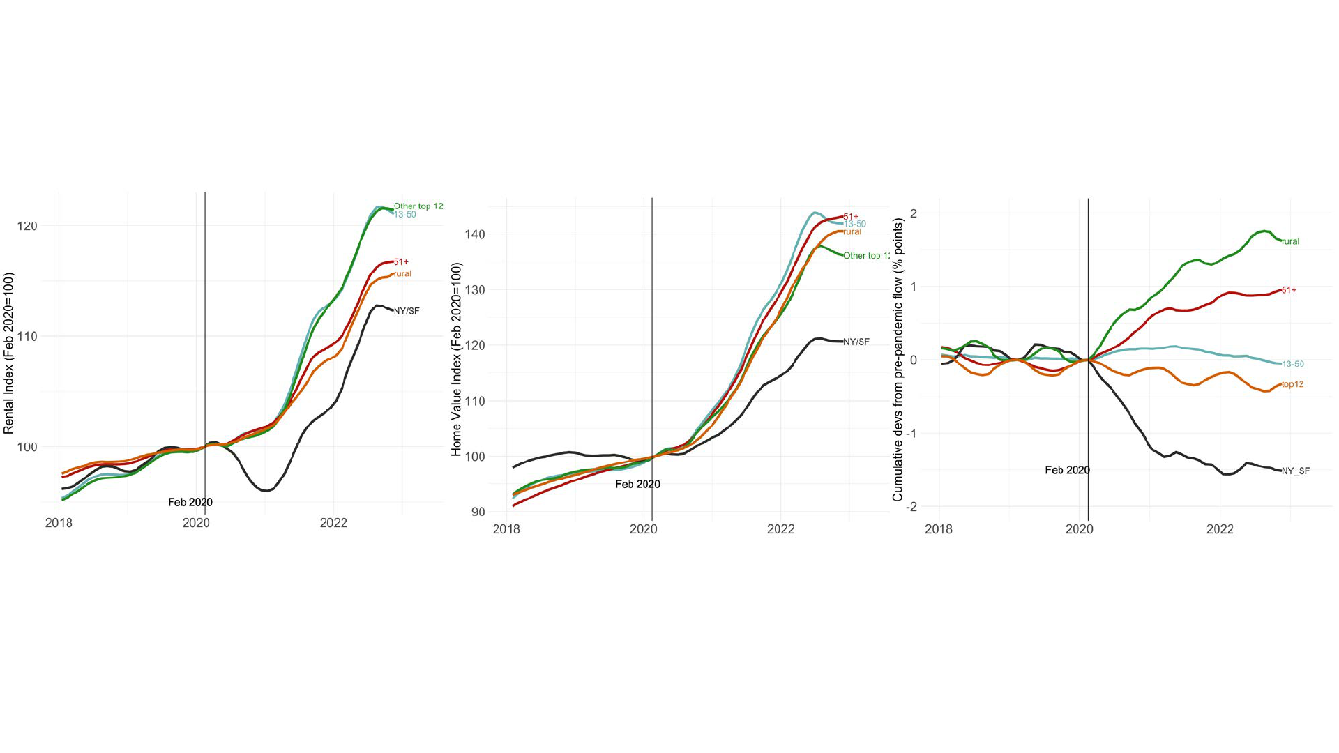
Figure 8: The largest metros, namely New York and SF, were the most affected
Notes: The panels show a population-weighted average of (a) Zillow’s rental index (b) Zillow’s home value index and (c) USPS change-of-address net inflows as a percent
of 2019 population across four buckets of metro areas. We multiply the number of household moves by the average household size from the Census Bureau, 1.7, add the
number of individual moves to calculate total population flows and then take the difference from the average flow in the year pre-pandemic. Each panel groups the data into
four buckets of MSAs by total population: NY and SF, the other top 12 MSAs, MSAs 13-50 and MSAs 51-365. Data is originally at the zip-code level before aggregation. The
population sizes of the different buckets are: top 12 metros=94.5m, metros 13-365=176m, rural=57m. Sources: USPS, Zillow, Census Bureau. Data: Jan 2018 – Nov 2022.
(a) Rents
(b) Housing prices (c) Population net inflows

Notes: The table shows the distribution of household moves post-pandemic (March 2020-Dec 2021) originating from central business districts (CBDs) and high density zip
codes (top 10% of distribution). We control for the pre-Covid trend by subtracting the distribution of moves from the period of same duration prior to Covid (May 2018 - Feb
2020). We only consider moves originating in the top 12 metros by population. We classify a household as a mover if the most recent pre-pandemic household address
(before March 2020) is different rom the most recent post-pandemic household address (during or after after March 2020). The population sizes of the different buckets are:
top 12 metros=94.5m, metros 13-365=176m, rural=57m. Sources: US Postal Service, Data Axle, US Census Bureau.
Figure 8: Over half of donut movers stayed within the same metro area
13%
High density
34%
Mid density
11%
Low density
Suburbs/exurbs of same metro
Other top 12
metros
Metros 13-365 Rural areas
58% 9% 29% 4%
0% 10% 20% 30% 40% 50% 60% 70% 80% 90% 100%
Share of additional
outflows from city
center

Table 1: Density, distance from CBD and working from home explain the donut effect.
Notes: The table shows a set of population weighted regressions of the year over year percent change in Zillow’s rental index or home value index from Feb 2020 to Feb
2022 regressed on population density, distance to CBD, and the share of residents who can WFH in 2019. Population estimates are the from the 2015-19 5-yr ACS. WFH
shares are calculated by merging the industry distribution of residents from LODES and the share of jobs that can be done from home from Dingel and Neiman (2020) at
the 2-digit NAICS level. We control for the percent change in the index over the previous 12 months (Feb 2019 to Feb 2020) due to limited historical data. We limit our
dataset to the top 12 US metros by population. All regressions include MSA fixed effects and robust standard errors. *p<.1, **p<.05, ***p<.01. Sources: Zillow, Census
Bureau, Dingel and Neiman (2020).
Percent change in index Feb 2020 – Feb 2022
Rents (1) – (4) Home values (5) – (8)
(1) (2) (3) (4) (5) (6) (7) (8)
Density
-3.049
***
-1.605
***
-2.561
***
-0.655
***
(0.238) (0.111) (0.156) (0.106)
Dist
to city center 3.455
*
2.123
***
4.718
***
3.787
***
(2.033) (0.681) (1.399) (0.162)
Share of 2019 residents that can WFH
-10.318
***
-5.501
***
-15.219
***
-9.910
***
(0.306) (0.781) (0.130) (0.865)
Observations
1,031 1,031 1,031 1,031 3,583 3,583 3,583 3,583
R
2
0.769 0.779 0.729 0.788 0.656 0.707 0.580 0.719

Notes: The table shows a set of population-weighted regressions where the dependent variables are cumulative net inflows from Feb 2020 to Feb 2022 as a percent of stock
of either population or businesses. The population stock is taken from the 2015-2019 5-yr ACS and establishment stock from the 2018 Zipcode Business Patterns. We
regress on population density, distance to city center, and the share of residents who can WFH in 2019. Population estimates are the from the 2015-19 5-yr ACS. WFH
shares are calculated by merging the industry distribution of residents from LODES and the share of jobs that can be done from home from Dingel and Neiman (2020) at the
2-digit NAICS level. We also control for the percent change in the index over the previous 12 months (Feb 2019 to Feb 2020) due to limited historical data. We limit our
dataset to the top 12 US metros by population. All regressions include MSA fixed effects and robust standard errors. *p<.1, **p<.05, ***p<.01. Sources: Zillow, Census
Bureau, Dingel and Neiman (2020).
Table 2: Density, distance from CBD and working from home explain the donut effect.
Cumulative change in variable Feb 2020 – Feb 2022 as a percent of stock
Population (1) – (4) Business establishments (5) – (8)
(1) (2) (3) (4) (5) (6) (7) (8)
Density -1.669
***
-1.144
***
-2.892
***
-0.861
***
(0.361) (0.173) (0.269) (0.174)
Dist to city center 2.305
*
0.998 4.047
**
3.353
***
(1.350) (3.082) (1.909) (0.213)
Share of 2019 residents that can WFH -6.979
***
-4.805 -12.757
***
-0.096
(0.412) (3.051) (0.279) (1.252)
Observations 3,622 3,622 3,622 3,622 3,622 3,622 3,622 3,622
R
2
0.696 0.686 0.606 0.719 0.316 0.362 0.243 0.367

Appendix A1: Donut effect is largest in top 12 cities for rents
Notes: The figure shows Zillow’s rental index grouped by population density. Panel A pools the top 12 metros by population, panel B contains metros 13-50. and panel C
gives the remaining metros (we have data on 365 in total). Zipcodes are grouped by population density or presence in a CBD. A population weighted average is taken
across all zipcodes in each bucket, and each aggregated index is normalized such that Feb 2020 = 100. Density groups are given by high = top 10%, suburb = 50-90
th
percentile, exurb = 0-50
th
percentile and populations are taken from the 2015-19 5-yr ACS. The city center is defined by taking all zipcodes with centroids contained within a
2 km radius of Central Business District coordinates taken from Holian (2019). Sources: Zillow, Census Bureau, Holian (2019). Data: Jan 2018 – Nov 2022.
(a) Top 12 MSAs (b) MSAs 13-50 (c) MSAs 51-100

Appendix A2: Net population inflows predict real estate rent and price growth
Notes: Both charts show a binscatter of the percent change in Zillow’s rental index (a) or home value index (b) from Feb 2020 to Nov 2022 on the cumulative net population
inflow as a percent of the 2015-2019 5-yr ACS population estimates at the zipcode level. We limit our dataset to the top 12 US metros by population. We control for
population density (log), the pre-trend percent change in index from Jul 2017 to Feb 2020, and MSA-fixed effects. *p<.1, **p<.05, ***p<.01. Sources: USPS, Zillow, Census
Bureau.
(a) Rental rates (b) Home values

Appendix A3: The donut effect for the largest twelve US cities: equal weighting of all zipcodes
Notes: The figure shows Zillow’s observed rental index (left) and home value index (right) in the twelve largest US metro areas. Zipcodes are grouped by population density
or presence in a CBD. Zipcode level series are first normalized to Feb 2020 = 100 and then a population-weighted average is taken across all zipcodes within a group
(reversing the order of our standard approach such as in Figure 1). Groups are given by high = top 10%, suburb = 50-90
th
percentile, exurb = 0-50
th
percentile. The city
center is defined by taking all zipcodes with centroids contained within a 2 km radius of Central Business District coordinates taken from Holian (2019). Populations are
given by 2015-19 5-yr ACS. Sources: Zillow, Census Bureau, Holian (2019). Data: Jan 2018 – Nov 2022.
(a) Rental rates (b) Home values
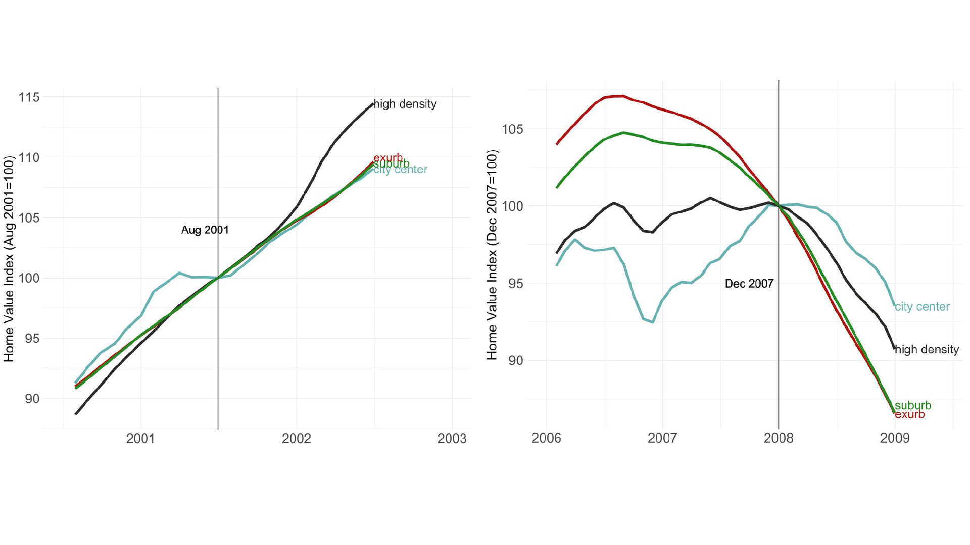
Appendix A4: Past macro shocks did not cause persistent donut effects
Notes: Both panels shows Zillow’s smoothed home value index in the twelve largest US metro areas (the smoothed index was used because the raw index is not available
before 2014). Zip codes are grouped by population density or presence in a CBD and a population-weighted average is taken across all zip codes within a group (using the
2010 Census population). Groups are given by high = top 10%, suburb = 50-90
th
percentile, exurb = 0-50
th
percentile. Panel (a) is normalized such that Aug 2001 = 100 and
panel (b) such that Dec 2007 = 100 to correspond to the 9/11 and Great Recession shocks respectively. The city center is defined by taking all zipcodes with centroids
contained within a 2 km radius of Central Business District coordinates taken from Holian (2019). Sources: Zillow, Census Bureau, Holian (2019). Data: (a) Jul 2000 – Jul
2002 (b) Jan 2006 – Jan 2009.
(a) 9/11 (b) Financial crisis of ‘08

Notes: The left panel shows cumulative net population inflows divided by 2019 population from the 2015-19 5-yr ACS. We multiply the number of household moves by the
average household size of movers from Data Axle, 1.7 and add the number of individual moves to calculate total population flows. The right panel shows the cumulative net
establishment inflows divided by the 2018 establishment stock given by the 2018 Zipcode Business Patterns. Both series are cumulated starting from Jan 2018 after
differencing monthly inflows from the average flow in the year pre-pandemic. This shows the cumulative flows above their pre-pandemic trend over this period. Zipcodes
are grouped by population density or presence in a CBD. A population weighted average is taken across all zipcodes in each bucket. Groups are given by high density =
top 10%, suburb = 50-90
th
percentile, exurb = 0-50
th
percentile. The city center is defined by taking all zipcodes with centroids contained within a 2 km radius of Central
Business District coordinates taken from Holian (2019). Sources: USPS, Census Bureau, Holian (2019). Data: Jan 2018 – Nov 2022.
Appendix A5: Cumulative flows versus the pre-pandemic trend follow the donut effect with
sharp outflows from CBDs
(a) Cumulative net population inflows as a percent of total
(b) Cumulative net establishment inflows as a percent of total

Notes: Both panels display heat maps of the cumulative net inflows (moves in – moves out) from Feb 2020 to Nov 2022 as a percent of population (2015-19 5-yr ACS) at
the zipcode level. The left panel shows the Boston-Cambridge-Newton, MA-NH MSA and the right panel shows Los Angeles-Long Beach-Anaheim, CA. Data on flows are
calculated using USPS National change of address dataset. We multiply the number of household moves by the average household size from the Census Bureau, 2.5, and
add the number of individual moves to calculate total population flows. Sources: USPS, Census Bureau.
Appendix A6: Change of address flows occur from the city center to the suburbs
CBD
CBD
Boston, MA Los Angeles, CA

Notes: This chart shows a county level scatterplot and regression of official migration vs change-of-address flows. The y-axis is the county-level net domestic in-migration
from 2017-19 taken from the US Census Bureau. The x-axis is the net population inflow as measured by USPS change-of-address data. We multiply the number of
household moves by the average household size from the Census Bureau, 2.5, and add the number of individual moves to calculate total population flows. Note that USPS
data do not include inflows from other countries. Sources: USPS, Census Bureau.
Appendix A7a: USPS Change of address flows follow official Census migration statistics
(a) Flows – censored at 1/99%
(b) Flows as %of pop – censored at 1/99%
Y=1.7e3+0.29*X, R^2=0.30 Y=0.005+0.28*X, R^2=0.26

Appendix A7b: Data Axle levels match ACS levels for population and income
(a) Population levels (b) Median household income
Notes: This chart shows a county level scatterplot and regression of official population and income data from the 2015-19 pooled American Community Survey (ACS) vs
linked population and income data constructed from Data Axle address files. The y-axis is the (a) county-level population or (b) median household income taken from ACS
data. The x-axis is the (a) county-level population or (b) median household income from Data Axle’s household-address files. Sources: Data Axle, American Community
Survey, Census Bureau.
Y=3.00e2+.62*X, R^2=0.90 Y=2.9e4+0.76*X, R^2=0.71

Notes: This chart shows a county level scatterplot and regression of official migration vs change-of-address flows. The y-axis is the county-level net domestic in-migration
from 2017-19 taken from the US Census Bureau. The x-axis is the net population inflow as measured by linked address level files provided by Data Axle. We calculate
population flows by summing the head of household, spouse and children for each household. Sources: USPS, Census Bureau, Data Axle.
Appendix A7c: Data Axle flows follow official migration statistics
(a) Net inflow– censored at 1/99%
(b) Flows as %of pop – censored at 1/99%
Y=5.28e2+0.93*X, R^2=0.49 Y=2.36e-5+1.26*X, R^2=0.63

Notes: This chart shows a county level scatterplot and regression of public USPS change-of-address flows vs flows derived from Data Axles quarterly address files. The y-
axis is the county-level change of address flows from the publicly available USPS files. The x-axis is the net population inflow as measured by linked address level files
provided by Data Axle. We calculate population flows by summing the head of household, spouse and children for each household. Sources: USPS, Census Bureau, Data
Axle.
Appendix A7d: Data Axle flows follow public USPS flows
(a) Flows – censored at 1/99%
(b) Flows as %of pop – censored at 1/99%
Y=792+1.19*X, R^2=0.52 Y=-0.02+1.59*X, R^2=0.32
